


Abstract
This paper proposes an approach to the specification and model checking of a large, important class of distributed algorithms called control algorithms (CAs), which are superimposed on underlying distributed systems (UDSs). The approach is based on rewriting logic by moving from its object level to the meta-level. We introduce the idea of specifying CAs as meta-programs that take the specifications of UDSs and automatically generate the specifications of the UDSs on which the CAs are superimposed (UDS-CAs). Due to many options, such as network topologies, even fixing the number of each kind of entities, such as mobile support stations (MSSs) and mobile hosts (MHs) in a mobile checkpointing algorithm, there are many instances of a UDS. To address the problem, we generate all possible initial states of a UDS for a fixed number of each kind of entities such that some constraints, such as MSSs strongly connected with a wired network, are fulfilled and conduct model checking for each of the initial states. We demonstrate the usefulness by reporting on a case study where a counterexample is found for some specific initial states but not for the other initial states, detecting a subtle flaw lurking in a mobile checkpointing algorithm.
1 Introduction
Key software systems on which humans rely are in the form of distributed systems. Due to the distributed aspects, they have raised many serious problems that require global solutions. It is necessary to use many essential distributed algorithms, such as termination detection algorithms, snapshot recording algorithms and checkpointing algorithms. A key feature of these algorithms is that their executions are superimposed on the underlying application executions. Such distributed algorithms are called control algorithms (CAs) [16]. Based on our surveys of [16] and [32], there are |$\sim $|30% problems addressed by CAs. These problems require monitoring application executions or performing various auxiliary functions, such as creating a spanning tree, creating a connected dominating set, achieving consensus among the nodes, distributed deadlock detection, global predicate detection, termination detection, global state recording and checkpointing. CAs are therefore a large and important class of distributed algorithms.
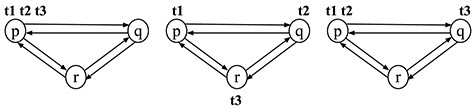
Distributed systems are quite complex and therefore difficult to design, build and verify. It is challenging to ensure the correctness of a distributed system for two main reasons: distribution and asynchrony. It may not be until computation that the errors are noticed to be present. Model checking [2] is a popular automatic formal technique and is highly suitable for formally verifying such systems. CAs have raised a challenge for verification by model checking, since such algorithms cannot be specified independently of the underlying systems. Although some CAs have been specified and model checked in [4, 5, 31], the underlying systems on which CAs are superimposed must all be specified directly by humans (Fig. 1a). If the same CA is to be verified for different underlying distributed systems (UDSs), we need to write new specifications of UDS on which the algorithm is superimposed (UDS-CA). This consumes time and exhausts the specifiers due to repetition.
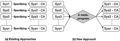
The existing approaches and our new approach to specifying CAs; |${Sys1, \dots , Sys}n$| are UDSs and |${Sys1\mbox{-}CA, \dots , Sys}$| n |${\mbox{-}CA}$| are the UDSs on which a CA is superimposed.
We can therefore propose a new approach so that we only need to specify a CA once. However, it is challenging to specify CAs in almost all existing specification languages for model checkers, such as PROMELA [14], because it is necessary to treat a UDS as data handled by CAs. Moreover, two different systems (a UDS and the UDS-CA) may need to be considered to model check some properties for CAs, while almost all existing model checkers (to our knowledge), such as SPIN [14] and NuSMV [7], do not support this.
Our solution. We have investigated one possible solution that is to apply meta-programming techniques to the above-mentioned challenges. We propose an approach that aims to avoid repetition by specifying a CA as a meta-program that takes the specification of a UDS and generates the specification of the UDS-CA. This is depicted in Fig. 1b. The model checking is conducted at the meta-level as well. The meta-level makes it possible to model check the properties whose formalizations involve both a UDS and the UDS-CA. Distributed snapshot reachability (DSR) property is one of such properties (see Section 6).
It is necessary to provide an initial state of a UDS to model check that the UDS-CA enjoys a desired property. A major challenge is that counterexamples can be found for some initial states, while they cannot be found for others. Even fixing the number of every kind of entities, such as mobile support stations (MSSs) and mobile hosts (MHs) in a mobile checkpointing algorithm, used in a UDS, there may be more than one UDS due to many options, such as network topologies. To address the problem, we generate all possible initial states of a UDS for a fixed number of each kind of entities. However, since too many initial states could be generated, however, we use some constraints to keep the number moderate. One possible constraint is that MSSs are strongly connected to the wired network. We demonstrate the usefulness by reporting on a case study (presented in Section 7) where a counterexample is found for some particular initial states but not for the other initial states, detecting a subtle flaw lurking in a mobile checkpointing algorithm.
The Chandy–Lamport distributed snapshot algorithm (CLDSA) has been considered in some of our research papers [11–13]. In [13], we propose a method that formalizes a UDS and the UDS-CLDSA as state machines, in which the formalization of a UDS-CLDSA is generated from that of the UDS precisely. The paper [13] is then extended and revised in [12], where we give a more faithful formal definition of the DSR property and prove that CLDSA does not alter the behavior of a UDS. This paper is a revised and extended version of the paper [11] published at ICDCS 2017, which reported the case study of CLDSA. However, in [11], we only consider CLDSA, while in this paper we make the approach generic so that it can be applied to a class of CAs, such as a checkpointing algorithm.
Related work. Because it is complex, error-prone and hard to design distributed systems, many researches on formal specification and verification of such systems have been conducted [1, 5, 15, 33]. Several studies are motivated by verification of snapshot algorithms. Among them, [5] and [14] consider CLDSA. In [14], CLDSA is modeled in PROMELA, and then the model is simplified to be verifiable. However, only the UDS superimposed by CLDSA is modeled. The authors in [5] focus on developing snapshot algorithm with a formal proof that guarantees its correctness by using the Event-B framework and refinement. Not only two, but many state machines are modeled to derive the algorithms by many refinement steps. Their experiments are conducted on fixed networks.
Meta-programming technique is powerful in the processing of other programs, which are treated as data. In [29], the authors developed a meta-program for debugging normal logic programs. In [10], a meta-interface mechanism (called a quality connector) for reducing the life-cycle costs of distributed real-time and embedded systems is proposed. Although many researches have been conducted on application of meta-programming technique, as far as we know, the research on applying meta-programming to specifications of distributed algorithms has not been conducted so far.
Maude has been used to formally analyze various kinds of distributed systems/protocols. We mention some recent studies on the formal analysis of such systems with Maude.
Data are partially replicated in different servers in distributed transaction systems (DTSs) to make such systems scalable and fault tolerant. DTSs need to guarantee various consistency properties from weak ones such as read atomicity through various forms of snapshot isolation to stronger serializability properties. Liu et al. [21] propose a way to formally specify DTSs and nine consistency properties in Maude and a way to formally verify that DTSs enjoy those consistency properties with Maude. They have built a tool that automates the formal verification in Maude. One core idea is to formalize/implement the transformation from a Maude specification of a DTS into one with a monitor as a meta-level function monitorRules: Module -> Module in Maude. They have conducted case studies in which several DTSs are formally analyzed. Among the DTSs formally analyzed with their technique are ROLA [19], Walter [20] and RAMP [18].
It is really challenging to develop good cloud computing systems. This is because such systems are distributed ones and need to meet high performance requirements, such as high availability and throughput, and low latency, even with network congestion and faults. Meseguer [27] addresses how to use formal methods, especially Maude and its related techniques, to achieve high-quality cloud computing systems based on some studies on the formal analysis of distributed systems conducted by him together with his colleagues. Meseguer enumerates some challenges: (i) the formal methods used have to naturally support distributed design and analysis, (ii) the formal notations need to be easily understood by engineers, (iii) correctness properties should be able to be formally analyzed and (iv) formal analysis results should be able to answer performance questions as well as correctness questions. Furthermore, all this should be conducted before actually implementing such systems, which can be done with Maude. One possible limitation is that systems described in Maude cannot be used as real systems that can be deployed. Since Maude supports TCP/IP sockets as built-in objects, however, systems described in Maude can be easily distributed. Close to our method, Meseguer [26] proposes formal patterns for distributed systems. He tries to give a generic and reusable pattern to design and specify distributed algorithms. Rewriting logic at the meta-level is also one of the main theories used to describe these formal patterns.
It is necessary to assume that there are intruders who act as ordinary participants (principals) as well so as to analyze security protocols. It is know that if there is an attack to a security protocol by using multiple Dolev–Yao intruders, the attack can be carried out by using a single Dolev–Yao intruder. Thus, a single Dolev–Yao intruder is often used for the security protocol analysis. It is also know that it is not appropriate to use a single Dolev–Yao untruer so as to analyze cyber-physical security protocols (CPSPs) because Dolev–Yao intruders do not have any physical properties. To address this issue, timed Dolev–Yao intruder model is proposed [3]. There is, however, a question: how many intruders are enough for verification and where should they be placed? Nigam et al. [28] answer the question and their answer is as follows: it is enough to consider one intruder per protocol participant, thus bounding the number of timed intruders. They also build a tool supporting the formal analysis of CPSPs in Maude.
Although many studies on the formal analysis of distributed systems/protocols with Maude have been conducted and many formal tools have been developed by using the meta-programming functionalities of Maude, to the best of our knowledge, no studies on the formal analysis of distributed algorithms/protocols as meta-programs have been done. Therefore, we can claim that our proposed technique to formally specify CAs as meta-programs in Maude.
Our contribution. (1) Specification: we introduce an idea of specifying a CA as a meta-program that allows the algorithm to be specified once. Our approach reduces time and effort by eliminating the need to repeat the specification.
(2) Model checking: we propose a technique that takes the number of each kind of entities used, generates all possible initial states and conducts model checking experiments for all initial states making it more likely to detect a subtle flaw lurking in a CA. Our model checking found two subtle errors in a checkpointing algorithm. Properties involving a UDS and the UDS-CA can also be addressed using the proposed technique.
The outline of the paper. Section 2 introduces CAs. Section 3 introduces Maude and meta-programming in Maude. The new approach is introduced in Sections 4 and 5. Two algorithms, namely snapshot and checkpointing algorithms, are taken as case studies, which are described in Sections 6 and 7. Section 8 finally concludes the paper.
For the experiments reported in this paper, a computer with a 2.9 GHz processor Intel Xeon E5-4655 and 256 GB RAM was used.
2 Control Algorithms
A distributed system consists of independent entities that are connected and communicate by passing messages through communication networks. The essential characteristic of CAs is that they are superimposed on UDSs and do not interfere with them (Fig. 2) [16, 32]. In other words, they run concurrently with, but do not alter the behavior of UDSs.
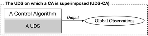
A CA’s execution is superimposed on the underlying application executions.
Let us consider the following simple, but non-trivial, CA as an example. The algorithm is called ‘four-counter algorithm (FCA)’ [24, 32] for termination detection in an asynchronous atomic model.
Computation model. Let |$p_1, \ldots , p_n$| be |$n$| processes fully connected by network. Each |$p_i$| has a local variable denoted |$mode_i$| whose value is either |$\textrm{active}$| or |$\textrm{passive}$|. Initially, some processes, at least one, are in the |$\textrm{active}$| mode. When |$p_i$| is active, it can perform local computations and send messages to the other processes. When a message reaches |$p_j$|, |$p_j$| sets |$mode_j$| to |$\textrm{active}$|. Messages are delivered reliably and without error in finite but arbitrary time and may or may not be in the order sent. The atomic model assumes that it only takes time to deliver a message, but the destination process does anything immediately upon receiving the message, such as updating its internal state.
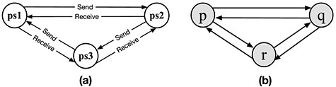
Figure 3 describes a UDS consisting of three processes |$\textrm{p}, \textrm{q}, \textrm{r}$| and two tokens |$\textrm{t}_1$|, |$\textrm{t}_2$|. The state of a process depends mainly on the set of tokens it has. Each process has two actions: (i) consume one of its tokens or send the token to another process by putting the token into one of its outgoing channels if the process is |$\textrm{active}$| and (ii) receive a token from one of its incoming channels and become |$\textrm{active}$| if it is |$\textrm{passive}$|. If a process has no tokens, it can become |$\textrm{passive}$| and then remains |$\textrm{passive}$| until it receives a token. Initially, only |$\textrm{p}$| is active, |$\textrm{t}_1$| belongs to |$\textrm{p}$| and |$\textrm{t}_2$| belongs to |$\textrm{q}$|.
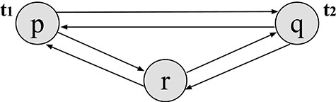
An initial state of the 3-processes, 6-channels and 2-tokens system.
Termination detection problem. Let |$c[i,j]$| denote the channel from |$p_i$| to |$p_j$| and |$\textrm{empChan}$| denote the empty channel. A distributed computation is said to be terminated if and only if (iff): for all |$i$|, |$mode_i$| = |$\textrm{passive}$| and for all |$i,j$|, if there exists |$c[i,j]$|, then |$c[i,j]$| = |$\textrm{empChan}$|.
The FCA. The idea underlying the algorithm is simple: it detects termination by counting and comparing the numbers of messages that have been sent and received. It claims termination when the total number of messages sent equals the total number of messages received.
Let us consider a simple version of the algorithm based on an inquiry-based principle. Each |$p_i$| is required to count the number |$sent_i$| of messages it has sent and the number |$rec_i$| of messages it has received. It is assume that there is an observer in charge of the termination detection. To start, the observer requests each |$p_i$| to send it the pair (|$sent_i$|,|$rec_i$|). When the observer has all the pairs, it computes the total numbers |$S$| and |$R$| of the messages sent and received. If |$S$| = |$R$|, it claims that the system has terminated. Otherwise, it starts its next inquiry.
3 Maude and Meta-programming in Maude
3.1 Maude
Maude [8] is a specification/programming language based on rewriting logic, with a powerful system (or environment). Rewriting logic allows to specify distributed systems in a natural way [25], and the Maude system has a linear temporal logic (LTL) model checker [8, 23]. Therefore, Maude allows model checking whether a distributed system specified in Maude enjoys properties expressed in LTL.
The basic units of specifications/programs are modules. A module contains syntax declarations and thus provides a suitable language for describing a system. A module consists of the sort, sub-sort, operator, variable, equation and membership declarations, as well as rewrite rule (or rule) declarations. A sort denotes a set, corresponding to a type in conventional programming languages. For example, the sort Nat denotes the set of natural numbers. Between sorts there is a relation identical to the subset relation. A sort is a subsort of another sort iff the set denoted by the former is a subset of the set denoted by the latter, and the latter is called a supersort of the former. Let Zero and NzNat be the sorts denoting |$\{0\}$| and the set of non-zero natural numbers, both of which are subsets of the set of natural numbers. Zero and NzNat are subsorts of Nat and Nat is a supersort of Zero and NzNat.
A distributed system can be formalized as a state machine. A state machine consists of a set of states, some of which are initial states, and a binary relation over the states.
A state machine |$M \triangleq \langle S, I, T \rangle $| consists of
a set of states |$S$|;
a set of initial states |$I \subseteq S$|;
a total binary relation over states |$T \subseteq S \times S$|.
A state machine is specified in Maude as a system module, which consists of three parts:
Syntax part, which defines all notations describing the system, in which sorts and operators are declared;
Initial part, which defines the initial states of the system; and
Transition part, which defines the behavior of the system.
The following part shows how to formalize and specify a UDS. Let us consider the system shown in Fig. 3 as an example.
The syntax part. Let Pid, Mode and Token be the sorts for process identifiers, process modes and tokens; p, q and r be the constants of Pid; active and passive be the constants of Mode; and t1 and t2 be the constants of Token. Let TknSet be the sort for token soups. Local states of processes and channels are expressed as so-called observable components, which are |$name$|-|$value$| pairs. Let OCom be the sort for observable components. The local state of each process whose identification is |$p$| is expressed as an observable component <|$p$| : |$md$|,|$ts$|>, where |$p$| is the name and ‘|$md$|,|$ts$|’ is the value, a pair of a process mode and a token soup. Let Msg be the sort for messages and the supersort of Token. So, tokens are messages. Let Chan be the sort for message soups. The local state of each channel from |$p$| to |$q$| is expressed as the observable component [|$p$|,|$q$|: |$ms$|], where ‘|$p$|,|$q$|’ is the name and |$ms$| is the value, which is a message soup.
Global states of the system are expressed as soups of observable components for which Config is used as the sort. A sort and the set denoted by the sort are used interchangeably in this paper. We often use associative–commutative collections as key data structures. Such collections are referred as soups. Suppose that if |$Soup$| is the sort for a soup, the constant emp|$Soup$| denotes an empty soup.
An operator is declared as follows:
|$f: S_1 \ldots S_n \rightarrow S$|,
where |$S_1, \dots , S_n, S$| are sorts and |$n \geq 0$|. Note that -> may be used instead of |$\rightarrow $|. |$S_1 \ldots S_n$|, |$S$| and |$S_1 \ldots S_n \rightarrow S$| are called the arity, sort and rank of |$f$|, respectively. When |$n = 0$|, |$f$| is called a constant. |$f$| takes a sequence of |$n$| terms of |$S_1, \dots , S_n$| and makes a term of |$S$|, which we will describe in a moment. Operators denote functions or data constructors. Each variable has its own sort.
The syntax part of the module is as follows:

where the keywords sort, subsort and op are used to declare a sort, a subsort relation and an operator, while sorts, subsorts and ops can be used for multiple such things. An operator without any arguments is called a constant, such as t1 and t2. The keyword ctor indicates that the operators are constructors, and the keywords assoc and comm indicate that the binary operators are associative and commutative, respectively. id: empTknSet indicates that the operator empTknSet is the identity element. An underscore _ is a place holder where an argument is put.
Terms of a sort |$S$| are inductively defined as follows: (i) every variable whose sort is |$S$| is a term of |$S$| and (ii) for each operator |$f$| whose rank is |$S_1 \ldots S_n \rightarrow S$| and |$n$| terms |$t_1, \ldots , t_n$| of |$S_1 \ldots S_n$|, |$f(t_1, \ldots , t_n)$| is a term of |$S$|. If |$S$| is a subsort of |$S^{\prime}$| and |$t$| is a term of |$S$|, |$t$| is also a term of |$S^{\prime}$| but not vice versa. Note that if |$n = 0$|, then |$f$| is a term of |$S$|. An operator may contain underscores, e.g. op [_, _, _]: Pid Pid Chan -> OCom. When this is the case, a notation other than |$f(t_1, \ldots , t_n)$| is used. For example, [p, r: empChan] is a term of the sort OCom, where p and q are terms of the sort Pid and empChan is a term of the sort Chan, representing that the channel from p to q is empty. By using operators containing underscores, we can define context-free grammars.
States of the system are expressed as terms of the sort Config. For example, (¡P: active, TS¿) ([P, Q: empChan]) BC expresses any state such that the process P has the status active and the channel from P to Q is empty. Such a state may have some more processes and some channels that are expressed as BC. An equation declares that two terms are equal. Ground constructor terms are those composed of constructors only. Ground constructor terms of the sort Config express concrete states of the system.
The initial part. The initial state is expressed as a ground constructor term of the sort Config. Terms representing states are called configurations. States and configurations may be used interchangeably in this paper. In this system, there is one initial configurations in which |$p$| is active and has |$t_1$|, |$p$| is passive and has |$t_2$|, |$r$| is passive and has no token and all channels have no token.

where init equals the term expressing the initial configurations.
The transition part. Actions performed by processes are formalized as state transitions, which are specified as rules. One rule is as follows:

where P, Q, T, TS, CS and BC are variables of Pid, Pid, Token, TknSet, Chan and Config, respectively. sndToken is the label given to the rule. The rule states that if P owns T and has an outgoing channel to Q, then P can put T into the channel. By substituting P, Q, T, TS, CS and BC with p, q, t1, empTknSet, empChan and the following term:

respectively, the left-hand side of the rule sndToken is the same as the term init and can then be applied to the term. If so, the term changes to the following:

In this way, state transitions are specified as rules.
Although, each action is described by a transition rule, there may be more ground instances of the transition rules. This is due to the number of states for each process, the number of channels, the number of states for each channel, etc. Given a transition rule L |$\Rightarrow $| R, one obtains a ground instance of the transition rule by replacing each variable in L |$\Rightarrow $| R with a ground constructor term (or value) of the sort of the variable.
Let |$TR_{UDS}$| be the set of all ground instances of all transition rules.
A UDS is formalized as state machine |${M}_{UDS}$| |$\triangleq \langle $||${S}_{UDS}$|, |${I}_{UDS}$|, |${T}_{UDS}$||$\rangle $|. |$S_{UDS}$| is the set of all ground constructor terms whose sorts are Config. |$I_{UDS}$| is a subset of |$S_{UDS}$| such that for each state |$s$| |$\in $| |$I_{UDS}$|, for each channel |$c$| in |$s$|, the message queue in |$c$| is empty. |${T}_{UDS}$| is the binary relation over |${S}_{UDS}$| made from |${TR}_{UDS}$|.
The state machine formalizing a UDS is |${M}_{UDS}$| |$\triangleq $| |$\langle $||${S}_{UDS}$|, |${I}_{UDS}$|, |${T}_{UDS}$||$\rangle $|, where
|$S_{UDS}$| is the set of all ground constructor terms whose sorts are Config;
|$I_{UDS}$| is a subset of |$S_{UDS}$| such that (|$\forall s \in $| |${I}_{UDS}$|)(|$\forall c \in $| chans(|$s$|)) (msg(|$c$|) = empChan);
|$T_{UDS}$| is the binary relation over |$S_{UDS}$| defined as follows: {(|$C$|, |$C^{\prime}$|) |$\mid $| |$C$|, |$C^{\prime}$| |$\in $| Config, |$L$| |$\Rightarrow $| |$R$| |$\in $| |$TR_{UDS}$|, |$\exists $| |$C^{\prime\prime}$|.(|$C$| = |$L$| |$C^{\prime\prime}$| |$\land $| |$C^{\prime}$| = |$R$| |$C^{\prime\prime}$|)}
Function |$\textrm{chans}$| gets all channels of a state |$s$| |$\in $| |${S}_{UDS}$| and |$\textrm{msg}$| gets the state of a channel |$c$| in |$s$|.
Let SYS be the module in which the system is specified. We will interchangeably use ‘state transitions’ and ‘rules’ in the rest of the paper.
3.2 Meta-program in Maude
Meta-programming is a programming technique endowed with the ability to treat programs as data. A meta-program takes a program and performs some useful computation, such as analyzing the program and transforming it into another. Meta-programming is the main technique used in our rewriting logic-based method, in which important aspects of its meta-theory can be represented at the object-level in a consistent way. In Maude, meta-programming has a logical, reflective semantics because Maude is designed and implemented based on the fact that rewriting logic is a reflective logic [9]. Maude strongly supports meta-programming since all essential functionalities have been implemented in the module META-LEVEL.
Terms are only data structures available in Maude and programs/specifications are composed of modules. It is necessary and sufficient to be able to build modules as terms in meta-programs. We need to represent their components, such as operator and rule declarations, as terms. Terms representing modules, operator declarations, rule declarations, etc. are called their meta-representations. Sorts are meta-represented as data in the sort Sort, which is a subsort of the sort Qid of quoted identifiers. For example, ’Bool and ’Nat are terms of this sort. Maude terms are meta-represented as elements of the sort Term for terms. The sort Term is a supersort of the sorts Constant for constants and Variable for variables, which are subsorts of the sort Qid. Constants are quoted identifiers that contain the constant’s name and its type separated by a ‘.’, e.g. ’true.Bool. Similarly, variables contain the variable’s name and its type separated by a ‘:’, e.g. ’X:Bool.
Arguments of an operator are expressed as a list of terms for which the sort TermList that is a supersort of the sort Term is prepared. A list of terms is built with the constructor _,_. For example, the term ¡ P: active, t1 ¿ is meta-represented as the following term of the sort TermList:

where ‘¡_‘:_‘,_‘¿ is the meta-representations of the operator ¡ _: _, _ ¿ and ’P:Pid, ’actine.Mode, ’t1.Token is a list of terms and its sort is TermList. The term list is constructed by one variable ’P:Pid and two constants ’t1.Token and ’active.Mode.
Modules are meta-represented as a term of the sort Module of modules. A system module is expressed as the following operators:

where Header, ImportList, SortSet, SubsortDeclSet, OpDeclSet, MembAxSet, EquationSet and RuleSet are the sorts for the meta-representations of the name of the module, imported submodules, sort declarations, subsort declarations, operator declarations, membership declarations (that are not used in the paper), equation declarations and rule declarations, respectively.
Let us demonstrate how a meta-program modifies a specification. Suppose that we specify the natural numbers in a module NAT, where the natural numbers are defined as follows: (i) 0 is a natural number and (ii) for every natural number N, s(N) is a natural number.

Given the module NAT, a problem is to transfer it to another module called NAT+ where the operator + is added. To solve this problem, we implement a meta-program T that transfers NAT into NAT+.
Maude is equipped with rich meta-programming facilities to enable this and more. For example, Maude provides several operators that allow you to move between the object level and the meta-level. We can write a meta-program in Maude by importing the module META-LEVEL. Module META-LEVEL provides many useful and efficient built-in functions for moving between reflection levels, such as upModule, upSorts, upTerm and downTerm. The functions upModule takes as arguments the meta-representation of the name of the module |$M$| and a Boolean |$b$| and returns the meta-representation of the module |$M$|. If |$b$| is true, the meta-representations of the module imported by |$M$| are also generated. We can get the meta-representation of the module NAT as shown above by using the function upModule.

where the first argument ’NAT is the meta-representation of the name of the module NAT. Given the name H of a module, the meta-representation of the name is ’H, whose sort is Header. We can use the function upTerm to obtain the meta-representation of a term and use the function downTerm to recover the term. |$\textbf{NAT}$| is represented at the meta-level as a term |$\textbf{t}$| as follows:

where the second line starting with sort is for sort declarations. The two lines starting with op are for operator declarations. Since the module NAT has no membership axioms, no equations and no rules, those fields are filled, respectively, the constant none of the sort MembAxSet, none of the sort EquationSet and none of the sort RuleSet.
A meta-program can be implemented as a function that has Module as one of its arguments. The meta-program T takes the term t as an input, modifies it and returns a term t’, which is the meta-representation of NAT+, which defines operator +. To this end, we define T with two sub-functions reName and addOpe that rename the name of a module and add a new operator declaration to the module.

where … are some variable and equation declarations. These function take a meta-representation of a module and modify it. For instant, the sub-function addOpe is defined as follows:

where H, IL, etc. are variables of the corresponding sorts.
Let getSort be the function that gets the sort of a module defining numbers, e.g. getSort(upModule(’NAT, false)) = ’Nat.

The declaration of the operation + is as follows:

Finally, the function T is implemented.

The function T takes the meta-presentation of the module NAT as an input T(upModule(’NAT, false)) and then returns a term t’ as follows:

The term t’ is the meta-representation of the following module, which can be obtained by using the function downModule to recover from the above meta-representation of the module.

where the name of the module is renamed and the declaration of the operation + is declared.
Suppose that we specify the integer numbers in a module INT, where the integer numbers are defined as follows: (i) zero is integer number, (ii) for every an integer I, p(I) is an integer number and (iii) for any integer I, -(I) is an integer number.

If we want to change the name of the module INT to INT+ and add the declaration of the operation + to the module, the function T can be used: T(upModule(’INT, false)). We then get the modified module INT+.

The meta-program T is used to modify different modules, e.g. NAT and INT. Although the above example is simple, it introduces our idea to specify a CA as a meta-program in Maude.
For the meta-representation of a module in which a state machine is specified, Maude provides the ability to search its reachable states for states so that some requirements are satisfied, which is done by the operator metaSearch.
4 Specifying a CA as a meta-program
4.1 Meta-programs as formal specifications
A UDS-CA is viewed in two layers: the UDS as the core layer and the algorithm work as the top layer. Existing approaches repeatedly specify a CA for each different UDS. The goal is to specify a CA as it is once to avoid repetition. To this end, the CA is formalized as a transformer |$T$| that takes the state machine |$M_{ UDS} $| and returns another state machine |$M_{ UDS \mbox{-} CA }$| that formalizes the UDS-CA.
For a state machine |${M}_{UDS}$| |$\triangleq \langle $||${S}_{UDS}$|, |${I}_{UDS}$|, |${T}_{UDS}$||$\rangle $| formalizing a UDS, |$T$| is a transformer that takes |$M_{UDS}$| and returns the state machine |$M_{UDS\mbox{-}CA}$| |$\triangleq $| |$T$|(|$M_{UDS}$|) |$\triangleq $| |$\langle T_{State}$|(|${S}_{UDS}$|), |$T_{Init}$|(|${I}_{UDS}$|), |$T_{Irans}$|(|${T}_{UDS}$|)|$\rangle $| formalizing the UDS-CA.
Our fundamental idea is that the transformer is specified as a meta-program that takes a specification of a UDS and transforms it into the specification of the UDS-CA as shown in Fig. 4. The meta-program is the transformer and is implemented based on the operation of the algorithm but independent of the behavior of a UDS.

A CA is specified as a meta-program.
4.1.1 The transformer
Although the idea is generic, we use Maude meta-programming to implement the idea. The following part explains how the meta-program is constructed.
The transformer is implemented as a meta-program T, which is divided into three sub-programs T-State, T-Init and T-Trans corresponding to |$T_{\textrm{State}}$|, |$T_{\textrm{Init}}$| and |$T_{\textrm{Trans}}$|, respectively, handling the syntax part (|$S$|), the initial part (I) and the transition part (|$R$|). The meta-program T takes a module specifying a UDS as its meta-representation. Its three sub-functions then modify three corresponding parts of the specification (Fig. 5).
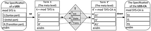
Process of transformation from UDS to UDS-CA with T, a specification of CA.
T-State. We may need to modify some of the existing notations of a UDS and/or add other new notations to describe the UDS-CA. For example, the UDS-CA may need to use control messages that are different from the computation messages used by a UDS and/or use additional components to store some information observed by the CA. T-State preserves all these observable components of the relevant UDS and may add new observable components for CA.
States of a UDS are expressed as soups (associative-commutative collections) of observable components, where observable components are name-value pairs (|$name$|: |$value$|) and name may have parameters. A state of a UDS is expressed as follows:
|$s_{UDS}$| = (|$name_1$|: |$val_1$|) … (|$name_n$|: |$val_n$|)
where |$name_i$| is a name, |$val_i$| is a value and (|$name_i$|: |$val_i$|) is an observable component.
States of a UDS-CA are also expressed as soups of observable components, but we use the terminology meta-observable components instead of observable components to distinguish states of the UDS-CA from those of the UDS. A state of the UDS-CA is expressed as follows:
|$s_{UDS\mbox{-}CA}$| = (|$base\mbox{-}state$|: (|$name_1$|: |$rev\mbox{-}val_1$|) … (|$name_n$|: |$rev\mbox{-}val_n$|)) (|$ctl\mbox{-}name_1$|: |$ctl\mbox{-}info_1$|) … (|$ctl\mbox{-}name_m$|: |$ctl\mbox{-}info_m$|)
where (|$base\mbox{-}state$|: …) and (|$ctl\mbox{-}name_j$|: |$ctl\mbox{-}info_j$|) are meta-observable components.
The meta-observable component |$base\mbox{-}state$|1 stores the state of a UDS and the meta-observable component |$ctl\mbox{-}name_j$| stores control information for the CA. The sort |$SSort_i$| of a value |$rev\mbox{-}val_i$| stored in the observable component |$name_i$| of the UDS-CA state is the same as the sort |$Sort_i$| of a value |$val_i$| stored in the same observable component of the UDS state or a super-sort of |$Sort_i$|. For each state of UDS, there can in general be several different states of UDS-CA, but for each state of UDS-CA there is one state of UDS. There is a function |$f$| that takes a state of the UDS-CA and returns a state of the UDS.
|$f$|(|$s_{UDS\mbox{-}CA}$|) = (|$name_1$|: |$f_1(rev\mbox{-}val_1)$|) … (|$name_n$|: |$f_n(rev\mbox{-}val_n))$|
where |$f_i$| is a function that takes a value of |$SSort_i$| and returns a value of |$Sort_i$|. If |$SSort_i$| is the same as |$Sort_i$|, |$f_i$| is the identity function. The function |$f$| gets rid of all the meta-observable components |$ctl\mbox{-}name_j$|.
The following requirement called the T-State requirement must be satisfied.
For each |$s_{UDS\mbox{-}CA}$| |$\in $| |$S_{UDS\mbox{-}CA}$|, |$f$|(|$s_{UDS\mbox{-}CA}$|) = |$s_{UDS}$| |$\in $| |$S_{UDS}$|
What is needed to transform the states of the UDS into the states of the UDS-CA, such as adding |$SSort_i$| and meta-observable components, is done by T-State. The T-State function takes the syntax part, modifies it and returns a new set of syntax declarations containing all notations describing the UDS-CA.
T-Init. An initial global state of the UDS-CA must contain not only the initial values of the UDS but also the initial values that depend only on the CA. Consider an initial state |$s_{UDS}$| of the UDS:
|$s_{UDS}$| = (|$name_1$|: |$val_1$|)... (|$name_n$|: |$val_n$|)
T-Init converts it to an initial state of the UDS-CA:
T-Init(|$s_{UDS}$|) = (|$base\mbox{-}state$|: (|$name_1$|: |$rev\mbox{-}val_1$|) … (|$name_n$|: |$rev\mbox{-}val_n$|)) (|$ctl\mbox{-}name_1$|: |$ctl\mbox{-}info_1$|) … (|$ctl\mbox{-}name_m$|: |$ctl\mbox{-}info_m$|)
where |$ctl\mbox{-}info_j$| is the initial control information stored in the |$ctl\mbox{-}name_i$| meta-observable component, and
|$f$|((|$base\mbox{-}state$|: (|$name_1$|: |$rev\mbox{-}val_1$|) … (|$name_n$|: |$rev\mbox{-}val_n$|)) (|$ctl\mbox{-}name_1$|: |$ctl\mbox{-}info_1$|) … (|$ctl\mbox{-}name_m$|: |$ctl\mbox{-}info_m$|)) = (|$name_1$|: |$val_1$|)... (|$name_n$|: |$val_n$|).
This means the T-Init requirement as follows:
|$\bullet $| For each |$s_{UDS}$| in |$I_{UDS}$|, |$f$|(T-Init(|$s_{UDS}$|)) = |$s_{UDS}$|.
Each initial state of a UDS is converted into exactly one initial state of the UDS-CA and |$I_{UDS\mbox{-}CA}$| contains only these initial states. T-Init takes a set of initial states of a UDS and converts each of them into the corresponding one of the UDS-CA.
T-Trans. Each rule of a UDS is converted into one or several rules of a UDS-CA. In addition, other rules that are independent of any rules of a UDS must be added to run the algorithm. The set of rules of the UDS-CA is classified into two groups: (i) UDS&CA rules, which contain those that are specific to a UDS but are modified to run the CA, and (ii) CA rules, which contain those that are independent of the UDS.
Each UDS&CA rule is generated from a rule of the UDS. Let us consider a rule of the UDS:
crl: (|$name_1$|: |$val_1$|) … (|$name_n$|: |$val_n$|) |$\Rightarrow $| (|$name_1$|: |$val^{\prime}_1$|) … (|$name_n$|: |$val^{\prime}_n$|) if …
T-Trans converts it into the following rule of the UDS-CA:
crl: (|$base\mbox{-}state$|(|$name_1$|: |$rev\mbox{-}val_1$|) |$\dots $| (|$name_n$|: |$rev\mbox{-}val_n$|)) (|$ctl\mbox{-}name_1$|: |$ctl\mbox{-}info_1$|) |$\dots $| (|$ctl\mbox{-}name_m$|: |$ctl\mbox{-}info_m$|) |$\Rightarrow $| (|$base\mbox{-}state$|(|$name_1$|: |$rev\mbox{-}val^{\prime}_1$|) … (|$name_n$|: |$rev\mbox{-}val^{\prime}_1$|)) (|$ctl\mbox{-}name_1$|: |$ctl\mbox{-}info^{\prime}_1$|) … (|$ctl\mbox{-}name_m$|: |$ctl\mbox{-}info^{\prime}_m$|) if …
where T-Trans never changes the condition of the rule. Although it may change |$val^{\prime}_i$| to |$rev\mbox{-}val^{\prime}_i$| for some |$i$|, T-Trans preserves |$val^{\prime}_i$| and the relation between the two rules can be described in terms of |$f$| as the T-Trans-UDS&CA(1) requirement as follows:
|$\bullet $| |$f$|((|$base\mbox{-}state$|(|$name_1$|: |$rev\mbox{-}val_1$|) … (|$name_n$|: |$rev\mbox{-}val_n$|)) ((|$ctl\mbox{-}name_1$|: |$ctl\mbox{-}info_1$|) … (|$ctl\mbox{-}name_m$|: |$ctl\mbox{-}info_m$|)) = (|$name_1$|: |$f_1$|(|$rev\mbox{-}val_1$|)) … (|$name_n$|: |$f_n$|(|$rev\mbox{-}val_n$|)) = (|$name_1$|: |$val_1$|) … (|$name_n$|: |$val_n$|)
|$\bullet $| |$f$|((|$base\mbox{-}state$|(|$name_1$|: |$rev\mbox{-}val^{\prime}_1$|) … (|$name_n$|: |$rev\mbox{-}val^{\prime}_n$|)) (|$ctl\mbox{-}name_1$|: |$ctl\mbox{-}info^{\prime}_1$|) … (|$ctl\mbox{-}name_m$|: |$ctl\mbox{-}info^{\prime}_m$|)) = (|$name_1$|: |$f_1$|(|$rev\mbox{-}val^{\prime}_1$|)) … (|$name_n$|: |$f_n$|(|$rev\mbox{-}val^{\prime}_n$|)) = (|$name_1$|: |$val^{\prime}_1$|) … (|$name_n$|: |$val^{\prime}_n$|)
A rule |$rl$| of a UDS is converted into one or more rules of the UDS-CA such that all possible state patterns of the UDS-CA are covered. Let |$S_{rl}$| be the set of all rules converted from |$rl$|, then the conversion must satisfy the following requirement, called the T-Trans-UDS&CA(2) requirement.
|$\bullet $| For each |$s_{UDS}$|, |$s^{\prime}_{UDS}$| |$\in $| |$S_{UDS}$| and a reachable state |$s_{UDS\mbox{-}CA}$| |$\in $| |$S_{UDS\mbox{-}CA}$| such that |$s_{UDS}$| |$\rightarrow $| |$s^{\prime}_{UDS}$| by the rule |$rl$| and |$f$|(|$s_{UDS\mbox{-}CA}$|) = |$s_{UDS}$|, there must exist a rule |$rl^{\prime}$| in |$S_{rl}$| such that |$s_{UDS\mbox{-}CA}$| |$\rightarrow $| |$s^{\prime}_{UDS\mbox{-}CA}$| by |$rl^{\prime}$| and |$f$|(|$s^{\prime}_{UDS\mbox{-}CA}$|) = |$s^{\prime}_{UDS}$|.
A CA rule is independent of a UDS and is in the form:
crl: (|$base\mbox{-}state$|: (|$name_1$|: |$rev\mbox{-}val_1$|) … (|$name_n$|: |$rev\mbox{-}val_n$|)) (|$ctl\mbox{-}name_1$|: |$ctl\mbox{-}info_1$|) … (|$ctl\mbox{-}name_m$|: |$ctl\mbox{-}info_m$|) |$\Rightarrow $| (|$base\mbox{-}state$|: (|$name_1$|: |$rev\mbox{-}val^{\prime}_1$|) … (|$name_n$|: |$rev\mbox{-}val^{\prime}_n$|)) (|$ctl\mbox{-}name_1$|: |$ctl\mbox{-}info^{\prime}_1$|) … (|$ctl\mbox{-}name_m$|: |$ctl\mbox{-}info^{\prime}_m$|) if …
such that the following T-Trans-CA requirement is satisfied.
|$\bullet $| |$f$|((|$base\mbox{-}state$|: (|$name_1$|: |$rev\mbox{-}val_1$|) … (|$name_n$|: |$rev\mbox{-}val_n$|)) (|$ctl\mbox{-}name_1$|: |$ctl\mbox{-}info_1$|) … (|$ctl\mbox{-}name_m$|: |$ctl\mbox{-}info_m$|)) = (|$name_1$|: |$f_1(rev\mbox{-}val_1)$|) … (|$name_n$|: |$f_1(rev\mbox{-}val_n)$|)
|$\bullet $| |$f$|((|$base\mbox{-}state$|: (|$name_1$|: |$rev\mbox{-}val^{\prime}_1$|) … (|$name_n$|: |$rev\mbox{-}val^{\prime}_n$|)) (|$ctl\mbox{-}name_1$|: |$ctl\mbox{-}info^{\prime}_1$|) … (|$ctl\mbox{-}name_m$|: |$ctl\mbox{-}info^{\prime}_m$|)) = (|$name_1$|: |$f_1(rev\mbox{-}val^{\prime}_1)$|) … (|$name_n$|: |$f_1(rev\mbox{-}val^{\prime}_n)$|)
|$\bullet $| (|$name_1$|: |$f_1(rev\mbox{-}val_1)$|) … (|$name_n$|: |$f_1(rev\mbox{-}val_n)$|) = (|$name_1$|: |$f_1(rev\mbox{-}val^{\prime}_1)$|) … (|$name_n$|: |$f_1(rev\mbox{-}val^{\prime}_n)$|)
The function T-Trans takes a set of rules of a UDS and converts them into a set of UDS&CA rules of a UDS-CA and then generates a set of CA rules.
T. Finally, the function T is the combination of the three sub-programs T-State, T-Init and T-Trans.
In an overview, a CA is specified as a meta-program and the meta-program can be applied to many UDSs. The algorithm is specified independently of any UDSs, although we make some assumptions about UDSs so that we can apply a meta-program as a specification of a CA. If the assumptions about UDSs are generic enough, all possible UDSs can be formalized so that the meta-program can be applied to the specifications of UDSs.
We give a practical view into our approach here by specifying FCA as an example.
|$\textbf{T-State}$|. Each process in the UDS-FCA must observe the system locally to run FCA. The pieces of information to be observed by each process are the numbers of messages it sent and received and the flag indicating whether it sent the two numbers to the observer. The observer has one of the following three modes:
- |$sleep$|: it is sleeping (which means that FCA has not been started yet);
- |$request$|: it has started FCA by requesting each process to send it the two numbers above;
- |$terminate$|: it claims the termination.
Let Obser-mode be the sort for these three modes. The pieces of information owned by the observer are a soup |$pss$| of process statuses, the number |$tn$| of processes in the system, the number |$x$| of processes that have sent the two numbers to the observer and the observer mode |$om$|, expressed as (|$pss$|, |$tn$|, |$x$|, |$om$|) called global observations. |$pss$| stores the process statuses (essentially the numbers of messages sent and received by each process). Let Global-obser be the sort for global observations.
A global state of the UDS-FCA is expressed as |$Base\mbox{-}state$|(|$cfg$|) |$Local\mbox{-}OB$|(|$lpss$|) |$Global\mbox{-}OB$|(|$gobs$|), which is called a meta-configuration for which Meta-config is used as the sort, where |$cfg$| is a configuration of the UDS, |$lpss$| is a soup of process statuses (later referred as the local observation) that stores the pieces of information, such as the numbers of messages sent and received by each process, for processes to perform FCA, and |$gobs$| is the global observation.
In addition to the sorts and operators used in a UDS, we need to use some more sorts, such as Obser-mode and Meta-config, and some more operators, such as those used in (|$p$|: |$sms$|, |$rms$|, |$f$|) and Base-state(|$cfg$|) Local-OB(|$lpss$|) GlobalOB(|$gobs$|). Those new sorts and operators are added by T-state.

where getSyn gets the set of syntax declarations of a module M, modifySyn modifies this set and setSyn replaces the current set of syntax declarations of M with the modified one.
For example, the three constants are added to a module M as follows:

The T-state requirement. Since |$cfg$| in Base-state(|$cfg$|) Local-OB(|$lpss$|) GlobalOB(|$gobs$|) is a configuration of a UDS, T-State does not revise any observation component of a UDS, but adds new observation components such as global observations and local observations. Therefore, all functions |$f_i$| are identity functions. |$f$| preserves exactly all observation components of a UDS and removes global observations and local observations.
|$f$|(Base-state(|$cfg $|) Local-OB(|$lpss$|) GlobalOB(|$gobs$|)) = |$cfg$|.
This means that the T-state requirement is satisfied. The function |$f$| is implemented in Maude as follows:

|$\textbf{T-Init.}$| No process has sent or received any message, and sent any message to the observer, e.g. (p, 0, 0, 0). The observer has neither woken up nor received any information, namely Global-OB(empPStatSet, 3, 0, sleep). The initial state of the UDS-FCA for the UDS shown in Fig. 3 is expressed as follows:

The T-Init requirement. Suppose that there are |$n$| processes |$p_1$|, |$\ldots $|, |$p_n$|. Let |$s_{UDS}$| = |$cfg_0$| be the initial configuration of a UDS. Then the initial state of the UDS-FCA is as follows:
Base-state(|$cfg_0$|) Local-OB((|$p_1$|, 0, 0, 0) |$\ldots $| (|$p_n$|, 0, 0, 0)) Global-OB(empPStatSet, |$n$|, 0, sleep)
and we have
|$f$|(Base-state(|$cfg_0$|) Local-OB((|$p_1$|, 0, 0, 0) |$\ldots $| (|$p_n$|, 0, 0, 0)) Global-OB(empPStatSet, |$n$|, 0, sleep)) = |$cfg_0$|.
This means |$f$|(T-Init(|$s_{UDS}$|)) = |$s_{UDS}$|. Therefore, T-Init conforms the T-Init requirement.
getInit fetches the set of initial state s of a module M and then T-Init modifies them to be the new set of initial states of the UDS-FCA. setInit replaces the current set of initial states with the new set.

|$\textbf{T-Trans.}$| The set of rules of the UDS-FCA are classified into two groups: (i) UDS&FCA rules, which include those specific to a UDS but are modified to execute the FCA, and (ii) FCA rules, which contain those that are independent of the UDS.
(1) UDS&FCA rules. Each process preserves its actions in the UDS, but must count the numbers sent and received and send them to the observer when needed. Given a rule of a UDS, T-Trans converts it into the one of the UDS-CFA. For example, the rule sndToken is modified as follows:

We can see that both sides of the rule sndToken of a UDS are remained the same but are enclosed in the operator Base-state and two more parts Local-OB and Global-OB are added.
The T-Trans-UDS&CA(1) requirement. Applying |$f$| to the configuration of the left-hand side of the rule, we have |$f$|(Base-state(¡ P, active, T TS ¿ [P, Q, CS] BC) Local-OB((P, N1, N2, N3) LB) Global-OB(GB)) = ¡ P, active, T TS ¿ ¡ P, Q, CS ¿ BC, which is equal to the left-hand side of the rule sndToken of a UDS (*). If we apply |$f$| to the right-hand side of the rule, we have |$f$|(Base-state(¡ P, active, TS ¿ ¡ P, Q, T CS ¿ BC) Local-OB((P, N1 + 1, N2, N3) LB) Global-OB(GB)) = ¡ P, active, TS ¿ ¡ P, Q, T CS ¿ BC, which is equal to the right-hand side of the rule sndToken of a UDS (**). From (*) and (**), the T-Trans-UDS&CA requirement is satisfied.
The T-Trans-UDS&CA(2) requirement. The rule sendToken is converted into just one corresponding rule of the UDS-FCA. Let us discuss whether the converted rule sndToken satisfies the T-Trans-UDS&CA(2) requirement. A state |$s_{UDS}$| applied by the rule sndToken is in the form ¡ P, active, T TS ¿ ¡ P, Q, CS ¿ BC and |$s^{\prime}_{UDS}$| is ¡ P, active, TS ¿ ¡ P, Q, T CS ¿ BC. A reachable state |$s_{UDS\mbox{-}CA}$| that has |$f$|(|$s_{UDS\mbox{-}CA}$|) = |$s_{UDS}$| must be in the form Base-state(¡ P, active, T TS ¿ [P, Q, CS] BC) Local-OB((P, N1, N2, N3) LB) Global-OB(GB). Let |$s^{\prime}_{UDS\mbox{-}CA}$| be Base-state(¡ P, active, TS ¿ ¡ P, Q, T CS ¿ BC) Local-OB((P, N1 + 1, N2, N3) LB) Global-OB(GB). We have |$f$|(|$s^{\prime}_{UDS\mbox{-}CA}$|) = |$f$|(Base-state(¡ P, active, TS ¿ ¡ P, Q, T CS ¿ BC) Local-OB((P, N1 + 1, N2, N3) LB) Global-OB(GB)) = ¡ P, active, TS ¿ ¡ P, Q, T CS ¿ BC. This means |$f$|(|$s^{\prime}_{UDS\mbox{-}CA}$|) = |$s^{\prime}_{UDS}$| (*). Moreover, |$s_{UDS\mbox{-}CA}$| and |$s^{\prime}_{UDS\mbox{-}CA}$| match to both sides of the converted rule sndToken of the UDS-CA. Then, we have |$s_{UDS\mbox{-}CA}$| |$\rightarrow $| |$s^{\prime}_{UDS\mbox{-}CA}$| by the converted rule sndToken (**). From (*) and (**), the T-Trans-UDS&CA(2) requirement is satisfied.
(2) FCA rules. The observer (i) starts FCA by changing its mode to request from sleep and (ii) judges whether the system has terminated when all processes have already sent the numbers of messages sent and received to the observer. Moreover, (ii) is split into two cases: (a) the two numbers are equal and (b) they are not equal. Furthermore, (a) is described by the following rule:

where compare counts and compares the numbers of messages sent and received. Moreover, (1) and (2.2) are described likewise.
The T-Trans-CA requirement. If we apply |$f$| to the left-hand side of the rule, we have |$f$|(Base-state(BC) Local-OB(LB) Global-OB(LB1, N1, N2, request)) = BC (*) and to the left-hand side of the rule, we have |$f$|(Base-state(BC) Local-OB(LB) Global-OB(LB1, N1, N2, terminate)) = BC (**). From (*) and (**), the T-Trans-CA requirement is satisfied. T-Trans converts all rules of a UDS into the rules of the UDS-FCA.

where getRls gets the set of rules in M and setRls replaces it with the new set of rule.
T-Trans first constructs the rules in the UDS&FCA part from the rules for the UDS. For example, it judges whether a rule represented as a term ‘rl T => T’ [AtS].’ sends tokens based on T and T’. It then analyzes T to obtain the identification of the process, e.g. P. After that, it modifies the terms T and T’. It basically keeps the terms T and T’ but encloses them into ’Base-state[_] and adds the parts Local-OB and Global-OB. Finally, T-Trans adds to the module any remaining rules in the FCA part, which are constructed regardless of any UDS. For example, it adds the above terminate rule.
4.1.2 The correctness of the transformer
Let us discuss the correctness of the approach. Since a CA is superimposed on and does not interfere with UDSs, the meta-program T is correct if it preserves all the behavior of UDS. Thus, we need to prove that all the original actions of any process of a UDS are preserved by the meta-program T. For this purpose, we utilize the simulation between state machines [30]. In this section, we prove that a meta-program preserves the behavior of a UDS. If we prove that |${M}_{UDS\mbox{-}CA}$| simulates |${M}_{UDS}$| and vice versa, we can claim that behavior of a UDS is preserved by T.
For all states |$s, s^{\prime}$| in state machine |${M}$|, |$s \leadsto _{M} s^{\prime}$| denotes that state |$s$| moves to states |$s^{\prime}$| by one state transition of |${M}$|, and |$s \leadsto ^{*}_{M} s^{\prime}$| denotes that state |$s$| moves to state |$s^{\prime}$| by zero or more state transitions of |${M}$|. A simulation from one state machine to another is defined as follows:
Given two state machines |${M_A}$| and |${M_B}$|, |$r: {S_A}\ {S_B} \rightarrow \ $|Bool is called a simulation from |${M_A}$| to |${M_B}$| if it satisfies the following conditions:
For each |$s_{A} \in{I_A}$|, there exists |$s_{B} \in{I_B}$| such that |$r(s_{A}, s_{B})$|.
For each |$s_{A}, s_{A}^{\prime} \in{S_A}$| and |$s_{B} \in{S_B}$| such that |$r(s_{A}, s_{B})$| and |$s_{A} \leadsto _{M_A} s_{A}^{\prime}$|, there exists |$s_{B}^{\prime} \in{S_B}$| such that |$r(s_{A}^{\prime}, s_{B}^{\prime})$| and |$s_{B} \leadsto ^{*}_{M_B} s_{B}^{\prime}$|.
Basically, each state in |$S_{UDS\mbox{-}CA}$| consists of the observable components used in the states of |$S_{UDS}$| plus the observable components used to maintain pieces of information to run the CA. Let the former observable components be called UDS observable components and the latter observable components be called meta-observable components. Some UDS observable components may not be exactly the same as the counterparts in |$M_{UDS}$|. For example, channels in UDS-CLDSA may contain markers, while those in UDS do not. Even if this is the case, however, any such observable component is preserved in the counterpart in |$M_{UDS}$|. Therefore, for each state in |$S_{UDS\mbox{-}CA}$|, we can extract the counterpart state in |$S_{UDS}$|. Let |$s_{UDS}$| be a state in |$S_{UDS}$| and |$s_{UDS\mbox{-}CA}$| be a state in |$S_{UDS\mbox{-}CA}$| obtained from |$s_{UDS}$| with T. The function |$f$| is used to extract |$s_{UDS}$| from |$s_{UDS\mbox{-}CA}$|: |$s_{UDDS}$| = |$f$|(|$s_{UDS\mbox{-}CA}$|).
For each state |$s_{UDS}$| in |$S_{UDS}$|, there may be two (or more) states |$s_{UDS\mbox{-}CA}$| and |$s^{\prime}_{UDS\mbox{-}CA}$| in |$S_{UDS\mbox{-}CA}$| from which |$s_{UDS}$| is extracted because the UDS observable components in |$s_{UDS\mbox{-}CA}$| and |$s^{\prime}_{UDS\mbox{-}CA}$| have essentially the same values, while the meta-observable components in |$s_{UDS\mbox{-}CA}$| and |$s^{\prime}_{UDS\mbox{-}CA}$| may have different values. Note that the CAs we can handle with the proposed technique are as follows: for each state |$s_{UDS\mbox{-}CA}$| in |$S_{UDS\mbox{-}CA}$|, there is exactly one state |$s_{UDS}$| in |$S_{UDS}$| extracted from |$s_{UDS\mbox{-}CA}$| and denoted |$f$|(|$s_{UDS\mbox{-}CA}$|).
A bi-simulation relation between |$M_{UDS}$| and |$M_{UDS\mbox{-}CA}$|. A bi-simulation relation candidate |$r$|: |$S_{UDS}$| |$S_{UDS\mbox{-}CA}$| |$\rightarrow $| Bool between |$M_{UDS}$| and |$M_{UDS\mbox{-}CA}$| is |$r(s_{UDS}, s_{UDS\mbox{-}CA})$| = (|$s_{UDS}$| = |$f$|(|$s_{UDS\mbox{-}CA}$|)).
We shall prove that |$r$| is a simulation from |$M_{UDS}$| to |$M_{UDS\mbox{-}CA}$| and vice versa. It suffices to only consider states reachable from the initial states in the proof. To prove that |$r$| is a simulation relation from |$M_{UDS}$| to |$M_{UDS\mbox{-}CA}$|, we prove that |$r$| satisfies the following two conditions. Figure 6 shows the diagrams corresponding to the two conditions.
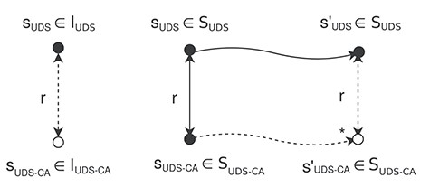
The binary relation |$r$| is a simulation from |$M_{UDS}$| to |$M_{UDS\mbox{-}CA}$|.
Condition 1 For each |$s_{UDS}$| |$\in $| |$I_{UDS}$|, there exists |$s_{UDS\mbox{-}CA}$| |$\in $| |$I_{UDS\mbox{-}CA}$| such that |$r$| (|$s_{UDS}$|, |$s_{UDS\mbox{-}CA}$|)
Proof. Let |$s_{UDS\mbox{-}CA}$| be T-Init(|$s_{UDS}$|). From the T-Init requirement, we have |$f$|(T-Init(|$s_{UDS}$|)) = |$s_{UDS}$|. This means |$f$|(|$s_{UDS\mbox{-}CA}$|) = |$s_{UDS}$|. Then, we have |$r$| (|$s_{UDS}$|, |$s_{UDS\mbox{-}CA}$|). This condition is satisfied.
Condition 2 For each |$s_{UDS}$| |$\in $| |$S_{UDS}$| and |$s_{UDS\mbox{-}CA}$| |$\in $| |$S_{UDS\mbox{-}CA}$|, |$s^{\prime}_{UDS}$| |$\in $| |$S_{UDS}$| such that |$r$|(|$s_{UDS}$|, |$s_{UDS\mbox{-}CA}$|) and |$s_{UDS}$| |$\leadsto $| |$s^{\prime}_{UDS}$|, there exists |$s^{\prime}_{UDS\mbox{-}CA}$| such that |$s_{UDS\mbox{-}CA}$| |$\leadsto ^*$| |$s^{\prime}_{UDS\mbox{-}CA}$| and |$r$|(|$s^{\prime}_{UDS}$|, |$s^{\prime}_{UDS\mbox{-}CA}$|).
Proof. Because of |$r$|(|$s_{UDS}$|, |$s_{UDS\mbox{-}CA}$|), we have |$s_{UDS}$| = |$f$|(|$s_{UDS\mbox{-}CA}$|). Let us assume that |$s_{UDS}$| |$\leadsto $| |$s_{UDS}$| by a rule |$rl$| of a UDS. According to the T-Trans-UDS&CA(2) requirement, there must be a rule |$rl^{\prime}$| of the UDS-CA converted from |$rl$| that applies to |$s_{UDS\mbox{-}CA}$| such that |$s_{UDS\mbox{-}CA}$| |$\leadsto $| |$s^{\prime}_{UDS\mbox{-}CA}$| by |$rl^{\prime}$| and |$f$|(|$s^{\prime}_{UDS\mbox{-}CA}$|) = |$s^{\prime}_{UDS}$|. |$f$|(|$s^{\prime}_{UDS\mbox{-}CA}$|) = |$s^{\prime}_{UDS}$| means |$r$|(|$s^{\prime}_{UDS}$|, |$s^{\prime}_{UDS\mbox{-}CA}$|). Then, this condition is satisfied. Since two conditions are proved, |$r$| is a simulation relation from |$M_{UDS}$| to |$M_{UDS\mbox{-}CA}$|.
The same strategy is used to prove that |$r$| is a simulation relation from |$M_{UDS\mbox{-}CA}$| to |$M_{UDS}$|.
Condition 1 For each |$s_{UDS\mbox{-}CA}$| |$\in $| |$I_{UDS\mbox{-}CA}$|, there exists |$s_{UDS}$| |$\in $| |$I_{UDS}$| such that |$r$|(|$s_{UDS}$|, |$s_{UDS\mbox{-}CA}$|).
Proof. Since |$I_{UDS\mbox{-}CA}$| contains only initial states converted from the one of a UDS. For each |$s_{UDS\mbox{-}CA}$| |$\in $| |$I_{UDS\mbox{-}CA}$|, there exists |$s_{UDS}$| = |$f$|(|$s_{UDS\mbox{-}CA}$|) |$\in $| |$I_{UDS}$|. This means |$r$|(|$s_{UDS}$|, |$s_{UDS\mbox{-}CA}$|). This condition is satisfied.
Condition 2 For each |$s_{UDS\mbox{-}CA}$| |$\in $| |$S_{UDS\mbox{-}CA}$| and |$s_{UDS}$| |$\in $| |$S_{UDS}$|, |$s^{\prime}_{UDS\mbox{-}CA}$| |$\in $| |$S_{UDS\mbox{-}CA}$| such that |$r$|(|$s_{UDS}$|, |$s_{UDS\mbox{-}CA}$|) and |$s_{UDS\mbox{-}CA}$| |$\leadsto $| |$s^{\prime}_{UDS\mbox{-}CA}$|, there exists |$s^{\prime}_{UDS}$| such that |$s_{UDS}$| |$\leadsto ^*$| |$s^{\prime}_{UDS}$| and |$r$|(|$s^{\prime}_{UDS}$|, |$s^{\prime}_{UDS\mbox{-}CA}$|).
Proof. The transitions of |$M_{UDS\mbox{-}CA}$| are largely classified into two groups: the UDS-CA and CA, which are as the following cases corresponding to the requirements T-Trans-UDS&CA(1) and T-Trans-CA of the function T-Trans.
(1) |$s_{UDS\mbox{-}CA}$| |$\leadsto $| |$s^{\prime}_{UDS\mbox{-}CA}$| such that |$f$|(|$s_{UDS\mbox{-}CA}$|) |$\neq $| |$f$|(|$s^{\prime}_{UDS\mbox{-}CA}$|)
(2) |$s_{UDS\mbox{-}CA}$| |$\leadsto $| |$s^{\prime}_{UDS\mbox{-}CA}$| such that |$f$|(|$s_{UDS\mbox{-}CA}$|) = |$f$|(|$s^{\prime}_{UDS\mbox{-}CA}$|)
The proof shows for each case.
(1) Let |$s^{\prime}_{UDS}$| be |$f$|(|$s^{\prime}_{UDS\mbox{-}CA}$|). This simply means |$r$|(|$s^{\prime}_{UDS}$|, |$s^{\prime}_{UDS\mbox{-}CA}$|) (*). Because of |$r$|(|$s_{UDS}$|, |$s_{UDS\mbox{-}CA}$|), we have |$s_{UDS}$| = |$f$|(|$s_{UDS\mbox{-}CA}$|). Each transitions in the UDS-CA is conducted from a transitions in |$M_{UDS}$| by the function T-Trans. In deed, the transitions |$s_{UDS\mbox{-}CA}$| |$\leadsto $| |$s^{\prime}_{UDS\mbox{-}CA}$| is conducted from |$f$|(|$s_{UDS\mbox{-}CA}$|) |$\leadsto $| |$f$|(|$s^{\prime}_{UDS\mbox{-}CA}$|) corresponding to the T-Trans-UDS&CA(1) requirement. Because |$s_{UDS}$| = |$f$|(|$s_{UDS\mbox{-}CA}$|) and |$s^{\prime}_{UDS}$| = |$f$|(|$s^{\prime}_{UDS\mbox{-}CA}$|), we have |$s_{UDS}$| |$\leadsto $| |$s^{\prime}_{UDS}$| (**). From (*) and (**), this condition is satisfied.
(2) The transactions in (2) never change anything used by UDS but only change control information to run CA. Let |$s^{\prime}_{UDS}$| be |$f$|(|$s^{\prime}_{UDS\mbox{-}CA}$|). We simply get |$r$|(|$s^{\prime}_{UDS}$|, |$s^{\prime}_{UDS\mbox{-}CA}$|) (*). From the assumption |$r$|(|$s_{UDS}$|, |$s_{UDS\mbox{-}CA}$|), we have |$s_{UDS}$| = |$f$|(|$s_{UDS\mbox{-}CA}$|). Because, corresponding to the T-Trans-CA requirement for such transaction, |$f$|(|$s_{UDS\mbox{-}CA}$|) = |$f$|(|$s^{\prime}_{UDS\mbox{-}CA}$|), we get |$s_{UDS}$| = |$s^{\prime}_{UDS}$|. This means |$s_{UDS}$| |$\leadsto ^*$| |$s^{\prime}_{UDS}$| (**). From (*) and (**), this condition is satisfied. Figure 7 shows these two cases.
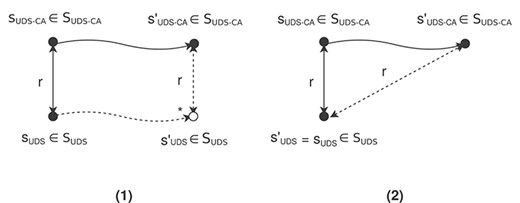
The transitions in |$T_{UDS\mbox{-}CA}$| are classified into two groups.
From what have been proved above, |$r$| is a simulation relation from |$M_{UDS\mbox{-}CA}$| to |$M_{UDS}$|. Since |$r$| is a simulation relation from |$M_{UDS}$| to |$M_{UDS\mbox{-}CA}$| and vice versa, |$r$| is a bi-simulation relation between |$M_{UDS}$| and |$M_{UDS\mbox{-}CA}$|. This states that the meta-program T preserves the behavior of a UDS.
It is necessary to prove that a meta-program satisfies all the T-State, T-Init, T-Trans-UDS&CA(1), T-Trans-UDS&CA(2) and T-Trans-CA requirements. The requirements can be checked once the complete specification of the meta-program is available.
4.2 Model checking
We model check that UDSs-FCA for some UDSs enjoy the termination property that whenever the observer claims that the UDS has terminated, it has certainly done. We define the predicate unTerm that judges whether a UDS has terminated or not. metaSearch tries to find any reachable state in which the observer claims that the UDS has terminated, but actually it has not. If there is no such reachable state, the UDS-CA satisfies the property. Otherwise, it is not. For the latter case, a counterexample will be shown.
4.3 Experiments
Let us consider the following two UDSs. The first is the system specified in Section 3.1 (shown in Fig. 3) and the second is a different one in which each process has three statuses |$\textrm{ps1}$|, |$\textrm{ps2}$| and |$\textrm{ps3}$|. In the second system, a process can change its status when it sends or receives a message. The state transitions of a process are depicted in Fig. 8a. When a process is |$\textrm{active}$|, it can send messages. Then, after sending messages, it turns to |$\textrm{passive}$| mode. The concrete system in Fig. 8b, as an example, consists of three processes. Initially all processes are in the status |$\textrm{ps1}$| and only |$\textrm{p}$| is |$\textrm{active}$|. The two underlying systems are specified as the modules SYS1 and SYS2, respectively, and T takes each module and generates T(SYS1) and T(SYS2) as the specifications of the two UDS-FCAs.
The state-transition diagram of a process and a 3-process and 6-channel system.
As a result of our model checking, counterexamples are found. This implies that the FAC does not work correctly.
Intuitively, the observer cannot conclude from S = R that the computation has terminated. This is due to the asynchrony of the communication. All processes may not receive or reply to the observer’s request at the same time. According to the counterexample for SYS1, |$\textrm{p}$| receives a request after it sends token |$\textrm{t1}$| to |$\textrm{q}$| and becomes |$\textrm{passive}$|. It sends |$\textrm{(p,1,0)}$| back to the observer. |$\textrm{q}$| receives a request before receiving |$\textrm{t1}$| from |$\textrm{p}$|. It sends |$\textrm{(q, 0, 0)}$| back to the observer. It then sends |$\textrm{t1}$| to |$\textrm{p}$| and |$\textrm{t2}$| to |$\textrm{r}$|. |$\textrm{r}$| receives a request after it receives and consumes |$\textrm{t2}$| and then it sends |$\textrm{(r,0,1)}$| back to the observer. The observer counts the numbers of messages sent and received, since it has already received all the answers from the three processes. Since |$S$| = 1 and |$R$| = 1, the observer claims that the system has terminated, when in fact the computation has not terminated because the channel from |$\textrm{q}$| to |$\textrm{p}$| is carrying |$\textrm{t1}$|. Counterexamples were also found for T(SYS2).
5 Model Checking for All Possible Initial States
Even for a fixed number of each kind of entities, such as processes, there may be multiple initial states and some initial states may lead to a counterexample for a property, while some may not. It is better to perform model checking experiments for as many initial states as possible as shown in Fig. 9a. However, it is exhausting and mistake prone to generate all possible initial states of a system and manually perform model checking experiments for them.
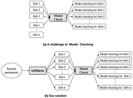
A challenge of model checking and our solution for handling many initial states.
It is sufficient to use some parameters, such as the number of processes, to systematically generate all initial states of a system such that some conditions are fulfilled, e.g. that the network is fully connected. The idea is illustrated in Fig. 9b. For a system that has, say, three fully connected processes and three tokens, all possible initial states are shown in Fig. 10. For another system that has three partially connected processes and four channels, some possible initial states are shown in Fig. 11. Note that all processes in these systems play the same role.
All possible initial states of a fully connected system.
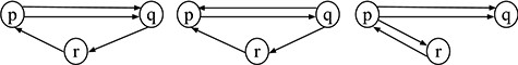
Some possible initial states of a partially connected system.
Many existing model checkers automatically take into account all possible initial states in that for a set of possible initial values, say {0, 1, 2}, of each variable, say |$x$|, all three cases such that |$x$| is 0, |$x$| is 1 and |$x$| is 2 are considered. It is not sufficient to specify the number of some entities, such as nodes and links. We also need to consider the network topologies since the network topology is a crucial factor that affects the model checking result. To the best of our knowledge, there is no existing model checker that automatically considers all or multiple network topologies for the number of nodes and links. The proposed technique does so.
For example, for the UDSs of FCA, the function to generate all such initial states could be implemented to take the number of processes and the number of tokens and return all possible initial states of the system.

where |$\texttt{ConfigSet}$| is the sort for system configuration soups.
Next, conduct model checking experiments for all of them with |$\texttt{checkAll}$| defined as follows:

where |$\texttt{CounterSet}$| is the sort for counterexample soups. |$\texttt{checkAll}$| first calls |$\texttt{InitGen}$| to generate all initial states for given parameters and then performs model checking for all. It is more likely that a CA will enjoy a desired property if no counterexample is found for any of these initial states. If the time taken is taken into account and it is sufficient to detect only one counterexample, |$\texttt{checkAll}$| could be modified so that we can stop model checking as soon as a counterexample is found.
We conduct experiments for six underlying systems described by the numbers of processes and tokens, as shown in Table 1. The number of all possible initial states for each system is presented in the fourth column. Consider the system that contains three processes and two tokens. Some possible initial states of the systems are shown in Fig. 12. We have shown in the previous section that a counterexample is found when we perform model checking for the initial state (a). However, no counterexample is found when we model checking for the initial state (b). In general, a counterexample may occur in some initial states but not in others. Suppose we perform model checking only for (b) but not (a), the counterexample is not found and the error is not detected. The experimental results are shown in Table. 1. The fifth column shows the numbers of initial states from which the counterexample is found. Also, the times taken to find the first counterexample for these initial states are given in the time taken column.
Results of the nine model checkings for FCA.
| System | Number of processes | Number of tokens | All initial states | Counter-initial states | Time-taken (minutes) |
|---|---|---|---|---|---|
| Sys 1 | 2 | 2 | 3 | 1 | 0.001 |
| Sys 2 | 3 | 2 | 5 | 2 | 5.563 |
| Sys 3 | 3 | 3 | 14 | 5 | 35.867 |
| Sys 4 | 3 | 4 | 38 | 16 | 49.765 |
| Sys 5 | 4 | 2 | 7 | 2 | 62.378 |
| Sys 6 | 4 | 3 | 19 | 7 | 158.459 |
| Sys 7 | 5 | 2 | 12 | 4 | 204.845 |
| Sys 8 | 5 | 4 | 72 | 28 | 421.642 |
| Sys 9 | 6 | 3 | 31 | 10 | 642.851 |
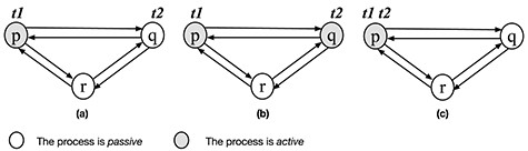
Some initial states of the system with three processes and two tokens.
In summary, checking all possible initial states of a system increases the capacity of counterexample finding or improves the confidence in the correctness of an algorithm. Another example demonstrating this point is shown in Section 7.
6 case study 1: Distributed Snapshot Algorithms
This section summarizes the research reported in [11] that specifies and model checks Chandy–Lamport algorithm (CLDSA) [22]. A UDS consists of a finite set of processes that are connected and communicated by channels that are unbounded reliable queues (FIFO). The state of a channel is characterized by the sequence of in-trans messages sent along the channel and not yet received by the destination process. CLDSA works by using a control message called marker that guides a process when it should record its state and the states of all of its incoming channels. The global snapshot then is collected by combining those recorded process and channel states.
The algorithm should satisfy distributed snapshot reachability (DSR) property as follows. Let |$s_1$|, |$s_*$| and |$s_2$| be the state in which the algorithm initiates (the start state), the snapshot taken and the state in which the algorithm terminates (the finish state), respectively. |$s_*$| is reachable from |$s_1$| and |$s_2$| is reachable from |$s_*$|, whenever the algorithm terminates. Note that |$s_1$|, |$s_2$| and |$s_*$| are states of the UDS but not those of the UDS-CLDSA. The property relates to two different systems: a UDS and the UDS-CLDSA. It is not straightforward to express the property in typical existing temporal logics, such as LTL. This is because the semantics of such a logic is defined for a single system formalized as a Kripke structure (an extension of a state machine).
Let Msg be the sort for messages and the supersort of Token. The state of a channel is expressed as a queue of messages for which the sort MsgQueue is used. The empty queue of messages is denoted as empQueue. A queue of |$n$| messages |$m_0,m_1, \dots , m_{n-1}$| in this order is denoted as |$m_0$| |$\mid $| |$m_1$| |$\mid $| … |$\mid $| |$m_{n-1}$| |$\mid $| empQueue. Process states and channel states are expressed as observable components for which the sort OCom is used: (p-state[|$p$|]: |$ts$|) for process, where p-state[|$p$|]: is the name, |$p$| is a process and |$ts$| is the value, which is a token soup and (c-state[|$p$|,|$q$|,|$n$|]: |$ms$|) for channel, where c-state[|$p$|,|$p$|,|$n$|]: is the name, |$p$| and |$q$| are the source and destination processes, |$n$| is a natural number used to identify the channel because there may be more than one channel from |$p$| to |$q$| and |$ms$| is the value that is a message queue. A system state is expressed as the soup of the observable components for which the sort Config is used.
Due to the working of CLDSA, the messages in the UDS-CLDSA contain not only data messages as in a UDS but also control messages called markers. Moreover, to describe the system, we need to express more information, such as the start state, the snapshot, the finish state and the information to control behaviors of the algorithm. Therefore, we need to use new notations to express the states of the system. For example, when CLDSA is executed in the above token system, there are not only tokens but also markers on the channels. So we need to use a new sort MMsg to denote tokens and markers and the sort MMsgQueue to denote the queues of messages of the UDS-CLDSA. The sort MMsg and MMsgQueue are the super-sorts of the sort Msg and the MMsgQueue, respectively. The new sort to denote observable components and the soup of them are BOCam and BConfig, respectively. The states of the UDS-CLDSA are expressed as follows:

where bc, sc, ssc, fc and ctl are terms that describe the state of processes and channels, the start state, the snapshot, the finish state and the information to control behaviors of the algorithm, respectively.
As the description of our approach, CLDSA is specified as a meta-program (cl). A UDS is specified as a module and then cl transfers it to the UDS-CLDSA.
The function |$f$|. Since CLDSA uses a control message marker, the state of a channel contain not only message, manely |$token$|, but also |$marker$|. The function T-State revises observation components of a UDS and add new observation components. Let delMarker be the function that takes a value of the sort MMsgQueue and returns a value of the sort MsgQueue. Namely, delMarker deletes all markers in the queue. The function |$f_i$| is specified as f-i in Maude as follows.

Let fg-i be the function that applys f-i to all observation components of a term of the sort BOCom. It is recursively defined as follows:

The function |$f$| is specified as follows:

Basically, the function |$f$| reverses all observation components related to those of a UDS by deleting all markers in the state of a channel and getting rid of new observation components. We invite readers to read the paper [13], in which we prove that the formal specification of CLDSA preserves a given UDS by what is described.
A faithful formal definition of the property has been given in [13]. It is checked that CLDSA is terminated in the UDS-CLDSA, but it is checked that some states of a UDS are reachable from some others in the UDS but not the UDS-CLDSA. We propose a new model checking method by which a counterexample is shown when the algorithm does not enjoy a property. Our method directly deals with the faithful formal definition of the property.
We compare the performance of our proposed method with an existing one [31]. We conduct model checking for eight different systems. The results of experiments have shown that our proposed approach surpasses in performance the existing one. For the details of how to specify, model checking and experiments, we invite readers to read the published paper [11].
7 CASE STUDY 2: Checkpointing Algorithms
Checkpointing, an essential technique for fault tolerance distributed systems, helps reduce the amount of lost work by periodically saving the state of a process during fault-prone execution. The saved state of a process is called a local checkpoint and a global checkpoint is a set of local checkpoints, one from each process.
7.1 Underlying mobile distributed systems
A mobile computing system consists of a set of MHs that can move and a set of MSSs that act as access points to connect the MHs to the rest of the network. MSSs communicate with other MSSs over wired networks that provide reliable messaging, but with MHs over wireless networks. The location of an MH is represented by its current local MSS. The system shown in Fig. 13 consists of three MSSs and seven MHs. Due to the mobility of an MH, it may connect to different MSSs from time to time. An MH can disconnect from the network voluntarily. An MH passes messages in a reliable FIFO wireless channel to communicate with an MSS when it locates in the coverage of the MSS (called |$cell$|).
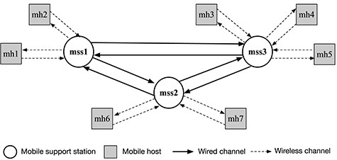
A mobile distributed system consisting of three MSSs and seven MHs.
7.2 Mutable checkpointing algorithm
Cao and Singhal [6] proposed a coordinated checkpointing algorithm (referred as CP), where only a minimal number of processes need to take their checkpoints on the stable storage. The concept of ‘mutable checkpoints’ is introduced. A mutable checkpoint is neither a tentative checkpoint nor a permanent checkpoint but can be turned into a tentative checkpoint at some points. CP requires that each |$p_i$| of MHs and MSSs stores the following pieces of information (let |$n$| be the total number of MHs and MSSs):
|$\bullet $| |$R_i$|: an array of bits such that its size is |$n$|. |$R_i[j]$| = 1 means that |$p_i$| has received computation messages from |$p_j$| in the current checkpointing interval.
|$\bullet $| |$csm_i$|: an array of checkpoint numbers such that its size is |$n$|. |$csm_i[j]$| represents the checkpoint number of |$p_j$| that |$p_i$| knows.
|$\bullet $| |$weight_i$|: a non-negative number whose maximum value is 1. It is used to detect the termination of the algorithm.
|$\bullet $| |$trigger_i$|: a pair (|$pid$|, |$imun$|); |$pid$| is the identifier of the last checkpoint initiator for which |$p_i$| has processed the request and |$imun$| is the checkpoint number of the initiator.
|$\bullet $| |$sent_i$|: a Boolean that is set to 1 if |$p_i$| has sent messages in the current checkpoint.
|$\bullet $| |$cp\mbox{-}state_i$|: a Boolean that is set to 1 if |$p_i$| is in the current checkpoint.
|$\bullet $| |$old\mbox{-}csm_i$|: the checkpoint number of the current tentative checkpoint.
|$\bullet $| |$Cp_i$|: a tuple to store the mutual checkpoint.
|$\bullet $| |$Mr_i$|: an array storing inheritance information. An element |$Mr_i[k]$| is a structure containing two numbers |$csm$| and |$R$| (|$Mr_i[k].csn$| and |$Mr_i[k].R$|).
|$p_i$| could start CP at any time when it is not in any checkpoint process. It takes its local checkpoint, increments its |$csm_i[i]$|, sets |$weight_i$| to 1 and |$cp\mbox{-}state_i$| to 1 and stores its own identification and the |$csm_i[i]$| to |$trigger_i$|. It then sends checkpoint requests to all its relative components |$p_j$| such that |$R_i[j]$| =1 (meaning that |$p_i$| has received messages from |$p_j$|). When |$p_i$| receives a checkpoint request, it checks whether it must inherit the request. If it does not, it sends a reply to the initiator. Otherwise, it handles the request: it either takes a new local checkpoint or makes the mutual checkpoint tentative, sends a response message to the initiator and then propagates the request to all its relatives. When |$p_i$| sends a computation message, it adds more information (its own |$csm_i[i]$| and |$trigger_i$|) to the message if it is in a checkpoint process. Each component that receives a computation message checks whether or not it needs to take a mutual checkpoint or not. A mutual checkpoint becomes tentative when the component receives a checkpoint request. Otherwise, the mutual checkpoint is discarded. When an initiator receives all replies from its relative components, it announces the termination of the checkpoint process and sends a broadcast message to all components in the system. The details of CP can be found in [6].
7.3 Specification of underlying mobile distributed systems
Syntax part. There are three observable components in the systems: MHs, MSSs and channels. A message is expressed as (|$p, q, d$|), where |$p$| is the source process, |$q$| is the destination process and |$d$| is the data. The three observable components are as follows: |$< [mb: loc, cos ]>$| for mobile hosts, where the name |$mb$| is its identification and the value ‘|$loc, cos$|’ consists of its local state and its connection state, |$mss: mbl, ms$| for stations, where the name |$mss$| is its identification and the value ‘|$mbl$|, |$ds$|’ consists of the set of mobile identifications associated with it and the queue of incoming messages, and [|$sp,ds: st$|] for channels, where the name ‘|$sp,ds$|’ consists of the source and destination, and the value |$st$| is its state. The state of a system is a soup of observable components.
Transition part. An MH can perform three kinds of actions: (i) sending messages, (ii) receiving messages and (iii) disconnecting or reconnecting to the network. All actions are specified as rules. For example, the following rule specifies the action when a mobile host sends a computation message to another mobile host that is in a different cell by sending the message to its local station:

where the variables are MB1, MB2 for mobile identifications, MSS1, MSS2 for station identifications, CS1, CS2 for mobiles states, D for data, C for a soup of observable components, LMS for queues of messages and MS for messages.
Let cp be the meta-program as a formal specification.
cp-State. There are three kinds of control messages: ‘request,’ ‘reply’ and ‘broadcast’ messages, which contain information that must be exchanged by components to execute CP.
Because a computation message sent by |$p_i$| must contain more information, namely |$csm_i[i]$| and |$trigger_i$|, a new form of computation messages, which are called meta-computation messages is utilized. Both control messages and meta-computation messages are called meta-messages. Thus, the expressions of the local states of the mobile, station and channel are different from those of a UMDS.
Some pieces of information needs to be added to each observable component of the mobile (or station). Such revised observable components are called meta-observable components and are expressed in the form of m-pro(|$ms$| |$ar$| |$cs$| |$we$| |$tr$| |$se$| |$cs$| |$ol$| |$cp$| |$ms1$| |$ms2$| |$cS$|), where |$ms$| is an observable component (mobile or station), |$ar$|, |$cs$|, |$we$|, |$tr$|, |$se$|, |$cs$|, |$ol$| and |$cp$| are |$R_i$|, |$csm_i$|, |$weight_i$|, |$trigger_i$|, |$sent_i$|, |$cp\mbox{-}state_i$|, |$old\mbox{-}csm_i$| and |$Cp_i$|, respectively, |$ms1$| and |$ms2$| are soups of messages sent and received by the component and |$cS$| is a list of tentative checkpoints. The meta-observable component of a channel has the form of m-chan(|$cn$|), where |$cn$| is an observable component (channel). A global state of a UMDS-CP is expressed as a soup of meta-observable components. Some notations used in the specification of a UMDS are still used in the specification of the UMDS-CP. However, some notations are no longer used. cl-State must remove notations that are not used and add any other notations necessary to describe the UMDS-CP.
cp-Init. Each initial state of a UMDS is of the form |$<\ [mh_1\ ]>$|, …, |$<\ [mh_n\ ]>$|, |$\{mss_1\}$|, …, |$\{mss_m\}$|, |$[cn_1]$|, …, |$[cn_k]$|, where each |$<\ [mh_i\ ]>$|, |$\{mss_j\}$| and |$[cn_k]$| is an observable component as described. Each initial local state of MH (or MSS) in the UMDS-CP is the same as that of the UMDS, but we need to add any other necessary meta-observable components that have the corresponding initial values. The corresponding initial state of the UMDS-CP is |$m\mbox{-}pro(<\ [mh_1\ ]>$| |$MC_1)$|, …, |$m\mbox{-}pro(<\ [mh_n\ ]>$| |$ MC_n)$|, |$m\mbox{-}pro(\{mss_1\}$| |$SC_1)$|, …, |$m\mbox{-}pro(\{mss_m\}$| |$SC_m)$|, |$m\mbox{-}chan\ [(\ ][\ [cn_1\ ]])$|, …, |$m\mbox{-}chan\ [(\ ][\ [cn_k\ ]])$|, where |$MC_1$|,…, |$MC_n$| and |$SC_3$|, …, |$SC_n$| are terms in which control information is initialized. cp-Init converts each initial configuration for a UMDS into one for the UMDS-CP.
cp-Trans. The rules of the UMDS-CP are classified into two parts: UMDS&CP and CP. For example, in the UMDS&CP part, the following is such a rule:

The rule is generated from the rule sendMobile of the UMDS. When an MH sends the messages to its local MSS, it changes the value of |$sent$| to ‘1’ (expressed as (Sent: 1) on the right-hand side of the above rule, while it is (Sent: N2) on the left-hand side, where N2 may not be 1), which means that the MH has sent messages. Such a message contains not only the computation information but also the information about its |$csm_i[i]$| and |$trigger_i$|, which are expressed as N1 attached in (NB1, N1) and TR1, where i = MB1. Note that an array |$a$| is formalized as a soup of pairs |$(i, v)$|, where |$i$| is an index and |$v$| is the value |$a[i]$|.
cp-Trans takes each rule of a UMDS and modifies it. For instance, ¡ MB1, D CS1, MSS1 ¿ changes to m-pro( ¡ MB1, D CS1, MSS1 ¿ R1 CSM[(MB1, N1) LPC] W1 TR1 (Sent: N2) (CP-state: 0) OLD1 CP1 CM1 CM2 CL1). ¡ MB1, D CS1, MSS1 ¿ is kept, while the other part is not dependent on the state of the UMDS. cl-Trans then adds all rules of the CP part.
7.4 Model checking
7.4.1 Model a desired property
A checkpointing algorithm must guarantee that each recorded global checkpoint is consistent. A consistent checkpoint must not contain an |$orphan$| message sent by a process after it has taken its local checkpoint but recorded by another process as a received message in its local checkpoint. We define the predicate checkInCons that evaluates whether an orphan message is present in a checkpoint. The model checking is performed by using metaSearch to find any current checkpoint that contains an |$orphan$| message. If the search finds such a current checkpoints, then CP does not satisfy the property.
7.4.2 Generating and model checking of all possible systems
The topology of the wired network could affect the routing of messages in the system. Therefore, it is necessary to check CP for the different wired network topologies. Note that for two stations |$mss1$| and |$mss2$|, if there is a channel from |$mss1$| to |$mss2$|, there is always another channel from |$mss2$| to |$mss1$|. Considering a system in which there are a fixed number of MHs and a fixed number of MSSs, there are many possible initial states due to the wired channels between the MSSs. For example, in a system with four MSSs and four MHs, some possible initial states of the system are as shown in Fig. 14. We define the function cp-IniGene, which takes the numbers of MHs and MSSs and generates all possible initial states. We use the constraint that the MSSs are |$strongly$| connected to wired channels to keep the number of generated initial states moderate. To conduct experiments for this case study, we define the function cp-checkAll to stop at the first initial state in which a counterexample is found.
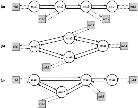
Some possible initial states of a mobile distributed system consisting of four MSSs and four MHs.
7.5 Experiments
We have conducted model checking for some different UMDSs. As a result of model checking, counterexamples are found. Analyzing these counterexamples, we find a minor error in the pseudo-code of CP, which is as follows. If |$p_i$| propagates the request to all components on which it depends on, this may result in a large number of redundant system messages. The designers of CP solve this problem by appending some information stored in |$Mr_i$| to the request. If |$p_i$| knows (by checking |$Mr_i$|) that |$p_k$| on which it depends has received the request from another component, |$p_i$| does not send the request to |$p_k$|. The idea is implemented in the procedure prop-cp in the pseudo-code. |$p_i$| sends the request to |$p_k$| iff |$R_{i}[k]$| equals |$1$| (meaning that |$p_i$| depends on |$p_k$|) and |$csm_{i}[k]$| is greater than |$Mr_i[k].csm$| (meaning that |$p_k$| has not received the request from other components). Unfortunately, the algorithm malfunctions. Let us consider the following case. Based on CP, |$cms_{i}[k]$| is initially set to |$0$|. Assuming that |$p_i$| has received a computation message from |$p_k$| (|$R_{i}[k]$| is set to |$1$|). |$p_i$| then starts CP. It sets |$Mr_i[k].csm$| to |$0$|. Because |$p_i$| depends on |$p_k$| and |$p_k$| has not received the request, |$p_i$| should send the request to |$p_k$|. However, according to CP, the request is sent iff |$R_{i}[k]$| equals |$1$| and |$csm_{i}[k]$| is greater than |$Mr_i[k].csm$|. Thus, |$p_i$| does not send the request to |$p_k$| because both |$csm_{i}[k]$| and |$Mr_i[k].csm$| equal |$0$|. This error could be fixed as follows. When |$p_i$| starts CP, |$p_i$| sends the request to |$p_k$| iff |$R_{i}[k]$| equals |$1$| and |$csm_{i}[k]$| is greater than |$Mr_i[k].csm$| or both |$csm_{i}[k]$| and |$Mr_i[k].csm$| equal |$0$|.
The above counterexample occurs in the model checking of any initial state. However, we will show another error that demonstrates the usefulness of our method for generating and model checking all possible initial states. Because we have found the source of the first error, we fix the error, rerun the model checking and find another error. We performed experiments for six instances of the system described by the numbers of MSSs and MHs as shown in Table 2. The second column presents the number of MSSs, the third column presents the number of MHs and the number of all possible initial states is shown in the fourth column.2
Results of the six model checkings for CP.
| Sys | MSS | MH | All | Initial states 1 | Time taken 1 | Initial states 2 | Time taken 2 |
|---|---|---|---|---|---|---|---|
| S1 | 3 | 3 | 2 | 2 | 0.507 | N/C | 0.000 |
| S2 | 3 | 5 | 3 | 3 | 3.617 | N/C | 0.000 |
| S3 | 4 | 4 | 10 | 10 | 5.867 | 3 | 65.633 |
| S4 | 4 | 6 | 16 | 16 | 19.453 | 3 | 265.986 |
| S5 | 5 | 5 | 148 | 148 | 22.341 | 52 | 305.657 |
| S6 | 5 | 8 | 186 | 186 | 57.559 | 74 | 562.393 |
Considering a very simple mobile system with four MSSs and four MHs, there are many possible initial states of the system and some of them are as shown in Fig. 14. Let us focus only on the two initial states |$\textbf{(a)}$| and |$\textbf{(b)}$| and consider two MHs |$mb1$| and |$mb4$|. In |$\textbf{(a)}$|, when |$mb1$| sends a message to |$mb4$|, there is only one route to pass the message from |$mb1$| to |$mb4$| through |$mss1$|, |$mss2$|, |$mss3$| and |$mss4$|, while in |$\textbf{(b)}$|, there are two routes to pass the message either through |$mss1$|, |$mss2$| and |$mss4$| (route1) or |$mss1$|, |$mss3$| and |$mss4$| (route2). Suppose that |$mb1$| has received computation messages from some other components but not yet from |$mb4$|. It starts the first checkpointing process, records its local checkpoint and asks all its related components to take their local checkpoints (Fig. 15(p1)). After receiving all replies from these components, it terminates the checkpoint process and sends broadcast messages to all components in the system, including |$mb4$|. The message, e.g. |$bms$|, is passed to |$mb4$| via the route 1 (Fig. 15(p2)). It may happen that while the broadcast message is on its way to |$mb4$|, |$mb4$| sends a computation message to |$mb1$| and |$mb1$| then starts the second checkpoint process. Thus, it sends the checkpoint request, e.g. |$rms$|, to |$mb4$|. We assume that the request is delivered to |$mb4$| via the other route2 (Fig. 15(p3)). When |$mb4$| receives the request, it takes its local checkpoint and sends a reply to |$mb1$| (Fig. 15(p4)). The broadcast message now arrives at |$mb4$|. According to the algorithm pseudo-code, |$mb4$| terminates the checkpoint process by setting the |$cp\mbox{-}state_{mb4}$| to |$0$| (Fig. 15(p5)). This is an error because the broadcast message corresponds to the first checkpoint but not the current checkpoint. It occurs because there are two different routes to pass a message from |$mb1$| to |$mb4$|. The checkpoint request of the second checkpoint process arrives before the broadcast message. This counterexample is found when we model check the initial state as in |$\textbf{(b)}$|. However, in the initial state |$\textbf{(a)}$|, this counterexample does not occur because there is only one route from |$mb1$| to |$mb4$|. The broadcast message definitely arrives at |$mb4$| before the checkpoint request. The error is very simple and can be fixed by checking whether the broadcast message corresponds to the current checkpoint of a component. When |$p_i$| receives a broadcast message, it compares |$trigger_i$| and the message |$trigger$|. If they match, it terminates its checkpoint process; otherwise, it rejects the message. However, the point is that a counterexample may occur in some initial configurations but may not in the others. Thus, if we perform model checking only for configurations as in |$\textbf{(a)}$|, the counterexample cannot be found. It is almost impossible for humans to predict all cases in advance. Fortunately, by generating all possible initial states, our method enables the discovery of counterexamples lurking in the UMDS-CPs for the property concerned. In the other words, it increases the counterexample detection rate or the correctness confidence of an algorithm. The proposed technique allows to handle a case when a CA manages two or more underlying systems. A UDS is essentially formalized as a directed graph. The proposed technique can deal with a graph that has two or more disconnected components. Each disconnected component can be considered as an independent UDS.
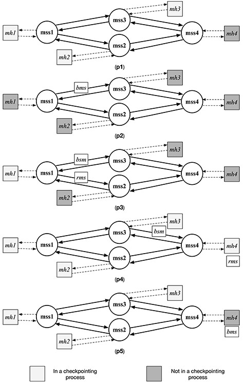
The counterexample found for the initial state (b).
Table 2 shows the results of the model checking experiments. The fifth column of the table shows the number of initial states from which the counterexample of the first error is found, and N/C means that the counterexample is not found in any initial state. The next column shows the time taken to find the counterexample. In the same meaning, the last two columns show the number of initial states and the time taken to find the counterexample of the second error.
8 Conclusion
We have proposed (i) a technique that specifies a distributed CA as a meta-program that takes a specification of an UDS and automatically generates the specification of the UDS on which the CA is superimposed (UDS-CA). We have also proposed (ii) a technique that can model check if the UDS-CA generated as just mentioned enjoys desired properties that may involve not only the UDS-CA but also the UDS at the meta-level. The proposed technique makes it possible to handle a case such that one CA manages two or more underlying systems. A UDS is essentially formalized as a directed graph. The proposed technique can deal with a graph that has two or more disconnected components. Each disconnected component can be regarded as an independent UDS.
Moreover, we have proposed (iii) a technique that takes the number of each kind of entities used, generates all possible initial states for the given number of each kind of entities and conducts model checking experiments for all the initial states. Even fixing the number of each kind of entities used by a UDS, there may be more than one initial state because of, for example, the topology of the network used by the UDS. Technique (iii) makes it more likely to detect a subtle flaw lurking in a CA. The CLDSA and the Cao–Singhl mobile checkpointing algorithm (CP) have been used to demonstrate the usefulness of technique (i). One desired property CLDSA should enjoy is what is called the DSR property that involves both a UDS and the UDS-CLDSA, which has been used to demonstrate the usefulness of technique (ii). For one desired property CP should enjoy, a counterexample is found for some initial states but not for the others even by fixing the numbers of MHs and MSSs, which has been used to demonstrate the usefulness of technique (iii). Liu et al. [17] propose a technique similar to (iii) but their technique does not take into account network topologies.
Although technique (iii) is useful as demonstrated, it causes another challenge because a huge number of initial states may be generated even though we use some constraints, for example, on the network topology. There are at least two possible remedies for this challenge. Initial states may be classified into a small number of groups. One representative initial state can be taken from each group, and then we can conduct model checking for each representative initial state but not for all initial states. The other possible remedy is to use a parallel (or distributed) computing environment. Model checking experiments for multiple initial states are totally independent from each other. Therefore, multiple model checking experiments can be conducted simultaneously. It is our future work to investigate the two possible remedies for a huge number of initial states.
As mentioned, it is not very hard to check if a meta-program, the formal specification of a CA, conforms to the requirements of T-State, T-Init and T-Trans, but it would be preferable to build a tool that automatically check if a given meta-program, the formal specification of a CA, conforms to the requirements. This is one piece of our future work.
DATA AVAILABILITY STATEMENT
The data underlying this article are available at https://doi.org/10.6084/m9.figshare.15088131.v1.
FUNDING
Japan Society for the Promotion of Science (JP19H04082).
Footnotes
The name |$base\mbox{-}state$| may be changed in some implementations.
The experiments focus on the working of the algorithm for different wired channels among MSSs. MHs are simply assigned to MSSs such that at leat one MH is connected to an MSS and MSSs that have more channels are given higher priority to have MHs assigned.
References
