


Abstract
This article reviews different literature strands and performs empirical tests to identify new stylized facts on how capital ownership, particularly its nationality, relates to long-run economic development. The results indicate that low- and middle-income countries with larger foreign capital stock in 1980 had lower economic growth over the next four decades. The estimations also suggest that these economies developed a less specialized export basket, which became relatively more concentrated in low-tech goods. The results are inverted to high-income economies, for which the relationship is positive for GDP growth and export specialization and complexity. These stylized facts are in line with (and can be interpreted as a test to) the hypothesis proposed by Alice Amsden’s seminal book ‘The Rise of the Rest’ (2001) to explain different growth trajectories among developing countries. The results can also be interpreted in light of theoretical and empirical evidence that foreign capital might reinforce static comparative advantages in developing economies, particularly in middle-income ones.
1. Introduction
Foreign investment is frequently a matter of public interest in developing countries, being used as a parameter of the government’s economic management success: a low inflow tends to be understood as a sign that the economy is not performing well and that its future is worrisome. The logic, implicit most of the time, is that foreign investment does not only reflect the current state of the economy but is a central element in promoting growth. This position is based on the standard introductory-level economic reasoning that capital will flow to where it is relatively scarcer and, consequently, its remuneration tends to be larger; if this does not happen, it must be due, allegedly, to high risks in the domestic economy.
However, even among critics (or ‘dissents’1) of this mainstream reasoning, the expected effect of foreign capital on the domestic economy is far from consensual. According to Dani Rodrik, ‘[o]ne dollar of FDI is worth no more (and no less) than a dollar of any other kind of investment’ (Moran, 2005, p. 281). This view differs from that of Ha-Joon Chang, for instance: ‘[t]he home country appropriates the bulk of the benefits from a transnational corporation (...) the nationality of a firm is still key to deciding where its high-grade activities, such as R&D and strategizing, are going to be located (...) it would be very naive to design economic policies on the myth that capital does not have national roots’ (Chang, 2012, p. 115). Part of the seemingly conflicting positions on the matter can be attributed to the multitude of angles from which it can be addressed. Looking at the effects of foreign firms’ entrance into one particular sector in a developed country, for instance, will provide some evidence on one specific way capital ownership can matter but might tell very little about, for instance, the question this article aims at addressing: how the presence of foreign capital can impact economic development on the long-run, particularly in underdeveloped countries.
The idea that ownership matters for long-run growth is not new. In Singer (1950), for instance, the concept that the terms of trade of primary commodity producers would tend to deteriorate over time—which would become the core of the seminal Prebisch-Singer hypothesis, co-formulated by Prebisch (1950)—emerges as one particular potential effect of investment from developed economies in underdeveloped ones. Given the predominance of foreign investment in export sectors, dominated by primary goods in these less developed economies, Singer (1950) argues that the productive units associated with these investments acted as enclaves in the host country, not promoting structural changes. Moreover, the productivity gains in these sectors were not absorbed domestically but sent abroad via profits or through the worsening of trade terms. Not least important, Singer (1950, p. 476) points to the opportunity cost of such capital inflow for the host economy, which could reinforce the existing comparative advantages and discourage dynamic production complexification. To the static view of trade that focuses on short-term productivity gains from foreign investment, the author argues that ‘[w]e must compare, not what is with what was, but what is with what would have been otherwise’.
In a more recent work, Amsden (2001) discusses the convergence path that a group of developing countries took after World War II and places capital ownership differences at the centre of the argument of why some of these economies continued to catch-up after the 1980s and others stagnated. The basic idea proposed is that foreign companies invest less in innovation and that those affiliates often crowd out domestic firms in sectors with larger potential for productivity increase.
It is intriguing that despite the enormous literature that emerged in the 1990s on the determinants of economic growth and the more recent, but also influential, discussion on the middle-income trap (e.g. Agénor, 2017), the hypothesis formulated by Amsden (2001) has not been tested directly. Her work is an important reference for the article and will be resumed in Section 2 and motivate our empirical exercise in Section 3.
Most of the recent literature related to our question focuses on the short-term effects of foreign capital inflow as foreign direct investment (FDI henceforth). Although the goal of the article is to analyze the long-run effects of foreign capital stock, given the relevance of the FDI literature and that its insights can offer us elements to think about our question of interest, a significant part of Section 2 is dedicated to reviewing these works. In particular, I am interested in identifying alternative channels through which foreign capital might affect the economic structure of developing economies in the long-run in order to complement the hypothesis based on Amsden (ibid.), which focuses on differences in Research & Development (R&D) investment by domestic and foreign firms.
In Section 2, thus, I present some theoretical and historical inputs related to the potential effects of capital ownership on economies. By connecting different strands of the literature, the goal is to present a coherent hypothesis of how capital nationality might matter for long-run economic development.
In Section 3, I move to an empirical investigation of the hypothesis by checking the effects that the stock of foreign capital in 1980 had on the development of 65 countries over almost four decades. The main results, robust to a number of specifications and controls, including those common in the long-run growth literature (e.g. institutional quality, cost of investment, geographical distribution), indicate that larger foreign capital presence in developing countries is associated with lower long-run economic growth, in line with the hypothesis by Amsden (2001). I also find some evidence that in those economies, a higher share of foreign capital is associated with a less specialized export basket and with a larger share of low-tech goods. The results are inverted to high-income economies, for which the effects are positive on GDP growth and export specialization.
In econometric terms, these estimations are similar in spirit to the cross-country growth regressions that became popular in the 1990s. Interpretation of the results follows the current understanding of such techniques by not making causal claims but, instead, identifying patterns and stylized facts (e.g. Durlauf, 2009). It must be noted, however, that the most important bias in this literature—that GDP growth tends to influence the variables used to explain it; in our case, foreign investment—is at least partially avoided in this article by using only initial levels of the explanatory variable. Moreover, this bias would be positive, and since I find a negative correlation between foreign capital stock and long-run economic growth for developing economies, if there is any persistence of this bias, the results are conservative for this group of countries—that is, the true correlation between foreign capital and growth is even more negative.
Therefore, the contribution of this article is twofold. First, it aims at resuming the explanation for long-run economic growth proposed by Amsden (2001) and, by complementing it with insights from the vast theoretical and empirical literature on foreign direct investment, reformulate in more general terms the hypothesis that indigenous capital might be important for economic development. Second, I perform a simple evaluation of the hypothesis and find robust evidence in its favour. Combining the empirical results with the theoretical discussion of the effects of foreign capital entrance, it is possible to conjecture that, in the case of developing economies, foreign capital ownership might have reinforced the static comparative advantages of the host countries, crowded out local firms with potential to innovate while increased demand in backward sectors.
Besides this introduction, the article contains three other sections. Section 2 starts by reviewing the FDI literature to present the main channels through which foreign capital entrance can affect developing economies according to this literature. I then present the main argument by Amsden (2001) in greater detail to further substantiate my hypothesis and motivate the empirical test performed in Section 3. In Section 4, robustness tests for the econometric analyses are conducted. Section 5 discusses the empirical results, proposes an interpretation in light of the theoretical arguments presented, and concludes the article.
2. Foreign direct investment and a visit to ‘the Rest’
2.1 How and when FDI can affect the host economy
There are several theoretical channels through which the entrance of Foreign Direct Investment can affect the host economy. Since the resurgence of FDI in the late 1980s, the most prominent channel in political and academic spheres has been knowledge transfer; that is, the idea that multinational firms can bring productive knowledge upgrades to the host economy. In practical terms, such knowledge transfers can emerge from partnerships between the affiliate and domestic companies, from local firms ‘observing’ new products brought by the multinational, and via the labour market (rotation of workers between firms, connections between workers sharing some specific knowledge and spin-offs, for instance). These transfers can be of two types: horizontal or vertical. The former happens when the entrance of a multinational firm in a given sector promotes an increase in ‘knowledge’ and productivity in firms of the same sector, while the vertical case takes place when the affiliate entrance in a particular activity boosts the performance of firms in other, related activities—particularly in those that produce inputs used by the affiliate (e.g. Moran, 2005).
Firms tend to protect intellectual capital that provides them some market power while encouraging productivity gains in suppliers so that their costs can be reduced; that is, multinational corporations (MNCs) tend particularly to promote vertical transfers. Assuming stronger vertical linkages, there is no direct advantage for the host economy if the suppliers’ productivity gains are absorbed entirely by the affiliate via lower prices, given that the productivity increase will result exclusively in larger profits for the MNC (e.g. Alfaro et al., 2010).
The last point cited above is related to a second channel through which foreign firms’ entrance can affect the host economy: pecuniary externalities. In contrast to knowledge spillovers, pecuniary externalities take place via market transactions. These externalities can be related to backward or forward linkages. When an MNC’s operation boosts demand for inputs, creating the conditions for the production of new intermediate goods or allowing suppliers to take advantage of economies of scale, a backward linkage occurs. If the operation of the MNC reduces the costs or improves the quality of inputs for other firms and sectors, it is said to have created forward linkages.2
A third important channel through which FDI can impact local economies is the reallocation of resources. The idea is that MNCs’ entrance would increase competition in the local market for inputs and goods, promoting productivity-enhancing effects within and between firms. Within local firms, the increase in competition might force companies to focus on goods whose production is relatively more efficient and to promote improvements that reduce their gap to the technological frontier (Aghion et al., 2009); these productivity increases operate at an ‘intensive margin’ (Alfaro and Chen, 2018). In contrast, the reallocation of resources between firms works at an ‘extensive margin’. MNC’s entrance will, on the one hand, increase factor competition, increase costs, and, on the other hand, decrease domestic firms’ product prices due to higher competition in the goods market.3 Both ‘extensive margin’ effects raise the productivity threshold required for domestic firms’ survival, which forces some domestic firms to exit, augmenting the overall productivity in the economy by increasing the weights of the most productive firms in aggregate output and liberating resources to the most productive units.
Finally, a classical argument relating to Foreign Direct Investment and the host country’s economy is the accumulation of production factors, which would be more important the poorer the host country is. The focus tends to be on capital accumulation, which is seen as the limiting factor in underdeveloped economies. The ‘augmentation’ of labour via human capital, however, has gained increased importance. The latter can be affected by FDI if, for instance, multinational firms invest more in employee training (assuming that the skills learned are not specific to the firm itself).4
Before I examine the empirical evidence on these mechanisms, another relevant theoretical exploration is which circumstances affect the probability that the effects are positive or negative.
The general idea behind most of the conditions for the host economy to benefit from FDI is the same: the economy must have good competitive capacities (Moran et al., 2007), which tends to be associated with a given level of ‘absorptive capabilities’. In other words, and as already discussed by Hirschman (1971), foreign firms’ entrance tends to work as a competitive shock, which either harms the local economy and pushes local firms out of the market or stimulates domestic companies to become more productive. What determines which of the cases will follow is the economy’s capacity to respond to increased competition.
One important condition is the amount of human capital, or skilled labour, in the host economy before the FDI entrance. For the transfer of knowledge to happen, be it vertical or horizontal, a minimum set of labour capabilities is needed. A minimum amount of skilled labour is also relevant for pecuniary externalities to reach their full potential, given that the expansion of sectors backwards or forward, particularly in sectors with higher technological content, requires this type of labour. If human capital is low, the host country might not be able to absorb the knowledge at all; if skills are too concentrated in a small portion of workers, the multinational company might absorb most of it, forcing other firms that use this labour out of the market.
A second aspect central to the effects of MNCs’ entrance into the host country is the local financial market. In this case, too, there are a number of reasons for it. One is that for backward linkages to take place, some initial capital will tend to be used by those firms that produce inputs.5 A second reason is to ensure that the entrance of an MNC does not make available capital scarcer, an issue particularly problematic for underdeveloped countries. This might generate a crowding-out effect, preventing local firms from taking advantage of externalities. Still, a third reason for the relevance of well-developed financial markets in the host economy is facilitating the reallocation of capital from less to more productive companies.
2.2 Empirical evidence
In terms of empirical findings on the impact of FDI on the host economy’s productivity and growth, the net effects are, in general, ambiguous.
There is robust evidence that MNCs tend to have higher productivity than domestic firms in the same sector, even after controlling for the fact that FDI tends to flow to the more productive firms (see Arnold and Javorcik, 2009 for Indonesia, for instance). However, a vast literature, sparked by the work of Aitken and Harrison (1999), indicates that while FDI raises productivity in plants that receive the investment, it reduces in others, tending to generate negative or insignificant net (macro) effects for developing countries. There is also evidence that FDI does not tend to crowd in domestic investment in underdeveloped countries, actually crowding out in some periods and regions, particularly in Latin America (Agosin and Machado, 2005).
Meyer and Sinani (2009) present a hypothesis, supported by a meta-analysis of empirical works, that the effect of foreign firms’ entrance is not only conditional but non-linear: FDI generates positive effects for economies at the extremes of a development index. Three main factors would be determinants for such a result: income level, human capital and institutional development.6
Harrison and McMillan (2003) analyze French multinationals in Cote d’Ivoire and find that multinational firms tend to finance most of their investment locally, which leads to a crowding out of credit to local firms. In a similar article but using data from mostly high and middle-income countries, Harrison et al. (2004) find the opposite, that FDI reduces credit constraints of local firms; that is, foreign firms crowd in domestic enterprises. To reconcile these different results, the authors argue that, in general, FDI tends to increase domestic credit supply; however, in the case of countries with underdeveloped financial markets with significant market imperfections, multinational entrance may tighten financial constraints.7
In a seminal work, Borensztein et al. (1998) examined FDI flow from OECD countries to underdeveloped economies from 1970 to 1989. The authors find that FDI has a positive effect only if the level of human capital (measured by years in school) is above a given threshold; for very low levels, the effect of the FDI on growth is negative.8
Xu (2000) analyzes technology diffusion from FDI using US multinational enterprises data from 1966 to 1994. The author finds that for developed countries as hosts, FDI increases growth and is as important as international trade for technology spillovers. However, for underdeveloped economies, there is no positive technology transfer. The author finds that technology transfer is positively correlated with human capital and that there is also a threshold above which the host country must benefit from technology absorption.
There is also evidence that FDI can reinforce path-dependency in human capital. Te Velde and Xenogiani (2007), using a sample of 110 countries from 1970 to 2005, find that the impact of FDI on human capital formation depends on the initial skill level of the country: only economies with larger human capital would tend to have their skill level increased with an inflow of FDI. According to the authors, this is in line with some predictions from the new trade theory and the idea that with liberalization in an environment of imperfect technology transfers, countries will specialize following their initial conditions: those with lower educational levels in low-skill intensive production, while those with larger human capital and innovation rate in the production of high-skill intensive goods.
According to Alfaro et al. (2010), most of the studies find no horizontal spillovers from the entrance of MNCs in the case of developing countries. In the case of vertical externalities, the results tend to be more positive. Havranek and Irsova (2011) analyze 57 studies (post-2001) with observations from 47 countries and find an average positive backward spillover from FDI—that is, foreign investment in a given sector tends to increase productivity in domestic firms that produce inputs to this sector—, and a small but still positive effect on forward sectors.
Alfaro and Chen (2018) argue that two-thirds of aggregate productivity gains from MNCs’ entrance are related to between-firm selection and reallocation. The entrance of a multinational firm increased productivity cut-off for survival and loss of market share by reminiscent local firms. The loss of market share and revenue indicates a net negative effect on domestic firms after an MNC entrance9; this result is heterogeneous, however, with industries relatively more intensive in R&D and skilled labour suffering a smaller loss of market. Alfaro and Chen (ibid.) also test two channels of within-firm productivity improvement.
The authors find evidence that multinational entrance force local firms to stop producing some goods, which they interpret as evidence that domestic firms focus on products that have relatively larger productivity. They also present evidence that multinational entry will lead to an increase in innovation by domestic firms, although by a small magnitude. It is interesting, however, that the effect is significantly heterogeneous among firms with different productivities; the largest effects are on the 50% less productive firms, being negative for the 25% more productive.
Thus, for underdeveloped countries, it seems that the evidence is that MNCs’ entrance will (i) increase competition, driving some firms out of the market; (ii) increase market concentration with loss of individual domestic firms’ revenue; (iii) tend to generate a ‘hysteresis’ in the human capital levels, forcing the specialization of low-skill countries in low-skill industries and; (iv) promote specialization on ‘core-advantage’ goods by domestic firms that manage to stay in the market, particularly those less productive companies.
2.3 Revisiting ‘the Rest’
Most of the theoretical and empirical insights presented so far focus on the short-term effects of multinational companies’ entrance into the host economy. As already mentioned, this is an important focus, and it is not surprising that it has attracted a large amount of research in the recent wave of globalization. However, this approach seems to lack a broader scope of analysis necessary to study the relationship between firms’ ownership and economic development, a long-term process.
Among a number of important contributions to the discussion of latecomer’s development, the work of Alice Amsden, particularly the book ‘The Rise of the Rest’ (2001), is central to the hypothesis analyzed in this article. According to her account, the countries of ‘the Rest’ (China, India, Indonesia, South Korea, Malaysia, Taiwan, Thailand, Argentina, Brazil, Chile, Mexico and Turkey) were able to develop because by the end of World War II they had accumulated manufacturing experience in low-tech sectors. That is, those nations would have started to ‘rise’ relying on other countries’ commercialized technology to establish modern industries, but without any proprietary innovations. However, as they developed, the limitations of this path became increasingly apparent. The key to the continuity of the catch-up process relies precisely on knowledge production, which, according to Amsden (2001), was related, in these historical cases, to the firms’ ownership profile.
According to her argument, economic development involves directing capital (human and physical) out of rent-seeking, agriculture, commerce and manufacturing. One of the latter’s key features that makes it essential for development is the centrality of knowledge-based assets—a set of skills that allows its owner to produce and distribute a product at above-market prices or below-market costs.
The way to promote this increase in manufacturing in a market economy would be to make it more profitable. A common manner to do so is through import tariffs and subsidies, which were combined in import substitution policies in most countries in the ‘rest’. However, if successful, this policy could only be temporary: with development, wages tend to increase, and unless local markets’ protections are also augmented, profitability in the manufacturing sector tends to decline. The options in the long-term would be, thus, either to reduce real wages or to increase productivity. Assuming that the latter is preferable, the challenge is to increase the amount of knowledge in circulation in the economy. According to Amsden (2001), however, knowledge is particularly hard to access, given that properties of technologies cannot be fully documented, including managerial skills that are tacit rather than explicit. These characteristics are reinforced by firms, which keep those knowledge-based assets as proprietary as possible to guarantee technological rents. Firms, thus, have no incentive to sell such assets. And even when technology is sold, only the codified part of it requires skills on the buyers’ part to implement it.
The ‘rest’ would have been able to ‘rise’, compensating skill deficits, with a model governed by an innovative control mechanism: a set of institutions that imposed discipline on economic behaviour. The central aspect was reciprocity: subsidies were given to make manufacturing profitable, but recipients were monitored according to performance standards.10
The debt crisis in the 1980s in Latin America and 1990s in East Asia would have been, according to Amsden (ibid.), in large part, the consequence of an overexpansion of this model. What is more relevant for us is that it revealed a difference between two groups of countries within ‘the rest’. Korea, Taiwan, China and India invested more in their own national proprietary skills during this development period after World War II, which helped those countries sustain national ownership in mid-technology industries and invade high-technology sectors based on national leaders. This pattern helped these countries resume growth after the crisis and generated engines for the new catch-up phase. The other countries, particularly those in Latin America and Turkey, relied more on foreign know-how over the period, did not advance on sectors with higher technological content, and never resumed a consistent catch-up dynamic after the debt crisis. Amsden (2001) argues that this difference is rooted precisely in the prevalence of domestic firms in the former group and of multinational enterprises in the latter one.11
It is important to note that some aspects of Amsden’s argument are not new, particularly within a tradition of development economists associated with the Economic Commission for Latin America and the Caribbean (ECLAC) in the 1970s and 1980s. Besides the seminal contributions by Hans Singer and Raúl Prebisch, mentioned in the introduction, other examples that could be mentioned are Furtado (1968), which reinforces that foreign capital should be guided by the domestic states in order to avoid its association with primary sectors, and Fajnzylber (1976), who reflects on the different roles multinational companies have in their base and host economies in terms of competition structure and knowledge production.
The analysis provided by Amsden (2001) converges with most of the literature reviewed before regarding some of the potential advantages to the host country of an experienced multinational firm: short-term efficiencies and potential long-term spillovers. Her analysis, however, highlights with persuasive historical evidence some long-term negative effects that most literature either ignores or has not evaluated econometrically so far. The potential main disadvantage of relying on foreign capital is at the core of accumulation: the inability to acquire full-set entrepreneurial skills and rents, given the historical fact that MNCs tend to invest less in knowledge-based assets overseas than at home.
3. Estimations
In the previous sections, I presented, on the one hand, channels indicated by the FDI literature through which foreign capital can affect the host economy in the short run and, on the other hand, arguments of its potential long-run effects, particularly the hypothesis presented by Amsden (2001) that relates capital nationality to the comparative growth of East Asia and Latin America since the 1980s. In this section, and with this theoretical discussion in mind, I design an empirical strategy to test the relationship between capital nationality and long-run economic development. The test is based on the following regression:
where ∆yi is the change in the variable of interest between t and t − x for country i. For GDP per capita, it is the accumulated growth rate; for other indicators of economic development that are in share terms, such as the sectorial composition of the economy, or in index terms, such as export diversification and complexification, human capital and total factor productivity (TFP), I look at the change in percentile points. The change in GDP per capita is the difference in the log of the variable at national prices given by the Penn World Table (PWT) 10.0, which is also the source of the index of human capital and the TFP. The data for the sectoral composition of the economy (Agriculture, Manufacture, Services) comes from the World Bank. Finally, estimations of the measures of complexity of exports (EXPY), diversification of exports (Gini, Theil, HHI) and technological share of exports are based, respectively, on Hausmann et al. (2007), Cadot et al. (2011) and Lall (2000).
Our main independent variable is FDIi, the stock of FDI inflow as a percentage of the GDP of country i at the initial period (t − x). I interpret the variable as a proxy for the share of foreign capital in the economy. According to UNCTAD (2019), FDI is ‘defined as an investment involving a long-term relationship and reflecting a lasting interest and control by a resident entity in one economy (foreign direct investor or parent enterprise) in an enterprise resident in an economy other than that of the foreign direct investor (...). FDI implies that the investor exerts a significant degree of influence on the management of the enterprise resident in the other economy’ (p. 3). More specifically, UNCTAD considers a foreign affiliate an ‘enterprise in which an investor, who is a resident in another economy, owns a stake that permits a lasting interest in the management of that enterprise (an equity stake of 10 per cent for an incorporated enterprise, or its equivalent for an unincorporated enterprise)’ (ibid.). Therefore, the variable is directly related to the ownership of capital in the sense of control of production, the central aspect of interest for us.12
Following the usual procedure of the literature on long-run growth and convergence (e.g., Ciccone and Jarocin´ski, 2010), I control for the GDP per capita at time t − x and for measures of institutions’ quality, human capital, cost of investment and geographical distribution (vector X).
Besides those, I also test three other controls that might be related to the stock of foreign capital in the economy, and that could impact long-run economic growth: income inequality and the profile of exports (share of commodities and low-tech manufactures on exports basket). It is important to control for the fact that the type of foreign capital might differ depending on the profile of the country. It is possible, for instance, that in countries with less sophisticated exports, foreign investment might be focussed on these sectors and offer less potential for knowledge spillover. In terms of controlling for income inequality, Amsden (2001) argues that the less unequal a country is, the lower it tends to be societal fragmentation, social unrest, and resistance to policies that favour concentration, which, according to the author, might be a consequence of industrial policies. Moreover, unequal distribution of natural resources would tend to create Ricardian quasi-rents, which could reduce the flow of resources to manufacturing. For institutional quality, I use the rule of law index of the World Bank Worldwide Governance Indicators. This variable is frequently used in the literature13 as a proxy for expropriation risk, which, in turn, has been used as an indicator of institutional quality (Acemoglu et al., 2001). The geographical distribution14 is given by the latitude of the country, and the cost of investment is given by the variable ‘Price level of capital formation’, from the PWT 10.0. The variable of income inequality, obtained in the World Inequality Database, is the pre-tax Gini index.
For the baseline estimation, t = 2019 and t − x = 1980. The reasons for the choice of 1980 as the initial period are twofold: (i) to test long-run effects on growth and avoid reverse causality, in line with the literature that tests the effects of institutions, for instance, I use the initial condition of interest as the independent variable; and (ii) the process of divergence in the economic growth path within developing countries would have started mainly in the 1980s, in part, as hypothesized by Amsden (2001) and tentatively tested here, due to differences in capital nationality at that moment. A natural concern with the use of a single year is that results might be driven by an unusual behaviour of the dependent variable and not by a true, stable correlation between the variables. In our case, an additional concern is that the late 1970s and early 1980s were particularly turbulent for developing countries that went through a number of crises related, in general, to external indebtedness. I evaluate these issues with two exercises; first, regarding the former concern, as a robustness available in the appendix, I use five-year averages of the variables in order to avoid capturing a year with unusual behaviour. As will be discussed, results are robust to this specification. Regarding the concern that the period of interest is peculiar, especially for balance of payments variables for developing countries, I compare the average and standard deviation of FDI inflows from 1970 onwards. The picture that emerges is that FDI flows were very stable until around 1995, after which it consistently increased (see appendix, Figure A1). Moreover, t-tests reject at a 5% significant level the hypothesis that FDI inflows are statistically significantly different in 1975, 1980 and 1985 for the countries used. Therefore, both exercises suggest these concerns can be minimized.

Mean and standard deviation of FDI inflow (as a share of GDP). Note: Dots indicate the mean for each five-year group. The bars indicate a 95% confidence interval.
Source: Author’s elaboration based on data as presented in Section 3.
The baseline estimation method employed is a simple Ordinary Least Square (OLS). This method, despite being one of the simplest available, is widely used in the growth literature, which uses regressions similar to the one described in equation (1). Under some assumptions, OLS estimators are efficient; that is, they achieve the smallest variance among all linear unbiased estimators. One reason for its use in this literature is that some of the main assumptions of OLS, such as linearity and constant variance of errors, are reasonable approximations for the type of variables used in these regressions—such as the difference in GDP as the dependent variable, which reduces concerns over unobserved country-level heterogeneity.
In our case, however, a third important assumption, that of independence of errors from regressors, is less obvious. This assumption might be violated if, for instance, the stock of FDI is endogenous to GDP growth. The use of a single, constant point of FDI stock can help by avoiding reverse causality, as mentioned above. Moreover, as can be seen in the appendix (Table A3), the accumulated GDP growth from 1970 to 1980 is not a statistically significant explanatory variable for the FDI stock in 1980, which reduces our concern over endogeneity. Finally, as a robustness check, I run a Generalized Method of Moments (GMM) model with instrumental variables (IV) in Section 4 to further take into account this issue.
Table 1 presents some descriptive statistics of our observations by regions; a complete list by country can be found in the appendix (Tables A1 and A2). As can be seen, in terms of economies that were underdeveloped in 1980, African and Middle East countries had the largest share of foreign capital in 1980, and Asian countries, the lowest. In terms of accumulated growth between 1980 and 2019, the worst performance is the one from sub-Saharan countries, followed closely by Latin America and Caribbean economies. Regarding high-income countries, the distribution is more homogeneous, with the exception of East Asia and the Pacific, which is biased by the extreme values of foreign capital in Hong Kong.
Descriptive statistics.
| Countries | Accumulated growth | Foreign K (%GDP) | |
|---|---|---|---|
| Low- and middle-income countries | |||
| East Asia and Pacific | 7 | 152.8% | 5.8 |
| Europe and Central Asia | 2 | 90.1% | 9.3 |
| Latin America and Caribbean | 11 | 37.2% | 9.7 |
| Middle East and North Africa | 6 | 56.4% | 10.6 |
| South Asia | 4 | 129.9% | 2.5 |
| Sub-Saharan Africa | 14 | 35.7% | 15.0 |
| Total | 44 | 68.6% | 10.2 |
| High-income countries | |||
| East Asia and Pacific | 5 | 90.7% | 136.9 |
| Europe and Central Asia | 13 | 63.7% | 17.8 |
| Middle East and North Africa | 1 | 75.7% | 13.2 |
| North America | 2 | 58.3% | 11.2 |
| Total | 21 | 70.2% | 45.3 |
Note: Accumulated growth is the real GDP per capita increase from 1980 to 2019 at national prices given by the Penn World Table 10.0. Foreign K stock (%GDP) is the stock of FDI as a percentage of GDP in 1980, given by UNCTAD.
Source: Author’s elaboration based on data as presented in Section 3.
There are two main goals of the empirical exercise. The primary one is to test the relationship between foreign capital and the long-run growth of developing economies; based on the hypothesis presented above, a negative, statistically significant coefficient would be expected. A secondary one, however, is to check if the relationship had a different direction on developed countries; considering the arguments presented, it would be expected a positive or non-significant correlation in the case of high-income economies. To test these two objectives, though, I have to look at the effects on each country group. In the next subsection, I will restrain the analysis to economies classified by the World Bank in 1980 as low or middle-income ones. Section 3.2 presents the results for high-income economies.
3.1 Low- and middle-income countries
Table 2 reports Ordinary Least Regression regressions based on equation (1) of the main variable of interest, accumulated GDP growth, against the share of foreign capital in the economy in 1980. I run estimations with individual controls and regression with all the ones that are individually statistically significant plus the initial income level.
OLS regressions
| (1) | (2) | (3) | (4) | (5) | (6) | (7) | (8) | (9) | |
|---|---|---|---|---|---|---|---|---|---|
| Dependent Variable: GDP per capita growth (2019–1980) | |||||||||
| Foreign Capital Stock | −1.07* | −1.17* | −1.39* | −1.04* | −1.08* | −0.89* | −0.97 | −0.72 | −1.26* |
| (0.50) | (0.38) | (0.24) | (0.38) | (0.49) | (0.42) | (0.59) | (0.57) | (0.30) | |
| Initial GDP per capita | −16.16 | −30.82* | |||||||
| (13.44) | (14.13) | ||||||||
| Human Capital | 23.51 (28.67) | ||||||||
| Rule of Law | 51.31* | 82.31* | |||||||
| (14.43) | (23.31) | ||||||||
| Latitude | 96.48 (76.67) | ||||||||
| Price of Investment | −46.43 (38.75) | ||||||||
| Share Commodities X | −0.87** | 0.84 | |||||||
| (0.49) | (0.82) | ||||||||
| Income Inequality | −268.07* | −34.82 | |||||||
| (108.62) | (123.01) | ||||||||
| Share low−tech X | 1.72* | 1.13 | |||||||
| (0.69) | (0.97) | ||||||||
Notes: Except for the rule of law variable, which is a 5-year average of the index from 2010 to 2015, all variables are at their levels in 1980. The latitude is given by an index from 0 to 1. Share Commodities X is the share of commodities in the export basket in 1980. Income inequality is measured as the pre-tax Gini index. Robust standard errors are in parentheses. ** indicates statistical significance at 10%, * at 5%.
Source: Author’s elaboration based on data as presented in Section 3.
The estimations indicate a negative correlation between foreign capital stock and the long-run GDP growth of developing economies. The coefficients are statistically significant at a 5% level and are economically meaningful; the only two specifications for which the results are non-significant are the ones with income inequality and share of low-tech manufacture on exports as the unique controls. The signals of the other variables are in line with what is expected: negative for the initial GDP per capita, the share of commodities on exports, and income inequality, and positive for the rule of law index.15 In the more saturated specification (6), the coefficient indicates that 1% higher share of FDI stock to GDP in 1980 is associated with a GDP per capita 1.26% smaller than would be otherwise in 2019. To give a more concrete example, one can think of a country with around 35% of FDI stock over GDP in 1980, similar to Chile, and another with 0.4%, such as China. The coefficient indicates that, on average, the country with the highest share would have a GDP per capita 42.9% smaller than if it had the lowest share of FDI stock. As presented in the appendix (Table B2), the results are robust to the use of a five-year average for the variables (instead of the single years of 1980 and 2019), with the difference that the result is statistically significant even when controlling only for income inequality or share of low-tech manufacture exports.
To explore some channels that could explain the aggregated effects on GDP, I regress other variables of interest; that is, different ∆yi of equation 1. These variables are related to productivity (TFP, human capital), economic sectoral structural (shares of agriculture, manufacturing and services), and different indicators of export complexity (EXPY, shares of low- and high-tech goods) and diversification (HHI, Theil and Gini). The results are presented in Table 3. I test the effect of the level of FDI stock on eleven different variables, each of them using six different regression specifications (controls). Each coefficient presented, therefore, is the effect of FDI stock on the variable of interest (human capital, share of agriculture, and so on) for a given set of controls.
OLS regressions—other variables
| (1) | (2) | (3) | (4) | (5) | (6) | |
|---|---|---|---|---|---|---|
| Human Capital | 0.02 | 0.01 | 0.02 | 0.02 | 0.02 | 0.04 |
| (0.06) | (0.05) | (0.06) | (0.06) | (0.06) | (0.07) | |
| Agr (% GDP) | 2.77 | 1.23 | 0.12 | −0.62 | −1.56 | 2.37 |
| (2.06) | (1.51) | (2.44) | (1.12) | (2.43) | (3.15) | |
| Man (% GDP) | −2.66* | −2.05 | −0.54 | −1.67 | −0.36 | 0.66 |
| (1.23) | (1.40) | (1.11) | (1.15) | (1.16) | (1.22) | |
| Serv (% GDP) | −0.78 | −0.33 | −0.11 | 0.11 | 0.13 | −0.19 |
| (0.63) | (0.48) | (0.46) | (0.38) | (0.31) | (0.58) | |
| EXPY | −0.81** | −0.64 | −0.78** | −0.89** | −0.72 | −0.90 |
| (0.47) | (0.45) | (0.42) | (0.47) | (0.43) | (0.73) | |
| Gini (X) | −0.15 | −0.21* | −0.17* | −0.19* | −0.15 | −0.13 |
| (0.11) | (0.09) | (0.08) | (0.09) | (0.09) | (0.12) | |
| Theil (X) | −1.00 | −1.24* | −1.13* | −1.17** | −0.97 | −0.77 |
| (0.62) | (0.56) | (0.50) | (0.59) | (0.64) | (0.73) | |
| HHI (X) | −7.13** | −7.01** | −6.89** | −7.42** | −5.95 | −8.15 |
| (3.99) | (3.97) | (3.44) | (4.13) | (4.34) | (4.91) | |
| Share high-tech (X) | 1.95 | 3.07 | 2.99 | 3.24 | 3.39 | 1.82 |
| (1.46) | (1.97) | (1.88) | (1.95) | (2.23) | (1.42) | |
| Share Commodities (X) | 1.69 | 0.11 | 0.44 | −0.44 | −1.68 | −0.65 |
| (4.48) | (3.45) | (3.59) | (3.18) | (2.77) | (4.64) | |
| Share low-tech (X) | 4.96* | 4.24* | 3.72* | 2.78** | 2.64** | 3.82** |
| (2.43) | (1.67) | (1.75) | (1.40) | (1.40) | (1.97) | |
| TFP | 0.00 | 0.24 | −0.51 | 0.23 | −0.32 | −0.50 |
| (0.61) | (0.40) | (0.43) | (0.49) | (0.38) | (0.55) |
Notes: Coefficients for the independent variable of interest (stock of foreign capital as a share of GDP) on the dependent variable given in each line. Column (1) controls for the rule of law index; column (2) controls for initial GDP; column (3) for the share of commodities on exports; column (4) controls for initial income inequality; column (5) controls for the share of low-tech manufactures on exports; and column (6), controls for initial GDP, rule of law, the share of commodities on exports, the share of low-tech goods on exports, and income inequality. Robust standard errors are in parentheses. ** indicates statistical significance at 10%; * at 5%.
Source: Author’s elaboration based on data as presented in Section 3.
As can be seen, the statistical significance of the coefficients is conditional on the controls, but three main results tend to be robust. One is that countries with a larger share of foreign capital in 1980 tend to have a more diversified export basket in 2019 (as measured by different indexes: Gini, Theil and HHI). At first, it is not straightforward what this diversification means in terms of development; however, as well documented in the literature (see Cadot et al. (2011) and Hoyos et al. (2021), for instance), there is an inverted U-shaped curve between export diversification and income: as low-income countries develop, they diversify their exports; at some point, however, they specialize again in goods with higher value added. As can be seen in column (2), even controlling for initial GDP, countries with higher FDI in 1980 specialized less in the following four decades.
A second result that tends to be robust is that countries with a larger stock of foreign capital in 1980 developed a less complex export basket over time (as measured by the EXPY). Finally, the initial level of foreign capital stock is associated with a larger share of low-tech exports over time.
Combining these results, it is possible to hypothesize that a channel through which foreign capital ownership might have harmed economic growth in these countries has been by preventing export specialization and anchoring these economies in the production of a broad spectrum of low-tech goods. This result might have followed, for instance, a tendency of multinational enterprises to focus on primary sectors or the interaction of a larger foreign capital ownership with policies of import substitution on these economies, with multinationals achieving monopoly rents in the local production of lower-tech goods. Again, and as can be seen in the appendix, results using five-year averages are qualitatively the same, with an increased statistical significance (Table B1).
3.2 Rich countries
The main focus of this article is to check the relationship between foreign capital stock and long-run economic growth in underdeveloped countries. However, a secondary hypothesis that emerges from the theoretical analysis performed here is that the correlation is different in high-income countries that, for instance, have the capacity to compete with foreign firms and absorb knowledge spillovers. This hypothesis can also be tested using a sample of 22 countries classified as having a high-income in 1980.
As can be seen in Table 4, the results are in line with such hypothesis: for high-income countries, the stock of foreign capital is associated with a slightly larger cumulative GDP growth. Almost all the controls are statistically non-significant, probably due to the larger homogeneity of the sample. The exceptions are the rule of law, which is positive as expected, and the share of low-tech manufactures on exports, which have a negative coefficient. It is interesting to note that this latter result is the opposite of what is found for developing countries (Table 2): for high-income countries, economies which had a larger share of low-tech manufacture exports in 1980 grew less in the following four decades.
OLS regressions—other controls—high-income countries
| (1) | (2) | (3) | (4) | (5) | (6) | (7) | (8) | (9) | |
|---|---|---|---|---|---|---|---|---|---|
| Dependent Variable: GDP per capita growth (2019–1980) | |||||||||
| Foreign Capital Stock | 0.09 | 0.11* | 0.13* | 0.11** | 0.13* | 0.13* | 0.13* | 0.20* | 0.20* |
| (0.05) | (0.05) | (0.04) | (0.06) | (0.04) | (0.04) | (0.05) | (0.06) | (0.09) | |
| Initial GDP per capita | −42.89 | −89.05* | |||||||
| (33.82) | (40.23) | ||||||||
| Human Capital | −18.05 (23.63) | ||||||||
| Rule of Law | 20.07* | −0.14 | |||||||
| (8.38) | (18.75) | ||||||||
| Latitude | −51.74 (59.37) | ||||||||
| Price of Investment | −62.53 (76.38) | ||||||||
| Share Commodities X | 0.02 | −0.54** | |||||||
| (0.15) | (0.29) | ||||||||
| Income Inequality | −8.53 | −161.05 | |||||||
| (74.38) | (128.45) | ||||||||
| Share low-tech X | −1.32** | −2.61** | |||||||
| (0.69) | (1.46) | ||||||||
Notes: Except for the rule of law variable, which is a five-year average of the index from 2010 to 2015, all variables are at their levels in 1980. The latitude is given by an index from 0 to 1. Share Commodities X is the share of commodities in the export basket in 1980. Income inequality is measured as the pre-tax Gini index. Robust standard errors are in parentheses. ** indicates statistical significance at 10%; * at 5%.
Source: Author’s elaboration based on data as presented in Section 3.
Analyzing the effects on the variables that can indicate channels through which the aggregate effect takes place, a different and, to some extent, inverted picture also emerges, as compared to the impact in underdeveloped economies: as can be seen in Table 5, there is some evidence that higher levels of foreign capital stock in 1980 tended to be related, first, to increases in the share of high-tech goods in the export basket and the inverse for low-tech goods; and, second, to a more specialized basket of exports (larger Gini, Theil and HHI indexes). There is also some (weaker) evidence of a sectoral effect: positive on manufacturing and negative on services and agriculture. Once again, the results are robust to the use of five-year averages, as can be seen in the appendix (Tables B3 and B4).
OLS regressions—other variables—high-income countries
| (1) | (2) | (3) | (4) | (5) | (6) | |
|---|---|---|---|---|---|---|
| Human Capital | 0.02* | −0.00 | 0.02* | 0.02* | 0.01 | 0.04 |
| (0.00) | (0.01) | (0.00) | (0.00) | (0.01) | (0.03) | |
| Agr (% GDP) | −96.30* | −86.86* | −100.83* | −96.60* | −109.71* | −90.24* |
| (11.69) | (11.77) | (4.73) | (15.01) | (9.57) | (12.66) | |
| Man (% GDP) | 0.13 | 0.31 | 0.43 | 0.82 | 1.32* | 2.17* |
| (0.52) | (0.93) | (0.28) | (0.78) | (0.38) | (0.29) | |
| Serv (% GDP) | −0.07 | −0.26* | 0.00 | −0.13 | 0.10 | −0.20 |
| (0.09) | (0.07) | (0.06) | (0.11) | (0.11) | (0.17) | |
| EXPY | 0.02 | −0.00 | 0.02 | 0.01 | 0.02 | 0.04 |
| (0.01) | (0.02) | (0.01) | (0.01) | (0.02) | (0.04) | |
| Gini (X) | 0.01 | 0.01** | 0.01** | 0.01 | 0.02* | 0.03* |
| (0.00) | (0.01) | (0.00) | (0.01) | (0.01) | (0.01) | |
| Theil (X) | 0.02 | 0.04 | 0.03** | 0.02 | 0.06* | 0.08 |
| (0.02) | (0.02) | (0.02) | (0.02) | (0.02) | (0.06) | |
| HHI (X) | 0.05 | 0.06 | 0.06** | 0.04 | 0.14* | 0.15 |
| (0.03) | (0.06) | (0.03) | (0.04) | (0.06) | (0.15) | |
| Share high-tech (X) | 0.05* | 0.00 | 0.04* | 0.03 | 0.01 | −0.09 |
| (0.01) | (0.03) | (0.01) | (0.02) | (0.04) | (0.06) | |
| Share Commodities (X) | −0.29 | 0.37 | −0.28 | −0.18 | −0.83 | −1.31 |
| (0.24) | (0.57) | (0.25) | (0.26) | (0.50) | (0.98) | |
| Share low-tech (X) | −0.21* | −0.07 | −0.21* | −0.14* | −0.16** | 0.08 |
| (0.03) | (0.11) | (0.03) | (0.06) | (0.09) | (0.21) | |
| TFP | 0.02* | 0.04** | 0.03** | 0.03** | 0.06* | 0.03 |
| (0.01) | (0.02) | (0.01) | (0.02) | (0.03) | (0.03) |
Notes: Coefficients for the independent variable of interest (stock of foreign capital as a share of GDP) on the dependent variable given in each line. Column (1) controls for the rule of law index; column (2) controls for initial GDP; column (3) for the share of commodities on exports; column (4) controls for initial income inequality; column (5) controls for the share of low-tech manufactures on exports; and column (6), controls for initial GDP, rule of law, the share of commodities on exports, the share of low-tech goods on exports, and income inequality. Robust standard errors are in parentheses. ** indicates statistical significance at 10%; * at 5%.
Source: Author’s elaboration based on data as presented in Section 3.
It is interesting that the results align well with the hypothesis proposed before based on different strands of the literature. It is important, however, to keep in mind that the sample for high-income countries is particularly small, and the confidence in the results should be proportional to this limitation.
4. Robustness
4.1 Alternative estimation
As previously discussed, using a single point in time of foreign capital stock helps us deal with the endogeneity that might emerge from the effect of economic growth on FDI flow. However, if one seeks to establish a more robust causality argument, it is crucial to address other potential sources of bias. An important factor to consider is that certain variables may impact both the initial FDI stock and subsequent GDP growth. It is possible, for instance, that earlier development strategies reduced the presence of foreign capital stock in the economy around 1980 while, at the same time, positively influencing economic growth in the following decades. If this bias is not controlled for, one could erroneously interpret the correlation of these policies’ consequences as a causality relationship.
A way to deal with such a problem is to use IV. To be considered a valid instrument, a variable has to comply with two main requirements: relevance and orthogonality. In a few words, one can use variables that are correlated with the endogenous regressor (relevance) but uncorrelated with the error term of the regression (orthogonality) to isolate the causal impact of the instrumented variable on the dependent variable. The challenge, thus, is to find, within the country groups I am analyzing, variables that are correlated with the initial level of FDI stock but not to the cumulated GDP per capita growth.
I used two instruments (and one lag of each): GDP per capita and trade openness, both in 1980. The plausibility of the initial level of income as an instrument follows from the results that, controlling for the FDI stock, the initial level of income is not statistically significant, explaining the subsequent long-run growth within each income group, but might reflect policy decisions up to that moment that were also relevant to the stock of FDI. With regard to trade openness, the hypothesis that funds the plausibility of its use as an instrument is, on the one hand, that policies for economic openness tend to cover, to some degree, both financial and trade aspects, but, on the other hand, the effect of trade openness on economic growth is ambiguous (e.g. Darku and Yeboah, 2018). Econometrically, results from tests corroborate the choice of these variables as instruments: while they are statistically significant at a 5% level to explain the initial level of FDI stock, they are not relevant in explaining the cumulative subsequent GDP growth. Our IV estimation is implemented using a GMM. I test again eight different specifications, each with a different control: (i) initial GDP per capita, (ii) human capital, (iii) rule of Law, (iv) latitude, (v) price of investment, (vi) share of commodities in exports, (vii) income inequality, and (viii) share of low-tech manufactures in exports.16 As can be seen in Table 6, the effects of foreign capital stock on long-run growth persist: negative for low- and middle-income economies and slightly positive for high-income countries. Moreover, the magnitude of the effect tends to increase: the average positive effect for high-income countries goes from 0.12 to 0.15, and the negative one for low- and middle-income economies changes from −1.09 to −1.61.
GMM regressions
| Dependent variable: GDP per capita growth (2019–1980) | ||||||||
|---|---|---|---|---|---|---|---|---|
| (1) | (2) | (3) | (4) | (5) | (6) | (7) | (8) | |
| Low- and middle-income countries | ||||||||
| Foreign Capital Stock | 1.77* | −1.37* | −1.45* | −2.25* | −1.59* | −1.13* | −1.68* | −1.14 |
| (0.40) | (0.47) | (0.38) | (0.71) | (0.37) | (0.43) | (0.83) | (0.53) | |
| High-income countries | ||||||||
| Foreign Capital Stock | 0.19** | −0.02 | 0.19* | 0.14** | 0.18* | 0.19 | 0.20* | 0.43* |
| (0.10) | (0.11) | (0.09) | (0.08) | (0.09) | (0.14) | (0.10) | (0.19) | |
Notes: Except for the rule of law variable, which is a five-year average of the index from 2010 to 2015, all variables are at their levels in 1980. The latitude is given by an index from 0 to 1. Share Commodities X is the share of commodities in the export basket in 1980. Income inequality is measured as the pre-tax Gini index. Robust standard errors are in parentheses. ** indicates statistical significance at 10%; * at 5%.
Source: Author’s elaboration based on data as presented in Section 3.
4.2 Excluding countries
Besides adding different controls, another important robustness check is to analyze the sensitivity of the results to specific countries. This is a particularly important concern given that the sample is relatively small, and it is possible that some countries with extreme levels of FDI stock or accumulated GDP growth are biasing the results. To test this, I run regressions based on equation (1), excluding one country at a time. The estimations are performed in both its ‘saturated’ form (controlling for initial GDP, rule of law, income inequality, and the shares of commodities and low-tech manufactures on exports) and with only the rule of law index (as it is the only control that is significant both individually and with the other controls).
The results of the exercise with our baseline sample of low- and middle-income countries are displayed in Figure 1. As can be seen in the figure on the left, the estimated coefficient is strongly robust to the exclusion of any particular country. In terms of statistical significance, the exclusion of Liberia increases the confidence interval, and the estimation becomes non-significant at 10% in the ‘saturated’ form—it remains significant when controlling only for the rule of law. On the right of Figure 1, I perform the same exercise but in a sub-sample already excluding Liberia. As can be seen, coefficients are again robust, although statistically significant is conditional on the controls.
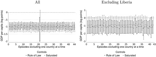
Robustness check for low- and middle-income countries. Note: Dots indicate estimated coefficients. The bars indicate a 90% confidence interval.
Source: Author’s elaboration based on data as presented in Section 3.
The same exercise is performed for the sample of high-income countries. As shown in Figure 2, Hong Kong is an outlier, decreasing the positive aggregated coefficient’s size and statistical significance. Excluding that economy, the positive impact of FDI stock in the long-run economic growth of rich economies becomes larger and highly significant.
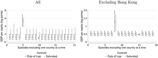
Robustness check for high-income countries. Note: Dots indicate estimated coefficients. The bars indicate a 90% confidence interval.
Source: Author’s elaboration based on data as presented in Section 3.
Overall, these results, combined with the use of different controls in the previous subsections, suggest that the stylized facts identified above—a negative relationship between foreign capital and long-run economic growth in the case of low- and middle-income countries and a positive one for high-income ones—are significantly robust. I also test the robustness of the results on the group of other variables (exports composition, etc.) of the exclusion of these outliers; as can be seen in the appendix (Tables C1 and C2), in both cases, the results persist, and in the case of high-income countries, become even more significant (statistically and in terms of economic meaning).
5. Discussion and concluding remarks
The idea that capital ownership might be important for economic development has been in a long trend of discredit. On theoretical grounds, the canonical policy recommendations stemming from the more widely accepted economic theories would allow capital to circulate freely and open the economies to international trade. This would allow factors’ remuneration to equalize and economies to explore their comparative advantages, increasing aggregate production. This shift has also been met by political changes, such as the shift towards liberalism in the West, the fall of an alternative capital ownership arrangement represented by the Soviet Union, and, finally, the advance of globalization.17 In developing countries, which are relatively scarce in capital, this general view was translated into a common sense that foreign capital is essential to economic development, not only because these economies need capital in ‘quantitative’ terms but also due to the belief that foreign capital would be qualitatively different by incorporating higher technology. The main assumption is, then, that this technology embedded in the foreign capital would spill over to the various sectors of the host economy and increase its productivity.
The theoretical and empirical evidence presented in Section 2 indicates that foreign capital entrance tends to positively affect the host economy in specific circumstances, particularly if the incumbents’ firms in the latter have the tools to react to such entrance. That is, an MNC’s entrance behaves as a competitive shock, and if the established companies can compete with it by increasing their productivity, the whole economy tends to benefit, at least in the short run. In less developed countries, where indigenous firms have worse conditions to compete, the idea that technological upgrading will happen is, thus, questionable. This might occur in economies with very low levels of development, as Meyer and Sinani (2009) point out, given that basic improvements can be accomplished by the mere presence of a multinational company in a region. However, for middle-income countries, whose technological upgrading relies on more active use of ‘absorptive capabilities’, the idea that technology will spill over from the foreign company to the rest of the economy seems questionable. Moreover, the ‘competitive shock’ represented by a multinational firm is specific to a sector and has, thus, heterogeneous effects on the economy, both statically and over time.
Some firm-level empirical evidence indicates a productivity increase after the entrance of foreign firms in a given country. This, however, should not be confused with knowledge spillover and technological upgrading. The productivity gains, in the case of underdeveloped countries, seem to stem from (i) local firms focussing on the production of those commodities that are relatively more efficient and (ii) larger and more efficient production of non-specialized inputs demanded by the MNC. In both cases, the positive effect on productivity is apparent; however, they also have in common another aspect: they reinforce the country’s specialization on its static comparative advantage. And, thus, its potential negative dynamic effects on the host country’s development should also be clear. By constraining indigenous firms to produce less complex goods, innovation production and dissemination18 would be reduced, as well as demand for skilled labour, which also affects its supply over time, as the evidence of path-dependency presented by Te Velde and Xenogiani (2007) indicates.
Using a sample of 44 economies classified as having low or middle-income in 1980, I find robust evidence that a larger stock of foreign capital is associated, in these developing economies, with lower accumulated GDP growth over almost 40 years. Moreover, a larger stock of foreign direct investment is associated with a larger share of low-tech goods in the export basket, which also tends to be less specialized and with a lower level of complexity.
It is possible to interpret these results in light of the large FDI literature as evidence of the necessity of pre-conditions in the host economy for positive effects of foreign capital and of the predominance of vertical knowledge transfers and backward pecuniary externalities given that MNCs tend to produce final goods when in developing economies. These effects tend to have a positive impact in the short run but might generate detrimental dynamic consequences, with local manufacturers specializing in producing inputs whose productivity gains might be transferred to the MNCs via lower prices due to the monopsonistic power of these firms. These results are robust to a number of controls often adopted in the literature to explain long-run growth, such as institutional quality, cost of investment and geographical distribution.
The article also presents some evidence supporting the idea that foreign capital can be positive for more developed economies. In those countries, higher initial levels of foreign capital stock tended to be related to a more specialized basket of exports, which is also less concentrated on low-tech goods.
A number of improvements and extensions are important to consolidate the results and better understand its channels; to start with, an alternative and complete measure of foreign capital stock and a deeper investigation of the lack of specialization of exports in developing economies with larger foreign capital. The goal of this article is to retake an idea that has a long history by presenting theoretical, econometric and historical evidence: capital nationality matters for long-run economic development. The entrance of foreign firms tends to be positive in some circumstances, as indicated. However, the transition from middle levels of development into high ones requires production based on knowledge-based assets, which are firm-specific. A predominance of foreign firms at this intermediate level of development can crowd out indigenous firms in those industries, reducing domestic income via lower profits (no technological rents) and wages (lower overall productivity and persistence of duality in the labour market), and precluding the endogenous growth of such knowledge-based assets, reinforcing static comparative advantages.
I would like to express my gratitude for the comments and suggestions provided by Peter Skott, Arslan Razmi, Daniele Girardi, Christian Rojas, Laura Carvalho and the anonymous referees.
Conflict of interest statement. None declared.
Bibliography
Footnotes
As referred by Lavoie (2022).
These examples of pecuniary spillovers are positive; however, as might be clear, this need not be the case. If the MNC behave as an enclave and imports most of its inputs, for example, the demand for local inputs can be reduced, which, following the same reasoning used to argue for positive leakages, tends to increase input prices and decrease their variety, affecting negatively also other firms and sectors.
These effects seem to assume that (i) resources are binding, which might be the case more for capital than for labour in underdeveloped countries; and (ii) that the MNC and local firms produce substitutable goods.
Another literature for which FDI flows can have an important effect on economic growth is Balance of Payments Constrained Growth Models. Since the seminal contribution by Thirlwall (1979), a number of extensions and empirical tests have been made on the matter; the basic idea is that given different elasticities to import and export, developing countries would tend to have their income growth limited by the availability of foreign currency. Within this framework, an increase in FDI can relax this constraint and allow for higher domestic growth rates. This channel, however, is linked only by chance to the issue of capital ownership, the core of our argument, as its effect operates just as any other inflow of foreign currency. Therefore, it will not be the focus of this analysis.
For instance, Alfaro et al. (2010) present a model in which this channel is explicit. In it, final goods are produced by combining intermediate goods that can be either domestic or foreign; these intermediate goods are produced in a competitive market using skilled and unskilled labour and a range of differentiated inputs. These differentiated inputs (a second upstream industry layer) are produced in a monopolistic competition environment. To operate in the intermediate input sector, one must develop a new variety of intermediate inputs, which requires upfront capital—and this is where financial markets can be crucial. In the model language, the increase in the varieties of intermediate inputs encouraged by the MNC entrance and allowed by a sufficiently developed local market leads to positive backward and forward leakages.
The presence of non-linearities also appears in Jude and Levieuge (2017), in which the authors find that for an ‘institutional index’, there is a threshold below which FDI has no positive effect.
This conciliatory explanation is also found in Harrison and Rodriguez-Clare (2010), for instance.
The threshold, equivalent to a male population above 25 years with 0.52 years of secondary schooling on average, was satisfied by 46 out of 69 countries in the authors’ sample. When the authors test the level of human capital needed for foreign investment to have a larger effect on growth than domestic investment, the threshold becomes stricter, with only 29 countries meeting it.
As pointed out by the authors, one can argue that, in terms of Kosova (2010), this captures only the static net effect.
Besides these incentives to the private sector, government direct intervention, particularly in infrastructure investment, was important to increase physical capital and ensure demand for the emerging sectors.
According to Amsden (2001), in industry segments with low entry costs (e.g. processing of imported inputs in pharmaceuticals or certain forms of electronic assembly), MNCs did not constitute an entry barrier to local firms and probably involved some knowledge transfer. However, the most important high-tech sectors have high sunk costs, so the first-mover advantage is high, and firms initially established tend to crowd out other enterprises in the future. This would be important historically because Latin America was one of the first regions to receive multinationals in those sectors, given its proximity with the USA and its type of industrialization, labelled as emigre type—initiated by migrants from developed countries and later by multinational firms. In other countries that developed faster after 1960, the industrialization experience was related to colonization. This would have ended up being an advantage given that the decolonization process enabled them to stay with their productive structure but without foreign ownership. This process would have happened in different forms in China, India, Korea and Taiwan, for instance—all countries that managed to grow fast after the second World War, resume growth after the 1990s crises, and move to a higher technological productive structure.
It is not claimed, therefore, that an increase in the stock of FDI as a share of GDP represents an increase in the stock of capital of the host country, but only that a larger share of the existing capital is owned by a non-resident.
See, for instance, Globerman and Shapiro (2002), Daude and Stein (2007) and Méon and Sekkat (2004).
On the growth literature, geography is explored as a factor of growth as it might be related to aspects such as climate (affecting agricultural productivity and health, for instance) and transportation costs. See, for instance, Rodrik (2003).
The results indicate that countries that start with one log(GDP) per capita higher will have a −0.30 lower accumulated log GDP per capita; as an illustration, a country with a GDP per capita 50% higher will have a 7.7% smaller accumulated GDP per capita. The interpretation of coefficients of indexes, such as the rule of law and income Gini, is less illustrative.
Given that our main interest is the effect of foreign capital stock, I omit the coefficients of other variables.
In recent years, there have been some indications of a retreat in free trade ideology, as evidenced by an increase in tariffs in the USA and more explicit discussions about industrial policy. These, so far, however, are still short-term fluctuations when compared to the general trend towards globalization.
As mentioned, it is likely that some improvement related to better technology reaches backward sectors, but it tends to be contained there, and most of its gains are absorbed by the MNC.
Appendices
A List of countries
List of low- and middle-income countries
| Country | Foreign K (%GDP) | Growth | Country | Foreign K (%GDP) | Growth |
|---|---|---|---|---|---|
| Algeria | 3.61 | 25.5% | Mali | 12.31 | 196.6% |
| Angola | 0.85 | 2.7% | Morocco | 10.33 | 91.7% |
| Argentina | 2.55 | 19.5% | Mozambique | 0.23 | 84.0% |
| Bangladesh | 2.76 | 128.0% | Niger | 5.29 | −25.0% |
| Bolivia | 11.93 | 45.1% | Nigeria | 1.01 | 27.9% |
| Brazil | 9.15 | 26.0% | Pakistan | 2.23 | 77.1% |
| Cambodia | 5.28 | 167.6% | Paraguay | 3.91 | 51.4% |
| Chile | 35.31 | 107.5% | Peru | 5.35 | 56.5% |
| China | 0.35 | 207.3% | Philippines | 3.56 | 62.6% |
| Colombia | 2.26 | 68.6% | Portugal | 9.34 | 69.2% |
| Congo | 17.06 | −4.8% | Republic of Korea | 1.74 | 206.1% |
| Côte d’Ivoire | 5.21 | 25.0% | Senegal | 3.56 | 38.0% |
| Egypt | 11.24 | 114.5% | South Africa | 19.62 | 8.9% |
| El Salvador | 13.11 | 48.7% | Sri Lanka | 4.71 | 151.6% |
| India | 0.24 | 162.7% | Thailand | 2.92 | 154.5% |
| Indonesia | 5.38 | 139.6% | Tunisia | 34.80 | 77.5% |
| Iran | 3.10 | 24.5% | Turkey | 9.29 | 111.0% |
| Jamaica | 16.98 | 21.3% | Uganda | 0.34 | 100.3% |
| Kenya | 3.67 | 35.2% | Uruguay | 3.97 | 70.7% |
| Lebanon | 0.37 | 4.6% | Venezuela | 2.32 | −105.5% |
| Liberia | 92.86 | −60.8% | Zambia | 46.30 | 25.2% |
| Malaysia | 21.11 | 131.6% | Zimbabwe | 2.26 | 47.2% |
Source: Author’s elaboration based on data as presented in Section 3.
List of high-income countries
| Country | Foreign K (%GDP) | Growth | Country | Foreign K (%GDP) | Growth |
|---|---|---|---|---|---|
| Australia | 14.30 | 61.18 | Italy | 1.86 | 37.03 |
| Austria | 3.85 | 60.46 | Japan | 0.30 | 64.75 |
| Belgium | 5.76 | 56.09 | Netherlands | 12.43 | 61.99 |
| Canada | 19.62 | 48.82 | New Zealand | 10.12 | 59.50 |
| Hong Kong | 615.88 | 123.33 | Norway | 10.24 | 64.05 |
| Denmark | 5.90 | 60.12 | Singapore | 44.29 | 145.10 |
| Finland | 0.85 | 66.04 | Spain | 2.21 | 66.02 |
| France | 4.51 | 49.57 | Sweden | 2.01 | 64.16 |
| Greece | 7.96 | 23.55 | UK | 11.15 | 67.95 |
| Ireland | 162.95 | 151.56 | USA | 2.89 | 67.79 |
| Israel | 13.21 | 75.78 |
Source: Author’s elaboration based on data as presented in Section 3.
Testing endogeneity of FDI stock in 1980
| Dependent variable: accumulated GDP per capita growth (1980–1970) | ||
|---|---|---|
| Low- and middle-income countries | High-income countries | |
| Foreign Capital Stock (1980) | −0.07 | 0.06 |
| (0.32) | (0.17) | |
| Dependent variable: accumulated GDP per capita growth (1980–1970) | ||
|---|---|---|
| Low- and middle-income countries | High-income countries | |
| Foreign Capital Stock (1980) | −0.07 | 0.06 |
| (0.32) | (0.17) | |
Note: Robust (Clustered) standard errors are in parentheses.
**indicates statistical significance at 10%,
* at 5%.
Source: Author’s elaboration based on data as presented in Section 3.
B Using five years average
OLS regressions—other variables—five years average—low- and middle-income countries
| (1) | (2) | (3) | (4) | (5) | (6) | |
|---|---|---|---|---|---|---|
| Human Capital | 0.02 | 0.01 | −0.00 | 0.01 | −0.00 | 0.01 |
| (0.04) | (0.04) | (0.05) | (0.05) | (0.04) | (0.05) | |
| Agr (% GDP) | 3.21 | 1.58 | 2.51 | 0.02 | 1.13 | 4.68* |
| (2.22) | (1.52) | (1.70) | (1.04) | (1.54) | (1.94) | |
| Man (% GDP) | −1.83** | −1.53 | −0.33 | −1.20 | 0.01 | 0.77 |
| (1.02) | (1.14) | (0.97) | (0.89) | (1.07) | (0.95) | |
| Serv (% GDP) | −0.43 | −0.28 | −0.06 | 0.04 | 0.07 | 0.01 |
| (0.37) | (0.31) | (0.28) | (0.22) | (0.23) | (0.35) | |
| EXPY | −0.75* | −0.64* | −0.68 | −0.77* | −0.62** | −1.09** |
| (0.33) | (0.31) | (0.27) | (0.36) | (0.32) | (0.62) | |
| Gini (X) | −0.19** | −0.20* | −0.19* | −0.27* | −0.15 | −0.31* |
| (0.10) | (0.09) | (0.09) | (0.09) | (0.11) | (0.10) | |
| Theil (X) | −1.09 | −1.13** | −1.13** | −1.61* | −0.92 | −1.97* |
| (0.63) | (0.64) | (0.57) | (0.64) | (0.76) | (0.62) | |
| HHI (X) | −8.25 | −7.64 | −7.56 | −8.56 | −5.80 | −12.15** |
| (4.99) | (5.05) | (4.49) | (5.14) | (5.44) | (6.45) | |
| Share high-tech (X) | 1.84 | 2.54 | 2.31 | 2.57 | 3.19 | 1.90 |
| (1.57) | (2.06) | (2.06) | (2.33) | (2.82) | (1.71) | |
| Share Commodities (X) | −1.05 | −2.20 | −0.92 | −2.01 | −2.94 | −5.66 |
| (4.19) | (3.42) | (3.62) | (3.21) | (2.62) | (3.79) | |
| Share low-tech (X) | 4.67* | 3.54* | 3.23* | 2.10* | 1.78** | 3.50* |
| (2.17) | (1.48) | (1.53) | (1.00) | (1.01) | (1.58) | |
| TFP | −0.06 | 0.16 | −0.40 | 0.19 | −0.20 | −0.53 |
| (0.49) | (0.32) | (0.38) | (0.40) | (0.38) | (0.57) |
Notes: Coefficients for the independent variable of interest (stock of foreign capital as a share of GDP—average from 1980 to 1985) on the dependent variable given in each line. Column (1) controls for the rule of law index; column (2) controls for initial GDP; column (3) for the share of commodities on exports; column (4) controls for initial income inequality; column (5) controls for the share of low-tech manufactures on exports; and column (6) controls for initial GDP, rule of law, the share of commodities on exports, the share of low-tech goods on exports, and income inequality. Robust standard errors are in parentheses.
**indicates statistical significance at 10%,
*at 5%.
Source: Author’s elaboration based on data as presented in Section 3.
OLS regressions—five years average—low- and middle-income countries
| (1) | (2) | (3) | (4) | (5) | (6) | (7) | (8) | (9) | |
|---|---|---|---|---|---|---|---|---|---|
| Dependent variable: GDP per capita growth (2019–1980) | |||||||||
| Foreign Capital Stock | −0.78* | −0.81* | −0.94* | −0.74* | −0.76* | −0.58* | −0.73** | −0.58** | −1.06* |
| (0.32) | (0.23) | (0.16) | (0.23) | (0.31) | (0.22) | (0.37) | (0.32) | (0.17) | |
| Initial GDP per capita | −14.53 | −31.06* | |||||||
| (11.06) | (14.71) | ||||||||
| Human Capital | 24.03 (24.32) | ||||||||
| Rule of Law | 41.57* | 76.13* | |||||||
| (11.00) | (17.39) | ||||||||
| Latitude | 87.61 (64.27) | ||||||||
| Price of Investment | −61.80** (31.33) | ||||||||
| Share Commodities X | −1.07* | 0.84 | |||||||
| (0.43) | (0.74) | ||||||||
| Income Inequality | −226.83* | −85.11 | |||||||
| (100.52) | (100.03) | ||||||||
| Share low-tech X | 1.39* | 0.65 | |||||||
| (0.56) | (0.87) | ||||||||
Notes: All variables are their average levels from 1980 to 1985, except for the rule of law variable, which continues to be a five-year average of the index from 2010 to 2015. The latitude is given by an index from 0 to 1. Share Commodities X is the share of commodities in the export basket. Income inequality is measured as the pre-tax Gini index. Robust standard errors are in parentheses.
**indicates statistical significance at 10%,
at 5%.
Source: Author’s elaboration based on data as presented in Section 3.
OLS regressions—other variables—five years average—high-income countries
| (1) | (2) | (3) | (4) | (5) | (6) | |
|---|---|---|---|---|---|---|
| Human Capital | 0.02* | 0.00 | 0.01* | 0.02* | 0.01 | 0.04 |
| (0.00) | (0.01) | (0.00) | (0.01) | (0.01) | (0.03) | |
| Agr (% GDP) | −80.59* | −74.66* | −81.66* | −79.70* | −89.63* | −67.04** |
| (8.38) | (7.52) | (3.59) | (10.46) | (6.79) | (22.19) | |
| Man (% GDP) | 0.47 | 0.66 | 0.56** | 1.10 | 1.36* | 2.72** |
| (0.43) | (0.78) | (0.27) | (0.78) | (0.44) | (0.67) | |
| Serv (% GDP) | −0.05 | −0.11* | −0.02 | −0.09 | 0.01 | −0.12 |
| (0.04) | (0.03) | (0.04) | (0.05) | (0.06) | (0.27) | |
| EXPY | 0.02 | 0.00 | 0.02 | 0.01 | 0.02 | 0.03 |
| (0.01) | (0.01) | (0.01) | (0.01) | (0.02) | (0.03) | |
| Gini (X) | 0.01* | 0.01* | 0.01* | 0.01* | 0.02* | 0.03** |
| (0.00) | (0.01) | (0.00) | (0.00) | (0.01) | (0.01) | |
| Theil (X) | 0.03** | 0.04** | 0.03** | 0.03 | 0.06* | 0.07 |
| (0.02) | (0.02) | (0.02) | (0.02) | (0.03) | (0.05) | |
| HHI (X) | 0.08* | 0.07 | 0.08* | 0.06 | 0.11* | 0.14 |
| (0.04) | (0.05) | (0.04) | (0.04) | (0.05) | (0.12) | |
| Share high-tech (X) | 0.05* | 0.01 | 0.05* | 0.04** | 0.01 | −0.05 |
| (0.01) | (0.03) | (0.01) | (0.02) | (0.04) | (0.06) | |
| Share Commodities (X) | −0.27 | 0.17 | −0.24 | −0.14 | −0.66 | −0.97 |
| (0.21) | (0.35) | (0.22) | (0.23) | (0.42) | (0.80) | |
| Share low-tech (X) | −0.29* | −0.11 | −0.28* | −0.21* | −0.17* | 0.02 |
| (0.03) | (0.09) | (0.03) | (0.06) | (0.08) | (0.14) | |
| TFP | 0.03* | 0.05* | 0.03** | 0.04* | 0.07* | 0.05 |
| (0.01) | (0.02) | (0.02) | (0.02) | (0.03) | (0.04) |
Notes: Coefficients for the independent variable of interest (stock of foreign capital as a share of GDP—average from 1980 to 1985) on the dependent variable given in each line. Column (1) controls for the rule of law index; column (2) controls for initial GDP; column (3) for the share of commodities on exports; column (4) controls for initial income inequality; column (5) controls for the share of low-tech manufactures on exports; and column (6), controls for initial GDP, rule of law, the share of commodities on exports, the share of low-tech goods on exports, and income inequality. Robust standard errors are in parentheses.
**indicates statistical significance at 10%,
*at 5%.
Source: Author’s elaboration based on data as presented in Section 3.
OLS regressions—five years average—high-income countries
| (1) | (2) | (3) | (4) | (5) | (6) | (7) | (8) | (9) | |
|---|---|---|---|---|---|---|---|---|---|
| Dependent variable: GDP per capita growth (2019–1980) | |||||||||
| Foreign Capital Stock | 0.11* | 0.12* | 0.13* | 0.11** | 0.13* | 0.13* | 0.13* | 0.20* | 0.21* |
| (0.05) | (0.05) | (0.04) | (0.06) | (0.04) | (0.04) | (0.05) | (0.05) | (0.08) | |
| Initial GDP per capita | −20.92 | −65.03 | |||||||
| (25.82) | (37.06) | ||||||||
| Human Capital | −15.20 (21.24) | ||||||||
| Rule of Law | 17.70* | −0.68 | |||||||
| (7.39) | (16.63) | ||||||||
| Latitude | −43.33 (51.64) | ||||||||
| Price of Investment | −75.89 (115.73) | ||||||||
| Share Commodities X | −0.04 | −0.54* | |||||||
| (0.12) | (0.25) | ||||||||
| Income Inequality | −1.95 | −108.22 | |||||||
| (64.41) | (110.30) | ||||||||
| Share low-tech X | −1.20* | −2.29** | |||||||
| (0.56) | (1.28) | ||||||||
Notes: All variables are their average levels from 1980 to 1985, except for the rule of law variable, which continues to be a five-year average of the index from 2010 to 2015. The latitude is given by an index from 0 to 1. Share Commodities X is the share of commodities in the export basket. Income inequality is measured as the pre-tax Gini index. Robust standard errors are in parentheses.
**indicates statistical significance at 10%,
*at 5%.
Source: Author’s elaboration based on data as presented in Section 3.
C Results for other variables excluding outliers
Low- and middle-income countries—excluding Liberia
| (1) | (2) | (3) | (4) | (5) | (6) | |
|---|---|---|---|---|---|---|
| Human Capital | 0.11 | 0.04 | 0.06 | 0.10 | 0.09 | 0.21 |
| (0.13) | (0.14) | (0.21) | (0.14) | (0.20) | (0.22) | |
| Agr (% GDP) | 2.77 | 1.23 | 0.12 | −0.62 | −1.56 | 2.37 |
| (2.06) | (1.51) | (2.44) | (1.12) | (2.43) | (3.15) | |
| Man (% GDP) | −2.66* | −2.05 | −0.54 | −1.67 | −0.36 | 0.66 |
| (1.23) | (1.40) | (1.11) | (1.15) | (1.16) | (1.22) | |
| Serv (% GDP) | −0.78 | −0.33 | −0.11 | 0.11 | 0.13 | −0.19 |
| (0.63) | (0.48) | (0.46) | (0.38) | (0.31) | (0.58) | |
| EXPY | −0.81** | −0.64 | −0.78** | −0.89** | −0.72 | −0.90 |
| (0.47) | (0.45) | (0.42) | (0.47) | (0.43) | (0.73) | |
| Gini (X) | −0.15 | −0.21* | −0.17* | −0.19* | −0.15 | −0.13 |
| (0.11) | (0.09) | (0.08) | (0.09) | (0.09) | (0.12) | |
| Theil (X) | −1.00 | −1.24* | −1.13* | −1.17** | −0.97 | −0.77 |
| (0.62) | (0.56) | (0.50) | (0.59) | (0.64) | (0.73) | |
| HHI (X) | −7.13** | −7.01** | −6.89** | −7.42** | −5.95 | −8.15 |
| (3.99) | (3.97) | (3.44) | (4.13) | (4.34) | (4.91) | |
| Share high-tech (X) | 1.95 | 3.07 | 2.99 | 3.24 | 3.39 | 1.82 |
| (1.46) | (1.97) | (1.88) | (1.95) | (2.23) | (1.42) | |
| Share Commodities (X) | 1.69 | 0.11 | 0.44 | −0.44 | −1.68 | −0.65 |
| (4.48) | (3.45) | (3.59) | (3.18) | (2.77) | (4.64) | |
| Share low-tech (X) | 4.96* | 4.24* | 3.72* | 2.78** | 2.64** | 3.82** |
| (2.43) | (1.67) | (1.75) | (1.40) | (1.40) | (1.97) | |
| TFP | 0.00 | 0.24 | −0.51 | 0.23 | −0.32 | −0.50 |
| (0.61) | (0.40) | (0.43) | (0.49) | (0.38) | (0.55) |
Notes: Coefficients for the independent variable of interest, stock of foreign capital as a share of GDP. Column (1) controls for the rule of law index; column (2) controls for initial GDP; column (3) for the share of commodities on exports; column (4) controls for initial income inequality; column (5) controls for the share of low-tech manufactures on exports; and column (6), controls for initial GDP, rule of law, the share of commodities on exports, the share of low-tech goods on exports, and income inequality. Robust standard errors are in parentheses.
**indicates statistical significance at 10%,
*at 5%.
Source: Author’s elaboration based on data as presented in Section 3.
High-income countries—excluding Hong Kong
| (1) | (2) | (3) | (4) | (5) | (6) | |
|---|---|---|---|---|---|---|
| Human Capital | 0.05 | 0.00 | 0.05 | 0.03 | 0.04 | 0.03 |
| (0.06) | (0.05) | (0.07) | (0.06) | (0.07) | (0.06) | |
| Agr (% GDP) | −96.30* | −86.86* | −100.83* | −96.60* | −109.71* | −90.24* |
| (11.69) | (11.77) | (4.73) | (15.01) | (9.57) | (12.66) | |
| Man (% GDP) | 0.13 | 0.31 | 0.43 | 0.82 | 1.32* | 2.17* |
| (0.52) | (0.93) | (0.28) | (0.78) | (0.38) | (0.29) | |
| Serv (% GDP) | −0.07 | −0.26* | 0.00 | −0.13 | 0.10 | −0.20 |
| (0.09) | (0.07) | (0.06) | (0.11) | (0.11) | (0.17) | |
| EXPY | 0.17* | 0.14* | 0.16* | 0.16* | 0.16* | 0.16* |
| (0.04) | (0.03) | (0.04) | (0.03) | (0.04) | (0.04) | |
| Gini (X) | 0.05* | 0.07* | 0.06* | 0.06* | 0.05* | 0.08* |
| (0.01) | (0.01) | (0.01) | (0.01) | (0.01) | (0.02) | |
| Theil (X) | 0.19* | 0.23* | 0.19* | 0.20* | 0.19* | 0.25* |
| (0.04) | (0.05) | (0.03) | (0.03) | (0.03) | (0.06) | |
| HHI (X) | 0.42* | 0.47* | 0.39* | 0.43* | 0.40* | 0.46* |
| (0.14) | (0.16) | (0.12) | (0.12) | (0.10) | (0.19) | |
| Share high-tech (X) | 0.13* | 0.05 | 0.12** | 0.11* | 0.14** | 0.07 |
| (0.06) | (0.07) | (0.06) | (0.05) | (0.08) | (0.10) | |
| Share Commodities (X) | −3.57 | −2.64 | −3.71 | −3.54 | −3.38 | −2.36 |
| (2.35) | (1.91) | (2.51) | (2.27) | (2.13) | (1.68) | |
| Share low-tech (X) | −0.43* | −0.16 | −0.35* | −0.36* | −0.40* | −0.21 |
| (0.10) | (0.19) | (0.12) | (0.13) | (0.10) | (0.29) | |
| TFP | 0.11* | 0.17* | 0.15* | 0.15* | 0.13* | 0.14* |
| (0.04) | (0.05) | (0.04) | (0.04) | (0.05) | (0.05) |
Notes: Coefficients for the independent variable of interest, stock of foreign capital as a share of GDP. Column (1) controls for the rule of law index; column (2) controls for initial GDP; column (3) for the share of commodities on exports; column (4) controls for initial income inequality; column (5) controls for the share of low-tech manufactures on exports; and column (6), controls for initial GDP, rule of law, the share of commodities on exports, the share of low-tech goods on exports, and income inequality. Robust standard errors are in parentheses.
**indicates statistical significance at 10%,
*at 5%.
Source: Author’s elaboration based on data as presented in Section 3.
