


Abstract
Brain energy budgets specify metabolic costs emerging from underlying mechanisms of cellular and synaptic activities. While current bottom–up energy budgets use prototypical values of cellular density and synaptic density, predicting metabolism from a person’s individualized neuropil density would be ideal. We hypothesize that in vivo neuropil density can be derived from magnetic resonance imaging (MRI) data, consisting of longitudinal relaxation (T1) MRI for gray/white matter distinction and diffusion MRI for tissue cellularity (apparent diffusion coefficient, ADC) and axon directionality (fractional anisotropy, FA). We present a machine learning algorithm that predicts neuropil density from in vivo MRI scans, where ex vivo Merker staining and in vivo synaptic vesicle glycoprotein 2A Positron Emission Tomography (SV2A-PET) images were reference standards for cellular and synaptic density, respectively. We used Gaussian-smoothed T1/ADC/FA data from 10 healthy subjects to train an artificial neural network, subsequently used to predict cellular and synaptic density for 54 test subjects. While excellent histogram overlaps were observed both for synaptic density (0.93) and cellular density (0.85) maps across all subjects, the lower spatial correlations both for synaptic density (0.89) and cellular density (0.58) maps are suggestive of individualized predictions. This proof-of-concept artificial neural network may pave the way for individualized energy atlas prediction, enabling microscopic interpretations of functional neuroimaging data.
Introduction
Functional imaging methods like functional magnetic resonance imaging (fMRI) and positron emission tomography (PET) enable noninvasive imaging of metabolism in the human brain as proxies for electrical activity (Hyder and Rothman 2017). Specifically, glucose oxidation (CMRglc(ox)) is dynamically related to changes in neuronal activity (Smith et al. 2002; Maandag et al. 2007). Such noninvasive yet volumetric modalities are very powerful tools for imaging brain activity across mental states and disease (Mortensen et al. 2018), and have yielded much progress in our understanding regarding the metabolic basis of human brain function (Shulman et al. 2009, 2014). The brain’s cognitive capabilities, however, is result of the intricate interplay between structure and function (Yu et al. 2018), and the metabolic imaging we take for granted is based on neuropil density which encompasses both cellular and synaptic interactions. Understanding neuronal and synaptic circuits is key to modeling and deciphering the metabolic features underlying cortical functions in health and disease (Laughlin and Sejnowski 2003; Wolf et al. 2014; Yu et al. 2023).
A more direct measure of cognitive activity would measure neural electrical activity or neural firing rate instead of metabolism. Such information can be acquired noninvasively through scalp electroencephalography (EEG), but the presence of skull and intervening tissues between the brain and EEG electrodes reduces spatial resolution and introduces signal source localization ambiguity (Ferree et al. 2001; Wendel et al. 2009). Additionally, EEG is differentially sensitive to superficial layers of the brain, and to different sources of neuropil electrical activity (Kirschstein and Kohling 2009). Magnetoencephalography (MEG) is a similar noninvasive imaging modality, which maps electrical currents by detecting the associated magnetic fields. However, localization for MEG is also difficult and imprecise, with no exact inverse solution for reconstructing the exact location and magnitude of brain currents (Cohen et al. 1990; Wendel et al. 2009). EEG and MEG do, however, have distinct and complimentary sensitivities enabling more accurate source localization when used in tandem (Sharon et al. 2007). While EEG can be configured with functional imaging methods like fMRI and PET, coalescence of MEG and fMRI or PET may be far more challenging.
Adenosine triphosphate (ATP), the currency of cellular energy, is produced by oxidizing glucose (or CMRglc(ox)), where glucose is the main sugar utilized by the brain. Since the brain has no glucose and oxygen reserves, the brain must import these nutrients from the blood according to local demand. Metabolic imaging modalities like calibrated fMRI and PET measure glucose and oxygen metabolism in vivo as a proxy for brain activity. The metabolic cost of electrical activity at the neuropil involves several processes (e.g. maintenance and restoration of resting membrane potential, generation and propagation of action potentials and synaptic transmission, recycling of neurotransmitters, and housekeeping needs) which collectively comprise an “energy budget” (Attwell and Laughlin 2001; Yu et al. 2018). Modeling brain energetics via the energy budget can potentially extract microscopic information on electrical activity from metabolic imaging, which can then be related to EEG or MEG measurements of human subjects.
Bottom–up energy budgets aim to comprehensively model the brain’s metabolic demands, which depends on the brain’s level of electrical activity and cellular energetics of the underlying neuropil anatomy. This inherently necessitates that bottom–up energy budgets require a certain level of understanding of cellular and synaptic densities. By explicitly modeling the relationships between these aspects of brain function, it becomes possible to use energetic and anatomical measurements to quantify electrical activity throughout the brain (Fig. 1), or to predict the metabolic consequences of different perturbations such as a reduction in cellular (CellDen) or synaptic (SynDen) density.
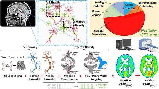
Schematic on how to build a brain energy atlas based on neuropil density, which is comprised of cellular (CellDen) and synaptic (SynDen) density (Yu et al. 2023). The brain’s CMRglc(ox) is based on various energy budget components like housekeeping needs, resting potential and action potential, synaptic transmission, neurotransmitter recycling, and calcium–ion-related costs (Yu et al. 2023). Each of these components are scaled differentially with CellDen and SynDen, and then active terms scale by firing rates. Summing all energy budget components provides the computed or in silico CMRglc(ox). By comparing these to the measured or in vivo CMRglc(ox) novel microscopic insights into the basis of brain’s metabolic heterogeneity can be gained. Our recent study on brain energy atlas based on neuropil density (Yu et al. 2023) used BigBrain, an ex vivo histology for CellDen (Amunts et al. 2013) and in vivo PET imaging of SynDen (Finnema et al. 2016). The goal of this study is to create individualized neuropil density (i.e. CellDen and SynDen on each person) such that personalized in silico CMRglc(ox) can be created and then compared with their own in vivo CMRglc(ox) as measured by calibrated fMRI (Chen et al. 2022).
Neuropil density is fundamental for such metabolic modeling as it represents the infrastructure necessary for function. Prior bottom–up energy budgets utilized generalized neuropil density representing prototypical measures of CellDen and SynDen to model the brain’s energetic metabolism as a whole, without considering how these densities may vary across various cortical and subcortical regions. Our recent advance in spatially resolved human brain energy budgets, or energy atlas (Yu et al. 2023), was based on CellDen acquired ex vivo from a single 65-year-old healthy subject (Amunts et al. 2013) and an in vivo PET-measured SynDen atlas created from a group of young healthy subjects (Finnema et al. 2016). The energy atlas calculation of CMRglc(ox) (Yu et al. 2023) was validated by PET-measured CMRglc(ox) (Hyder et al. 2016) to reveal, for the first time, heterogeneous neuronal activity rates averaging around 1.2 Hz globally for the cerebral cortex (Yu et al. 2023). To noninvasively image electrical activity, a major innovation in energy budget modeling will be to predict metabolism from personalized neuroanatomy.
Various methods have been developed to probe the brain’s anatomy. They range from ex vivo histology (Amunts et al. 2013) to isotropic fractionation to acquire cell counts for different brain tissues but devoid of spatial information (Herculano-Houzel and Lent 2005), to approaches for in vivo measurement with PET imaging for synaptic density (Finnema et al. 2016). However, an efficient and effective means of in vivo measurement of neuropil density is still needed. Here we present an approach using machine learning to measure neuropil density (i.e. both CellDen and SynDen) from in vivo MRI data. To reflect gray/white matter (GM/WM) tissue we used MRI weighted by longitudinal relaxation (T1) using magnetization-prepared 180o radio-frequency pulses and rapid gradient-echo (MPRAGE). To depict tissue cellularity and axon directionality, we used diffusion-weighted imaging (DWI) with apparent diffusion coefficient (ADC) and fractional anisotropy (FA). Our algorithm used T1/ADC/FA on a nonspatial, voxel-by-voxel basis to predict CellDen and SynDen maps by training and comparing neuropil density predictions from MRI on several subjects to our reference standards of ex vivo histology (Amunts et al. 2013) for CellDen and in vivo PET imaging (Finnema et al. 2016) for SynDen. This first proof-of-concept feasibility study shows that with in vivo MRI data on a subject basis we can potentially estimate individualized neuropil densities, and by extension, individualized energy atlases.
Materials and methods
Anatomical and metabolic datasets
We used MPRAGE, FA, and ADC data from the Alzheimer’s Disease Neuroimaging Initiative (ADNI), a multicenter longitudinal study focused on Alzheimer’s disease, with more information online at adni.loni.usc.edu. We limited subjects to those that were scanned using the ADNI 3 protocol, the latest scanning protocol in the ADNI project. Analysis was further limited to those subjects that were scanned on Siemens 3T scanners for consistency. We selected only the cognitively normal (control) subjects. We further refined our search to those subjects that had both MPRAGE and DWI (both ADC and FA) data available. These search parameters yielded a total of 64 subjects, of whom 10 subjects were randomly selected (Fig. 2a) and the same 10 subjects used for training/validation of all of our networks for this study (with the specific subjects chosen for training and validation among these 10 subjects randomized from network to network), while the remaining 54 subjects were test subjects that were never used to train the networks and were used to test the network predictions.

a). In vivo MRI datasets used to train our ANN machine learning model. Data from 10 healthy control subjects were selected from the ADNI database, with criteria of most recent scanning protocols for 3T Siemens. See Supplementary Table S1 for details. Each column corresponds to a subject and each row represents an MRI contrast in vivo. The top row reflects GM/WM tissue as weighted by T1 using MPRAGE. The second and third rows, respectively, reflect diffusion MRI data for tissue cellularity with ADC and axon directionality with FA. Since MPRAGE provides tissue type information which affects neuropil architecture and the neuropil architecture influences diffusion MRI properties, these MRI datasets and neuropil density are related. We thus hypothesized that such relationships would enable us to predict neuropil density from MPRAGE, ADC, and FA data using machine learning. b) In vivo MRI datasets, averaged over the 10 ADNI subjects in Fig. 2a, with various degrees of spatial smoothing. The 3 rows reflect GM/WM contrast by MPRAGE (top), tissue cellularity by ADC (middle), and axon directionality by FA (bottom). Each column corresponds to different degrees of smoothing (|${\sigma}^3$|), where the leftmost column shows unsmoothed group average data, with successive columns to the right visualizing the data with increasing levels of Gaussian smoothing. Since our ANN model runs on a voxel-by-voxel basis without any data from neighboring voxels, providing several Gaussian-smoothed datasets provides the ANN with neighborhood information. Smoothed datasets provide data that is less noisy and less susceptible to registration errors. Highly smoothed datasets additionally provide subject-wide and specific brain region basis sets for the ANN model (Supplementary Fig. S1) to use for neuropil density predictions. Our final machine learning models for neuropil prediction use the images with white asterisks as inputs, with cubic sigma (|${\sigma}^3$|) values of 0, 1, 8, 64, and 512, and we refer to this as “high-smoothing”. The cubic sigma values of 0, 0.5, 1, 2 and 4 are used instead for some of the “low-smoothing” networks that we present in this study. These values were chosen by examining results from a range of different smoothing levels.
MPRAGE images reflected GM/WM distributions whereas ADC depicted tissue cellularity and FA designated axon directionality. Although based on brain tumor MRI scans (Ginat et al. 2012; Figley et al. 2021), there is a strong negative correlation between ADC vs. GM cellularity and a strong positive correlation between FA vs. WM microstructure. Since MPRAGE provides tissue type information (GM/WM) which affects neuropil architecture which in turn is influencs DWI properties, these MRI datasets and neuropil density are related. We thus hypothesized that such relationships would enable us to predict neuropil density from MPRAGE, ADC, and FA data using machine learning.
In cases where subjects had multiple DWI scans taken, the earliest scans (i.e. when the subjects were youngest) were used. Some of these subjects had multiple T1 MPRAGE scans; those scans taken closest in time to the selected DWI scans were used. Subjects were selected to be unique, so multiple scans, even those taken at different time points/subject ages, were not included for the same subject. The data was available in native space, and the resolution of the ADC and FA datasets from the study was 2 mm isotropic, while the MPRAGE data was at 1.05 × 1.05 × 1.2 mm resolution. Using the FMRIB Software Library (FSL) we affine registered the subjects to Montreal Neurological Institute (MNI) space and resized the data to 3 mm isotropic resolution to match our lowest resolution dataset, which was the PET SynDen data. After these processing steps the MPRAGE, ADC, and FA data from the 10 test/validation subjects or 54 test subjects were also averaged to create test/validation and train group averages respectively.
The goal of this study was to predict the reference standards of CellDen and SynDen from in vivo MRI data. Figure 1 shows an overview of the process involved to create a brain energy atlas which relies on neuropil density which comprises of CellDen and SynDen (Yu et al. 2023). Briefly, CMRglc(ox) has various components which are scaled differentially by CellDen and SynDen, but only the active terms are dependent on firing rates. Microscopic basis of metabolic heterogeneity can be observed by comparing in silico CMRglc(ox) with in vivo CMRglc(ox), e.g. as measured by calibrated fMRI (Chen et al. 2022). Our recent human brain energy atlas (Yu et al. 2023) used BigBrain, an ex vivo histology for CellDen (Amunts et al. 2013) and in vivo PET imaging of SynDen (Finnema et al. 2016). The goal here is to generate individualized neuropil density (i.e. CellDen and SynDen on each person from their own MRI data) by employing machine learning on these datasets such that personalized in silico CMRglc(ox) maps can be created.
Neural network machine learning algorithm
We used an artificial neural network (ANN) machine learning algorithm to predict CellDen and SynDen from MPRAGE, ADC, and FA as shown in Supplementary Fig. S1. Our implementation used MATLAB’s built-in feedforwardnet command. The ANN architecture has 3 hidden layers with 40, 20, and 10 nodes, respectively, with a sigmoid activation function and a linear activation function for the output layer, and was trained to minimize the mean squared error. We trained separate ANNs to predict CellDen and SynDen with no cross training between these networks.
All our ANNs were provided MPRAGE, ADC, and FA (scaled so that the mean value across the cerebrum for each subject image was 0.5) on a voxel-by-voxel basis as input, and predicted CellDen or SynDen one voxel at a time. To provide image neighborhood information, the in vivo MRI datasets were Gaussian-smoothed, with various degrees of smoothing, providing additional inputs to the ANN with neighborhood information. MRI data were smoothed using different Gaussian-smoothing kernels, with 4 different levels of smoothed images for each of MPRAGE, FA, and ADC for any given subject taken and concatenated to form a 15-channel input tensor per voxel prediction (Fig. 2b).
Since individualized CellDen and SynDen data were not available for the different subjects, the same prototypical values (scaled so that average value across the cerebrum was 0.5) were used as the target/output neuropil densities for each subject for ANN training purposes. Additionally, because the CellDen data was from a single subject, as opposed to the SynDen which was a group average, we applied Gaussian smoothing to the CellDen with a kernel size of 1 voxel in each spatial dimension to mitigate the more individualized features present in the dataset. Overall, this was thus a feasibility study to assess the likelihood of successful ANN training and prediction on a full dataset, which may be acquired in the future.
Given the high risk for overfitting given the same output neuropil density regardless of subject, we normalized all Gaussian-smoothed images (provided as input to the ANN as previously mentioned) by a comparably smoothed binary mask so that values at the edge of the brain were not artificially reduced, thus inadvertently encoding spatial information (distance to the brain edge) that the network could use to “memorize” the neuropil density outputs regardless of subject or type of image (MPRAGE, ADC, and FA; see Discussion). Where |$O$| is the smoothed and normalized image used as input to the ANN for training, |$I$| is the original MRI image (MPRAGE, ADC, or FA), |$B$| is the brain binary mask, |$k$| is the Gaussian-smoothing kernel for a given standard deviation of the Gaussian distribution function |$(\sigma)$|, and |$i$| is a particular voxel:
For each combination of ANN training strategy and prediction output (either CellDen or SynDen), we trained (and validated) the network on 10 of the 64 ADNI subjects, leaving the remaining 54 subjects purely for testing. We furthermore employed the bagging ensemble averaging method (Ganaie et al. 2022), training 10 separate ANNs and averaging the trained networks. For each trained ANN, 3 subjects from the 10-subject train/validation set were randomly set aside for validation, so that each of the ANN training sessions used different subjects for training and validation.
Since individual subjects’ MPRAGE, FA, and ADC data were used to predict prototypical reference standard data due to data availability limitations, the ANNs presumably were only able to learn general relationships. Possibly, as a result of this unusual training regimen and due to individual variability, predictions were sometimes close to the mean with low standard deviation, especially for CellDen predictions, indicating poor match to the prototypical values and the minimization of mean squared error. To emphasize the general learned relationships during training and emphasize the individualized predictions, we normalized the data to match the mean and standard deviation of our reference standards.
To circumvent the lack of individual neuropil densities for each subject, we tried training ANNs on group average MRI with either low-smoothing (|${\sigma}^3$| of 0, 0.5, 1, 2, and 4) and high-smoothing (|${\sigma}^3$| of 0, 1, 8, 64, and 512) as input and with our prototypical values as the output/target as before. In this case, 15% of the voxels were randomly set aside for validation and 10 ANNs were trained and ensemble averaged. However, these ANNs had poor performance (see Table 1 and Results).
| Training input | Large |${\sigma}^3$| | Target data | Figure | Expected spatial distributions | Expected spatial autocorrelation |
|---|---|---|---|---|---|
| Group MRI | Yes | SynDen | S3 | No | Yes |
| Group MRI | Yes | SynDen | S4 | No | Yes |
| Group MRI | No | CellDen | S5 | Yes | No |
| Group MRI | No | CellDen | S6 | Yes | No |
| Individual MRI | Yes | SynDen | 4 | Yes | Yes |
| Individual MRI | Yes | CellDen | 5 | Yes | Yes |
Results
In vivo MRI datasets from 64 healthy control subjects (Supplementary Table S1) were selected from the ADNI database (adni.loni.usc.edu) of whom 10 were randomly selected to train our ANN model (Fig. 2a). Smoothed datasets for these 10 are shown in Fig. 2b, which provide data that are less noisy, and also less susceptible to registration errors. Smoothing datasets also make it easier for the ANN to predict smoother output results with an image “graininess” that is on par with our reference standards. Highly-smoothed datasets additionally provide subject-wide and specific brain region basis sets for the ANN model to use for neuropil density predictions (see Discussion). Our final machine learning models for neuropil prediction use the images with white asterisks in Fig. 2b as inputs, which have |${\sigma}^3$| values of 0, 1, 8, 64, and 512.
After the ANN model was trained/validated on the 10 subjects (Fig. 2a), it was applied for predictions of SynDen (Fig. 3a) and CellDen (Fig. 3b) using the average MRI data of the remaining 54 subjects (Supplementary Table S1). The PET-measured SynDen dataset (Fig. 3a, top left) was compared with the ANN predictions (Fig. 3a, top right) revealing a high correlation coefficient of 0.91 (Fig. 3a, bottom). Similarly, comparing the ex vivo histological CellDen dataset (Fig. 3b, top left) to the ANN predictions (Fig. 3b, top right) showed a fair correlation coefficient of 0.62 (Fig. 3b, bottom). Our networks in general were able to predict SynDen with greater fidelity to the respective reference standard, given clear patterns that follow GM and WM tissue delineations found in the MRI data and also possibly given that our SynDen reference standard was a group average. However, the CellDen reference standard was obtained from a single subject and may not have been fully representative of group trends.
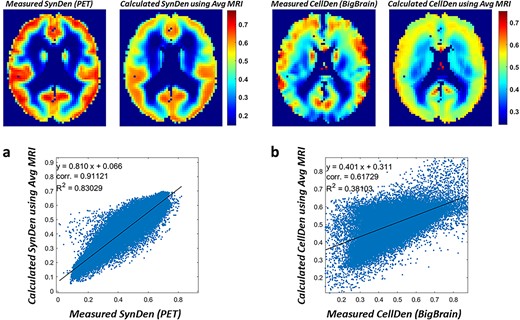
Neuropil predictions when trained on individual MRI data and high-smoothing. For the a) SynDen and b) CellDen predictions, the data from Supplementary Figure S1 were provided as inputs for the ANN model (Supplementary Figure S1). The network was trained to predict the in vivo PET SynDen reference standard (n = 30) for each of the 10 subjects with MRI data. The network was also trained to predict the ex vivo histology-based BigBrain/CellDen (n = 1) reference standard for each of the 10 subjects with MRI data. Data from 3 subjects were randomly set aside for validation purposes to prevent overfitting. The PET-measured SynDen dataset (top left, a) is compared with the ANN predictions (top right, a), and shows a high correlation (bottom, a). The ex vivo histological dataset (top left, b) is compared with the ANN predictions (top right, b), and shows a moderate correlation (bottom, b).
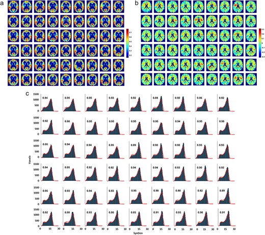
a) Predictions of normalized individual SynDen for each of the 54 ADNI test subjects using the individually trained high-smoothing ANN model. Cubic Gaussian-smoothing sigma |${\sigma}^3$| used for the network are 0, 1, 8, 64, and 512. Order of ADNI subjects same as in Supplementary Table S1. The individual predictions show the range and spatial patterns expected, showing that the ANN is not overfitting the data. However, the individual predictions were closer to the mean value throughout the brain, with standard deviations ranging from 0.13 to 0.15, compared to 0.16 in the reference standard dataset, which reflects the challenge of predicting the same SynDen reference standard regardless of ADNI subject with low mean squared error, while also providing evidence that our chosen network architecture is not overfitting the data, providing individualized predictions instead. Given our expectation that the ANN was predicting values closer to the mean due to an artificial inflation of the mean squared error as a result of the lack of individualized synaptic datasets for training, we normalized the data to correct for mean and standard deviation. Overall, spatial correlations of the subject predictions with our reference standard range from 0.83 to 0.91, averaging 0.89 across subjects. b) Absolute difference maps for the 54 subject SynDen predictions compared to the reference standard. Differences in SynDen predictions do not show a consistent pattern, which suggests that the prediction deviations are mainly individual variations. Of note however is that overestimations (in red) seem to be mainly limited to white matter regions, while underestimations (in blue) seem to be more localized to gray matter regions. While the figure shows that our ANN SynDen predictions are consistently lower in white matter and higher in gray matter as we expect from the reference standard, further efforts at fine tuning of the network may be possible to correct these under- and over-estimations in gray and white matter, respectively. It is also possible that with individualized datasets the network can be trained to predict individualized SynDen more effectively, thereby mitigating these observed systemic differences. Another possibility is that these systemic differences in gray and white matter are real individual variations, and arise because SynDen is already low in white matter and individual variations can for the most part only increase SynDen, with the reverse being true for gray matter. c) The associated SynDen histograms for the individual predictions with the continuous red lines showing the reference standard histogram, with individual subjects presented in the same order. The x axis is in the original (relative) scale of image intensities before normalization for ANN training. The fractional overlap of the prediction histogram for each subject with the reference standard is displayed on each histogram. The overlap between subject SynDen histogram predictions with the reference standard is high, ranging from 0.88 to 0.97, averaging 0.93 across subjects, demonstrating that our predictions achieve the range and spatial patterns expected.
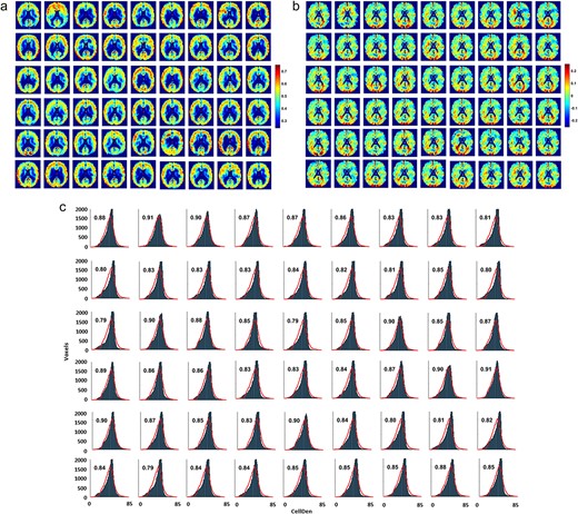
a) Predictions of normalized individual CellDen for each of the 54 ADNI test subjects using the individually trained high-smoothing ANN model. Cubic Gaussian-smoothing sigma |${\sigma}^3$| used for the network are 0, 1, 8, 64, and 512. Order of ADNI subjects same as in Supplementary Table S1. As with the SynDen predictions, the same ANN architecture predicts the range and spatial patterns expected for CellDen. Predictions were closer to the mean with lower standard deviation than in the reference standard, to a greater degree than present in the SynDen predictions, with standard deviations ranging from 0.063 to 0.093, compared to 0.16 in the reference standard dataset, reflecting the challenge of predicting the same CellDen reference standard regardless of ADNI subject and demonstrating low overfitting. Similar to the SynDen results, we normalized the data to correct for mean and standard deviation, presumably low as a result of our lack of individualized reference standards for each subject. This achieves predictions that are qualitatively very similar to our ex vivo histology-based reference standard. Overall, spatial correlations of the subject predictions with our reference standard range from 0.44 to 0.65, averaging 0.58 across subjects. b) Absolute differences in CellDen predictions for the 54 subjects compared to the reference standard. The patterns of over- and under-predictions with respect to the reference standard seem to show more similar patterns to each other than for the SynDen predictions. For example, patterns of over- and under-predictions in the visual cortex area (bottom of the slices shown near the visual cortex area) are highly conserved between subjects. On the one hand, this is evidence that our ANN is not overfitting the data due to spatial information inadvertently provided in the training datasets, in addition to MPRAGE, ADC, and FA information, since then the network could have learned away these systematic deviations correcting its prediction in the visual cortex area. One possible reason for these systematic deviations from the reference standard is that the CellDen reference standard, which was from a single subject, is not representative of the population at large (a problem which was not present with the SynDen reference standard, which was a group average). It could be that the network did indeed learn the appropriate relationships to predict CellDen from the limited data that it was provided, and systematically predicts “individual differences” from the reference standard for the 54 subjects, when in reality the individual differences is present in the single subject reference standard. c) The associated CellDen histograms for the individual predictions with the continuous red lines showing the reference standard histogram, with individual subjects presented in the same order. The x axis is in the original (relative) scale of image intensities before normalization for ANN training. The fractional overlap of the prediction histogram for each subject with the reference standard is displayed on each histogram. The overlap between subject CellDen histogram predictions with the reference standard range from 0.79 to 0.91, averaging 0.85 across subjects, demonstrating that, similar to our SynDen predictions, our CellDen predictions achieve the range and spatial patterns expected.
We used our trained ANNs to calculate the individual SynDen predictions for each of the 54 test subjects (Fig. 4a), where the normalized data from a representative slice are shown in Fig. 4a, with the respective SynDen difference maps from the reference standard in Fig. 4b and histograms in Fig. 4c. SynDen differences showed no clear pattern between test subject predictions, suggesting individual predictions. The individual SynDen histogram overlaps well to our reference standard SynDen histogram, ranging from 0.88 to 0.97 (i.e. averaging 0.93 across all 54 subjects; Fig. 4c). The lower spatial correlations of the reference standard SynDen and subject SynDen prediction images ranged from 0.83 to 0.91 (i.e. averaging 0.89 across all 54 subjects; Fig. 4a), demonstrating individualized variations of SynDen compared to the reference standard SynDen. However, the individual SynDen predictions were closer to the mean value throughout the brain with standard deviations ranging from 0.13 to 0.15, compared to 0.16 in the PET-measured SynDen reference standard dataset. This presumably reflects the challenge of predicting the same SynDen reference standard regardless of ADNI subject with low mean squared error, while also providing evidence that our chosen network architecture is not overfitting the data instead predicting individualized results. Due to data availability limitations, our networks were trained on individual MRI data as input with neuropil density from separate subjects as output; the calculated mean squared error were likely artificially inflated compared to a scenario where individualized neuropil densities are used for training. To emphasize the learned relationships over minimizing mean squared error, we normalized the individual predictions to match mean and standard deviations in measured neuropil data (Fig. 4a) to achieve SynDen predictions that are subjectively very similar to our PET-measured SynDen reference standard (Fig. 4c).
We repeated the same process described above (for SynDen) to also calculate the individualized CellDen predictions for each of the 54 test subjects using the ANN (Fig. 5a). Similar to findings for normalized individualized SynDen in Fig. 4a, the normalized individualized CellDen predictions showed comparable personalized heterogeneity representative of person-to-person variation. However, patterns in the variations from the reference standard (Fig. 5b) show some consistency between individuals such as in the visual cortex area. Given that the reference standard is from a single subject, this could be due to individual variations in the reference standard which deviate from the population at large. The individual CellDen histograms on the other hand overlap well with the reference standard CellDen histogram, with the overlap fraction ranging from 0.79 to 0.91 (i.e. averaging 0.85 across all 54 subjects; Fig. 5b). The lower spatial correlations of the reference standard CellDen and subject CellDen prediction images ranged from 0.44 to 0.65 (i.e. averaging 0.58 across all 54 subjects; Fig. 5c), demonstrating individualized variations of CellDen compared to the reference standard CellDen. Prediction standard deviations ranged from 0.063 to 0.093 compared to a standard deviation of 0.13 for the reference standard, necessitating normalization.
To see if we could circumvent the lack of individualized neuropil densities for each subject, in addition to our 2 final ANN models we also trained 4 additional networks (see Table 1 for the overall summary of all 6 ANN models) using group average MRI with both low-smoothing (|${\sigma}^3$| of 0, 0.5, 1, 2, and 4) and high-smoothing (|${\sigma}^3$| of 0, 1, 8, 64, and 512). While training on group average MRI on highly smoothed or mildly smoothed MRI data showed higher correlations between measured and calculated group average SynDen (Supplementary Fig. S2 with high-smoothing; Supplementary Fig. S3 with low-smoothing) and calculated group average CellDen (Supplementary Fig. S4 with high-smoothing; Supplementary Fig. S5 with low-smoothing), they were not very effective in predicting the individualized differences in neuropil density across the subjects. The networks trained on highly-smoothed group average MRIs performed quite poorly with individualized predictions due to overfitting and extrapolation errors when presented with the range of variability seen in individual MRI data. Networks trained on mildly smoothed group averages avoided the high overfitting and extrapolation errors present in the networks trained on highly-smoothed MRI, likely because the lack of highly-smoothed inputs forced the network to train on variations found within the group average, allowing it to extrapolate more effectively to individual variations. However, the individualized predictions had very low spatial autocorrelation (i.e. they were grainy and not as smooth) compared to the reference standards, which is why we rejected this approach. Avoiding this tradeoff in prediction efficacy necessitated us to maintain the training on highly-smoothed individual MRI data, and instead of addressing the overfitting issue by training on mildly smoothed data, to address it by training on individual data instead of group averages only, which is the approach used in our 2 final ANN models. While this individual subject training approach produced predictions that were qualitatively similar to our reference standards, it is subject to the limitation that we did not have corresponding individual CellDen and SynDen datasets for each of the ADNI subjects and had to assume the group average (for SynDen) or single subject (for CellDen) dataset for each ADNI subject. While our results identify that this kind of ANN architecture and individualized subject network training can potentially be used to predict CellDen and SynDen, future studies would need individualized datasets for more robust training of these networks.
By averaging all the individualized predictions of SynDen (Fig. 4a) and CellDen (Fig. 5a), we compared measured and calculated neuropil density in human brain (Fig. 6). The histograms of reference standard SynDen (Fig. 6a, top) and predicted SynDen (Fig. 6a, bottom) showed excellent match with histogram overlap of 0.93 and a high spatial image correlation of 0.91. The histogram of reference standard CellDen (Fig. 6a, top) and predicted CellDen (Fig. 6b, bottom) also demonstrated outstanding equivalence with a similarly high histogram overlap of 0.85 and a high spatial image correlation of 0.62. These values are in line with the average values found on the individual subject predictions as previously mentioned.
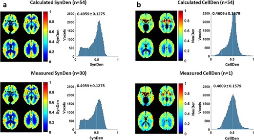
Comparison of measured and calculated neuropil density in human brain. a) Comparison of calculated SynDen (n = 54; all test subjects from ADNI) and measured SynDen (n = 30; all subjects from Finnema et al. 2016) in terms of images and histograms. Histogram of reference standard SynDen (bottom) and predicted SynDen (top) show excellent match with histogram overlap of 0.94. Average and standard deviation of SynDen shown on histogram. The reference standard was scaled so that mean SynDen is around 0.5 to facilitate ANN training, while the ANN output was normalized to match the reference standard mean and standard deviation. b) Comparison of calculated CellDen (n = 54; all test subjects from ADNI) and measured CellDen (n = 1; subject from Amunts et al. 2013) in terms of images and histograms. Histogram of reference standard CellDen (bottom) and predicted CellDen (top) show high match with histogram overlap of 0.84. Average and standard deviation of CellDen shown on histogram. The reference standard data was scaled so that average CellDen is around 0.5, with the ANN output normalized to match the reference standard mean and standard deviation.
Discussion
Study motivation
Neuropil consists of neuronal/glial cell bodies whose finest filaments (neuronal axons/dendrites and astrocytic filipodia) form synapses, and combines both CellDen (i.e. number of neuronal and glial cells) and SynDen (i.e. mass of microfilaments), as shown schematically in Fig. 1. Thus, neuropil represents the cellular unit (i.e. the hardware) within which the generated electrical signals are processed (i.e. the software). Neuronal and glial cells collaborate to produce the energy for unremitting operation of electrical signaling in the neuropil. Both neuropil density (i.e. the hardware) and electrical activity (i.e. the software) contribute to the brain’s metabolic heterogeneity.
Neuropil density is a fundamental component of metabolic function, and decreases in neuropil density are associated with disorders such as depression, Parkinson’s, Alzheimer’s, and aging (Flood and Coleman 1988; Scheff et al. 1990; Morrison and Hof 1997; Masliah et al. 2006; Martinez-Pinilla et al. 2016; Holmes et al. 2019; Matuskey et al. 2020). Neuropil density represents the microscopic infrastructure that regulates function which can be measured at the mesoscopic level (i.e. millimeter-sized voxels in the human brain). In spite of advances in metabolic and functional imaging (Hyder and Rothman 2017), the contribution of neuropil density to brain energetics has been difficult to account for. Conventional fMRI, a popular functional imaging modality, measures blood oxygenation changes in the brain which underlies blood flow response to changing oxidative demand or CMRO2 (Hyder and Rothman 2012). Calibrated fMRI can extract the CMRO2 quantitatively, albeit at mesoscopic resolution (Herman et al. 2013). PET metabolic imaging can also be used to measure CMRglc(ox) (Mortensen et al. 2018). Such metabolic measurements themselves, however, are only a rough proxy for neural firing rates (Yu et al. 2018). Relating bottom–up energy budgets accounting for neuropil density and top–down energetic measurements from PET and/or calibrated fMRI provides a connection between mesoscopic metabolism and microscopic anatomy to provide deeper understanding of brain function (Yu et al. 2023).
MRI data selection and machine learning
We used several selection criteria to narrow the MRI data available from ADNI (see Materials and methods). We limited subjects to those that were scanned using the ADNI 3 protocol, the latest scanning protocol in the ADNI project. Analysis was limited to those subjects that were scanned on Siemens 3T scanners, which are known to perform stably across sites, so as to maintain consistency between the datasets used. The ages of the subjects ultimately selected for this study ranged from the late 50s to early 80s, but otherwise healthy.
Various approaches were used to try to predict neuropil density from the MRI data, but the one we settled on and present in this paper uses an ANN that runs on a voxel-by-voxel basis, with nondirectional neighborhood information provided through additional isotropically-smoothed datasets as inputs to the ANN. Given that this ANN architecture was promising, we did not use a convolutional ANN, which would have access to richer neighborhood information in the MPRAGE, ADC, and FA datasets but with increased risk of overfitting, especially considering the nontraditional training regimen used due to dataset limitations, a risk which may not have been fully eliminated by validation. The number of nodes for the network at each layer was hand selected with the aim of choosing enough nodes to provide the algorithmic complexity to handle different dataset relationship cases while reducing the overfitting risk inherent in ANNs with large numbers of nodes. To improve the robustness of our ANN we used ensemble averaging as described in Materials and methods.
One of our training strategies averaged the 10 subject MPRAGE, ADC, and FA data to create group averages, and used the BigBrain cellular density or group average PET synaptic density as outputs. The reasoning behind using group averages was to overcome the limitation of having different subjects providing the input and output datasets for the ANN training, by using atlases for both input and output during training. While this training strategy was largely successful for group average prediction (Fig. S3 and S5), individual predictions performed poorly, likely as the full per subject variability within individual MPRAGE, ADC, and FA data were not considered during group average training and the ANN was unable to extrapolate to individual cases. Normalization of neuropil predictions from the ANN to match the standard deviation of our reference standards did not markedly improve the results. Training on less-smoothed data avoided the extrapolation errors (Fig. S4 and S6) but resulted in noisier predictions, likely as lower smoothing for the MRI inputs resulted in noisier input data for the ANNs to work with.
These results prompted us to use our preferred training strategy, which involved providing the individual subject MPRAGE, ADC, and FA datasets as inputs while predicting our reference standards as outputs regardless of subject during training (Fig. 4 and 5). When networks trained in this manner were provided individual MPRAGE, ADC, and FA data the individualized neuropil predictions were much more reasonable, albeit with smaller standard deviations that those seen in the reference standards, suggesting that the ANN was unable to find strong relationships between individual MPRAGE, ADC, and FA and reference standard neuropil density that minimized mean square error of the predictions. Since our goal was to predict individualized neuropil density based on these learned general relationships, we normalized the neuropil predictions to match the standard deviation of our reference standards. While we did not have the individual neuropil densities of the ADNI subjects for comparison, the resulting normalized predictions were comparabe to our reference standard datasets (Fig. 3 to 5A).
We used different levels of isotropic Gaussian smoothing to provide our ANN nondirectional neighborhood information. Providing low levels of Gaussian-smoothed datasets resulted in grainy neuropil predictions which deviate from what we observe in the reference standards, showing the importance of neighborhood information. Neighborhood information would also help to mitigate issues due to noisy datasets (by averaging out the noise) and any minor misregistration errors. Additionally, smoothed datasets can also provide a regional basis to calculate relative changes in MPRAGE, ADC, and FA by the ANN if so required for neuropil prediction.
Our ANNs were able to predict synaptic density more reliably than cellular density. This may reflect the simpler relationships for SynDen, which is distinct for gray and white matter. It may additionally reflect that fact that our reference standard SynDen was a group average and thus potentially more representative of the general population than our cellular density dataset which came from a single subject.
Limitations
Given dataset limitations of various kinds, this was a feasibility study to assess whether training with individual neuropil densities would be successful. Since the same reference standard neuropil density maps were assumed for all 10 subjects, proper validation was not feasible, and care was employed to avoid overfitting. Instead of using a convolutional ANN, we looked for the simplest network architecture with the fewest free parameters that could predict neuropil densities, resulting in the shallow fully-connected network with predefined Gaussian-smoothing kernels we present here. The specific image preprocessing Gaussian-smoothing kernels and machine learning ANN architecture presented here represent the culmination of various iterations of simple convolution filters, regressions, and artificial ANN machine learning approaches to find the simplest algorithm that can successfully predict probabilistic yet individualized neuropil densities.
Additionally, the predefined Gaussian smoothing/convolutions would typically reduce the intensity of the images near the brain edge due to voxels with zero intensity located outside the brain, thus potentially providing the network with spatial information (i.e. distance from the brain edge). This would potentially enable the network to “memorize” the target neuropil density based on this encoded spatial information, a particular problem since we only trained on 1 set of reference standard neuropil density maps. This concern was mitigated by normalizing the smoothed images with the equivalent smoothed binary mask images (see Materials and methods).
For future network training, having individual neuropil densities for network training would be optimal. This means having SynDen, CellDen, and MRI data from the same subjects. Although SynDen can be measured in vivo by PET, CellDen was measured ex vivo. There are some possibilities of advanced DWI methods, beyond the conventional diffusion tensor imaging (DTI) models, that could be used to measure CellDen in vivo. Such advanced DTI methods (Zhang et al. 2012) like neurite orientation dispersion and density imaging (NODDI) could play a significant role in future experimental plans. Similarly, a recently introduced in vivo MRI method called metabolic activity diffusion imaging (MADI) by Springer et al. (Springer et al. 2023b) suggests that a cellular density map across GM/WM can be obtained from DTI images based on Monte Carlo random walks in virtual stochastically sized/shaped cell ensembles. Early demonstration of the MADI method (Springer et al. 2023a) shows similar level of cellular density difference between GM/WM (Yu et al. 2018).
The input to our ANN model always consists of all structural imaging data, while the output comprises only 1 of the 2 single gold-standard maps. However, an ultimate goal could be an integrated neuropil map with a ratio of cells to synapses per voxel with joint training. Joint training is also possible where the same network and same initial layers of nodes are trained to predict CellDen and SynDen, but only the output layers are different to predict the different parameters. We have tried this approach and our initial attempts did not produce good predictions. CellDen and SynDen distributions seemed to be very different and thus seemed to require completely different, separately trained networks to predict as done here.
With our current training regimen, one limitation was the difference in ages of the different subjects. The MPRAGE, ADC, and FA from the ADNI project were from subjects in their late 50s to early 80s, but otherwise healthy. SynDen was a group average from subjects in their 20s, while CellDen was from a 65-year-old female. While the MRI and CellDen dataset were age-matched, the same was not true for the SynDen dataset. Age- and/or gender-dependent changes in neuropil density were thus not accounted for in the present study. Future studies, with careful planning of both anatomical and metabolic scans, would be warranted to avoid these limitations. Nonetheless, while outside the scope of this study, the currently trained networks can be run as is on subjects across different ages and genders (or even neurological conditions) to identify changes across these parameters. While the dataset used in this study includes only cognitively normal subjects, it does include age ranges from subjects in their 50s to subjects in their 80s. However, most subjects are in their 60s and 70s, presenting a very narrow age range, while subjects in their 50s and 80s are very few in number, raising concerns of statistical power with the current dataset.
Conclusion
With the approach used in this paper there is a need for validation on individually collected neuropil density datasets, as well as their individualized metabolic scans. This would ideally involve the collection of MPRAGE, ADC, and FA data as well as neuropil densities from the same subjects. One approach to do this in vivo could involve NODDI or MADI data for CellDen, as mentioned above, but also SynDen using PET in the same subject. Per subject, CMRglc(ox) can be either measured by a multi-modal PET method (Hyder et al. 2016), or alternatively CMRO2 can be measured via calibrated fMRI (Chen et al. 2022). Ideally, these individualized anatomic and metabolic datasets can then be used to run the brain energy budget model on a per subject basis (Yu et al. 2023) to provide understanding and quantification of microscopic effects underlying mesoscopic measures of brain function (Fig. 1).
Acknowledgements
Appreciation to Dr. Richard Carson of the Yale PET Center for access to the SynDen dataset. Thanks to Brian Chang for helpful reading of the manuscript. We are grateful to the reviewers for their constructive comments.
Author contributions
Adil Akif conceptualized research and wrote and vetted the software for analysis of the data, Fahmeed Hyder conceptualized research and vetted the software for analysis of the data, and Lawrence Staib conceptualized research and vetted the software for analysis of the data. All authors formally analyzed the data and wrote the original and revised manuscript.
Funding
Thanks to NIH funding to FH (R56 AG079086, R01 MH067528, R01 NS100106). Data collection and sharing for this project was funded by the Alzheimer’s Disease Neuroimaging Initiative (ADNI) (National Institutes of Health Grant U01 AG024904) and DOD ADNI (Department of Defense award number W81XWH-12-2-0012). ADNI is funded by the National Institute on Aging, the National Institute of Biomedical Imaging and Bioengineering, and through generous contributions from the following: AbbVie, Alzheimer’s Association; Alzheimer’s Drug Discovery Foundation; Araclon Biotech; BioClinica, Inc.; Biogen; Bristol-Myers Squibb Company; CereSpir, Inc.; Cogstate; Eisai Inc.; Elan Pharmaceuticals, Inc.; Eli Lilly and Company; EuroImmun; F. Hoffmann-La Roche Ltd and its affiliated company Genentech, Inc.; Fujirebio; GE Healthcare; IXICO Ltd; Janssen Alzheimer Immunotherapy Research & Development, LLC.; Johnson & Johnson Pharmaceutical Research & Development LLC.; Lumosity; Lundbeck; Merck & Co., Inc.; Meso Scale Diagnostics, LLC.; NeuroRx Research; Neurotrack Technologies; Novartis Pharmaceuticals Corporation; Pfizer Inc.; Piramal Imaging; Servier; Takeda Pharmaceutical Company; and Transition Therapeutics. The Canadian Institutes of Health Research is providing funds to support ADNI clinical sites in Canada. Private sector contributions are facilitated by the Foundation for the National Institutes of Health (www.fnih.org). The grantee organization is the Northern California Institute for Research and Education, and the study is coordinated by the Alzheimer’s Therapeutic Research Institute at the University of Southern California. ADNI data are disseminated by the Laboratory for Neuro Imaging at the University of Southern California.
Conflict of interest statement: FH is the founder of InnovaCyclics LLC. He has an equity interest in InnovaCyclics LLC, which is a biotechnology company creating next generation MRI contrast agents. All other authors declare no conflict of interest.
Data availability
Please direct all requests for data and software to FH.