


Abstract
It is important to explore causal relationships in functional magnetic resonance imaging study. However, the traditional effective connectivity analysis method is easy to produce false causality, and the detection accuracy needs to be improved. In this paper, we introduce a novel functional magnetic resonance imaging effective connectivity method based on the asymmetry detection of transfer entropy, which quantifies the disparity in predictive information between forward and backward time, subsequently normalizing this disparity to establish a more precise criterion for detecting causal relationships while concurrently reducing computational complexity. Then, we evaluate the effectiveness of this method on the simulated data with different level of nonlinearity, and the results demonstrated that the proposed method outperforms others methods on the detection of both linear and nonlinear causal relationships, including Granger Causality, Partial Granger Causality, Kernel Granger Causality, Copula Granger Causality, and traditional transfer entropy. Furthermore, we applied it to study the effective connectivity of brain functional activities in seafarers. The results showed that there are significantly different causal relationships between different brain regions in seafarers compared with non-seafarers, such as Temporal lobe related to sound and auditory information processing, Hippocampus related to spatial navigation, Precuneus related to emotion processing as well as Supp_Motor_Area associated with motor control and coordination, which reflects the occupational specificity of brain function of seafarers.
Introduction
Functional magnetic resonance imaging (fMRI) is a technology that reveals brain functional activity regions by measuring changes in blood oxygenation levels. It is a non-invasive technique compared to other methods for studying brain neural activity, which has advantages with no radiation, non-invasiveness, and high spatiotemporal resolution (Logothetis 2008), so that it has been widely applied in many fields of brain study. Among them, the brain functional connectivity (FC) based on fMRI is a crucial manner to explore the complex interactions and information transfer within the brain, which can be categorized into two types: FC and effective connectivity (EC; Chang and Glover 2010). FC is a undirected correlation analysis in temporal domain, which reveals the direct interaction between different brain regions(Woodworth et al. 2018). While EC is a directed correlation analysis that reveals the direction of information transmission and the causal relationship between different regions (Schlösser et al. 2008), which can help us to understand the functional organization of brain more comprehensively.
Among them, the information-theoretic method is considered an effective way of EC analysis, such as transfer entropy (TE) and mutual information (Wing et al. 2016), which has become an indispensable tool to reveal the complexity of the brain’s internal activities and connectivity in the field of fMRI. For example, Ursino et al. (2020) used transfer entropy as an indicator of brain connectivity and analyzed its advantages and limitations with the help of neuron model (Ursino et al. 2020). Wu et al. (2021) used transfer entropy to analyze resting-state fMRI data (Wu et al. 2021), and emphasized the connections and differences between the observed transfer entropy pattern and previous studies. Zeng et al. (2023) described the difficulties and challenges of using transfer entropy for time-series causal inference (Zeng et al. 2023), and compared it with Granger causality analysis methods, causal network structure learning algorithms, and other methods to analyze their advantages and disadvantages. Multiple studies have demonstrated that the transfer entropy method has several drawbacks. For instance, when estimating in uncoupled systems, it may overestimate or underestimate the actual situation (Smirnov 2013), resulting in false causality. Additionally, this method requires a substantial amount of computation (Krakovská et al. 2018). Therefore, further refinements and optimizations of the transfer entropy method are necessary to enhance its accuracy and computational efficiency.
Moreover, some studies use fMRI to investigate the relationship between brain neural activity and individual behavior, and to further explore the effects of occupational-related training or experience on individual behavior, which has become a crucial research direction in the field of cognitive neuroscience. For instance, Hervais-Adelman et al. (2015) conducted a study with individuals who had undergone simultaneous interpreting training (Hervais-Adelman et al. 2015) and found that these individuals exhibited plasticity in brain functionality, which correlated with the emergence of expert-level language control. Additionally, Shen et al. (2016) compared the brain FC patterns of professional taxi drivers and non-drivers (Shen et al. 2016), revealing significant differences in the alertness functional network, which could be utilized to distinguish between these two groups.
As a special occupational group, seafarers often experience prolonged separation from their families and work in confined spaces with high machine noise in challenging maritime environments (Shi and Zeng 2018). The unique and enduring nature of this profession results in significant differences on individual behavior and career experiences when compared to other occupational groups, leading to specific alterations in their brain neural activity. Shi et al. (2015) introduced a psychological health assessment method for seafarers based on fMRI through an in-depth examination of the default mode network (Shi et al. 2015), and then using support vector machines (SVM) as classifiers to identify sub-healthy seafarers. Due to the effects of the seafarers’ own physical and mental health changes on maritime operations safety, this aspect is also addressed in Shi et al’.s research (2019) (Shi et al. 2019). However, most of these studies belong to FC, without considering the direction between brain regions and the connection between seafarers’ brain regions under different brain templates.
Based on the above considerations, this paper introduce an asymmetric method based on transfer entropy for EC analysis, which enhances the accuracy of causal relationship detection by quantifying the information difference in forward and backward time predictions and adopts a normalized causal statistic for comparative purposes across different systems. Next, the proposed method is performed on the simulated data to demonstrate its effectiveness through comparisons with several traditional methods included Granger Causality (GC), Partial GC (PGC), Kernel GC (KGC), Copula GC, and traditional TE. Finally, it is applied for the fMRI data analysis of seafarers, and results unveil the impact of the special seafarers profession on brain functional activity.
Materials and methods
Transfer entropy
Conditional mutual information is the uncertainty reduction amount of one random variable, given another random variable. It measures the correlation between two random variables while considering the case of a given third random variables (Cover 1999). When the conditional mutual information is applied to a specific time series, the transfer entropy is obtained. Transfer entropy is non-parametric statistic measuring the amount of directed (time-asymmetric) transfer of information between two random processes. Transfer entropy from a process |$\mathrm{x}$| to another process |$\mathrm{y}$| is the amount of uncertainty reduced in future values of |$\mathrm{y}$| by knowing the past values of |$\mathrm{x}$|, given past values of |$\mathrm{y}$| (Schreiber 2000). More specifically, if |${\mathrm{x}}_t$| and |${y}_t$|for |$t\in \mathrm{N}$| denote two random processes, with the history of the influenced variable |${y}_{t-1:t-L}$| in the condition:
The inference of |$\mathrm{y}$| based on its past is defined as |$\mathrm{H}\left({y}_t|{y}_{t-1:t-L}\right)$| and the inference of |$\mathrm{y}$| based on the past of both |$\mathrm{x}$| and |$\mathrm{y}$| is defined as |$\mathrm{H}\left({y}_t|{y}_{t-1:t-L},{x}_{t-1:t-L}\right)$|. Figure 1 Shows the Venn diagram of |${TE}_{x\to y}$|, in which the blue portion represents the information from the past of |$\mathrm{x}$|, and the green represents the information from the past of |$\mathrm{y}$|. The orange represents the information from the values of |$\mathrm{y}$|, and the red part refers to the reduction in uncertainty of the value of |$\mathrm{y}$|, given the past of |$\mathrm{y}$| and obtains the past of |$\mathrm{x}$|, denoted as |${TE}_{x\to y}$|.
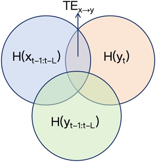
The Venn diagram of |${TE}_{x\to y}$|.
Asymmetric detection of TE
In this paper, the following statistic is used to make statistical inferences about causality from variables |$\mathrm{x}$| to |$\mathrm{y}$|, which is defined as information difference between forwards-in-time prediction and backwards-in-time prediction from |$\mathrm{x}$| to |$\mathrm{y}$|:
Where |$\eta >0$| presents the prediction lag, and |${\mathrm{TE}}_{\mathrm{x}\to \mathrm{y}}\left(\cdot \right)$| denotes the TE from |$\mathrm{x}$| to |$\mathrm{y}$|, which can be calculated as follows:
Therefore, the formula (2) can be converted into the following form:
For dynamical systems in general, the above definition in (2) can be understood as follows. Consider first the case of unidirectional coupling |$x\to y$|, then the influence that current values of |$x$| have on future values of |$y$| (forwards-in-time prediction) is expected to be stronger than the influence that current values of |$x$| have on past values of |$y$| (backwards-in-time prediction), i.e. |${TE}_{x\to y}\left(\eta \right)>{TE}_{x\to y}\left(-\eta \right)$| for every |$\eta >0$|. Hence, we expect |${\Delta }_{x\to y}\left(\eta \right)>0$| if |$x$| influences |$y$|. In the case of bidirectional influence |$x\leftrightarrow y$|, we expect that both |${\Delta }_{x\to y}\left(\eta \right),{\Delta }_{y\to x}\left(\eta \right)>0$|. Moreover, the relative magnitudes of |${\Delta }_{x\to y}\left(\eta \right)$| and |${\Delta }_{y\to x}\left(\eta \right)$| preserve the rank order of the underlying coupling strength. If |$x$| has no influence on |$y$|, then we expect no detectable influence neither directly from present |$x$| values to future |$y$| values, nor (because there is no interaction) from the present of |$x$| to its own future through its interaction with |$y$|. Therefore, |${\Delta }_{x\to y}\approx{\Delta }_{y\to x}\approx 0$|.
In order to calculate the transition probability in (5), consider a system that may be approximated by a stationary Markov process of order |$k$|, that is, the conditional probability to find |$y$| in state |${j}_{n+1}$| at time |$n+1$| is independent of the state in |${j}_{n-k}:p\left({j}_{n+1}|{j}_n,\cdots, {j}_{n-k+1}\right)=p\left({j}_{n+1}|{j}_n,\cdots, {j}_{n-k+1},{j}_{n-k}\right)$|. Henceforth, we will use the shorthand notation |${j}_n^{(k)}=\left({j}_n,\cdots, {j}_{n-k+1}\right)$| for words of length |$k$|, and similarly use |${i}_n^{(l)}=\left({i}_n,\cdots, {i}_{n-l+1}\right)$| for words of length |$l$| for |$x$|:
The most natural choices for |$l$| are |$l=k$| or |$l=1$|. Usually, the latter is preferable for computational reasons (Boba et al. 2015). In this case, the transfer entropy in formulas (3) and (4) can be estimated by the following equations, namely:
|${TE}_{x\to y}$| is now explicitly nonsymmetric since it measures the degree of dependence of |$y$| on |$x$| and not vice versa. By employing conventional binning methods, which involve partitioning the reconstructed state space (dividing the state space into discrete bins), and by statistically analyzing the frequency of trajectory visits to each bin (Lancaster et al. 2018), the invariant probability on that bin is estimated. Based on this invariant joint density, marginal density can be derived, and its transfer entropy is computed. When computing transfer entropy, the focus is on how much the uncertainty of the current state reduces given the past state conditions.
Given the significant variability in the estimated values of |$TE$| across different systems, a normalized causal statistic is introduced by integrating over the predicted spectra of the observed time series following the detection of transfer entropy asymmetry. This allows the comparison of relative magnitude of the predicted asymmetry between different systems:
where |${\mathrm{A}}_{x\to y}^{\mathrm{f}}$|can be regarded as a binary classifier for directional causal relationships. When |${\mathrm{A}}_{x\to y}^{\mathrm{f}}$|>|$\mathrm{f}$|, it indicates the detection of coupling from x to y (referred to as “forward”), and when |${\mathrm{A}}_{x\to y}^{\mathrm{f}}\le \mathrm{f}$|, it signifies the absence of interaction (referred to as “backward”).
In this method, the comparison of forward-time TE and backward-time TE is employed to prevent the generation of false causal. Backward-time TE is considered an intrinsic system property and is utilized to establish a testing baseline (Lancaster et al. 2018).
Results
Experimental data
Simulated dataset
To demonstrate the effectiveness and advantages of the transfer entropy based asymmetry detection method in nonlinear systems, the following experiments were conducted using simulated data generated from (Geweke 1984). Specially, three time series were generated based on the following equations, and each consisting of 4000 time points (Gourévitch et al. 2006). To minimize errors arising from random factors, each model is repeated 100 times to generate different simulation data:
There are three directed relationships in (10), including linear causal relationship (|${x}_2$|→|${x}_3$|) and nonlinear causal relationships (|${x}_1$|→|${x}_2$|, |${x}_1$|→|${x}_3$|), in which the nonlinearity degree of (|${x}_1$|→|${x}_2$|||${x}_3$|) is determined by parameter |$c$|, and |${\mathrm{\varepsilon}}_1$|, |${\mathrm{\varepsilon}}_2$|, |${\mathrm{\varepsilon}}_3$| denote the simulated Gaussian white noise, where their variances are equal to that of the original time series and the signal-to-noise ratio is 0 dB. In order to evaluate the detection performance of the proposed method for different nonlinear degrees of causal relationship x1 → x2|x3, three cases of c = 0.2, 0.5, and 0.9 are considered in the experiment.
Furthermore, in order to evaluate the detection ability of the proposed method for direct and indirect relationship, equation (10) is modified to equation (11) by removing the term of |$0.5{x}_1^2\left(n-1\right)$| in the third equation, and then three time series with 4000 time points are generated using (11):
where the meanings of all parameters are the same as those in (10). The causal relationships of |${x}_1$|→|${x}_2$| and |${x}_2$|→|${x}_3$| are exist, which indicating an indirect relationship of |${x}_1$|→|${x}_3$|. In addition, the parameter of |$c$| = 0.5 is setting in this case.
Apart from verifying the effectiveness and advantages of the transfer entropy-based asymmetric detection method in the above four simulated datasets within nonlinear systems, it also be compared to GC, PGC, KGC, CopulaGC, and |$TE$|.
Real-fMRI dataset
This study utilized resting-state fMRI data from 20 male professional seafarers recruited from a shipping company in Shanghai (aged between 42 and 57, mean age 49 years, all right-handed; Wang et al. 2017). These seafarers held various positions, including chief mate, helmsman, and seaman, and each had approximately 10–20 years of maritime experience. Meanwhile, 20 chinese male participants (aged 48–55, average age 51, all right-handed) recruited from land-based jobs in the university or secondary school campuses were used as the non-seafarer control group. All subjects in the non-seafarer group had neither navigation skills nor long-term experience at sea. The ages of the subjects in the two groups were matched and the education levels between them were equivalent. This study involving human participants received ethical approval from the Independent Ethics Committee of East China Normal University. All participants provided written informed consent and had no history of neurological or psychiatric disorders.
During the fMRI data acquisition process, all participants were instructed to maintain physical stillness, eyes closed, relaxed without thinking anything, awake and their ears were plugged with earplugs to reduce the effects of machine noise. The fMRI data acquisition was conducted at the Shanghai Key Laboratory of Magnetic Resonance of East China Normal College. The scanning protocol covers the whole brain with gradient echo planar imaging and provides 36 slices with a total of 160 volumes. The repetition time (TR) was set to 2.0 s, the scan resolution was 64 × 64, the plane resolution was 3.75 mm × 3.75 mm, and the slice thickness was 4 mm.
Data preprocessing
In this study, DPABI (http://rfmri.org/dpabi) was used to preprocess the fMRI data of seafarers and non-seafarers. Preprocessing includes the following steps: first, removing the first 10 time points in the fMRI data of each subject for magnetization equilibrium to compensate for transient scanner instability and participant’s adaptation to the circumstance. Then, slice timing, motion correction, spatial normalization, which standardizes the brain data of different subjects to the same size space, and spatial smoothing with the Gaussian kernel set to 4 mm, band-pass filtering(0.01–0.08 Hz), and detrending.
Next, the resting-state fMRI data of 20 seafarers and 20 age-matched healthy subjects are represented as seafarers’ group and non-seafarers’ group respectively. The following steps are performed for the two groups: firstly, each participant’s data was preprocessed, and then the signal values of all voxels within the corresponding brain regions were averaged based on the AAL template (Tzourio-Mazoyer et al. 2002) and the BrainnetToMe template (Fan et al. 2016), resulting in time series data for each Region of Interest (ROI). Subsequently, the asymmetry of transfer entropy is detected for each ROI time series of each subject, and each subject gets two causality matrices of 90 × 90 and 246 × 246, respectively. Finally, the statistical analysis of the results is conducted to identify ECs that are present in more than 80% of each group, and then analyzing the commonalities and individualities between the seafarer and non-seafarer groups, as well as the connections and distinctions under different brain templates in detailed.
Result analysis
Results of simulated data
The simulated data represents a multivariable nonlinear system, and its effectiveness is excellent in verifying the causal relationship of multiple conditions (Marinazzo et al. 2008; Farokhzadi et al. 2018). Additionally, the data encompasses both linear and nonlinear relationships, ensuring comprehensive consideration of different types of relationship. Figure 2 shows the results of state transition diagrams detected by ATE (Asymmetric Transfer Entropy), GC, PGC, KGC, CopulaGC, and TE on the four cases, respectively, in which the arrow pointing from |${x}_{\mathrm{i}}$| to |${x}_{\mathrm{j}}$| indicates that there is a causal relationship between them. It can be seen from the figure that the proposed ATE can detect all causal relationships in all four cases, and the detection effect is significantly better than other methods.
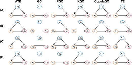
The state transition diagrams detected by ATE, GC, PGC, KGC, CopulaGC, and TE on the four cases, respectively. (A) The result of c = 0.5 in (10). (B) The result of c = 0.2 in (10). (C) The result of c = 0.9 in (10). (D) The result of c = 0.5 in (11).
For example, It can be seen from the results of case c = 0.5 shown in Fig. 2(A) that ATE, KGC, CopulaGC, and TE successfully identify causal relationships (|${x}_1$|→|${x}_2$|, |${x}_1$|→|${x}_3$|, |${x}_2$|→|${x}_3$|), while GC can only capture linear relationships (|${x}_2$|→|${x}_3$|), and PGC fails to accurately identify simple nonlinear relationships (|${x}_1$|→|${x}_3$|) and complex nonlinear connections (|${x}_1$|→|${x}_2$|). On the results of case c = 0.2 shown in Fig. 2(B), only ATE and CopulaGC can accurately identify causal relationships, and GC and PGC produce the same results as in (A). But KGC fails to accurately identify the complex nonlinear connection (|${x}_1$|→|${x}_2$|) when reducing the parameter c (i.e. reducing the nonlinearity of |${x}_1$|→|${x}_2$|||${x}_3$|), and TE also fails to capture the causal connection (|${x}_1$|→|${x}_2$|). On the results of case c = 0.9 as shown in Fig. 2(C), ATE and TE can accurately detect causality, and GC still cannot identify nonlinear connections, while PGC, KGC, and CopulaGC discover false causal connections (|${x}_3$|→|${x}_2$|). Lastly, on the results of case c = 0.5 using (11) shown in Fig. 2(D), ATE and TE successfully detect all causal connections, but other methods fail to accurately identify causal relationships.
Results of real-fMRI data
In this section, two templates of BrainnetToMe246 and AAL are involved (Tzourio-Mazoyer et al. 2002; Fan et al. 2016), in which the BrainnetToMe246 template divides the brain into seven major regions including Frontal lobe, Temporal lobe, Parietal lobe, Insular lobe, Limbic lobe, Occipital lobe, and Subcortical nuclei, while the AAL template divides the cerebral cortex of brain into 90 distinct regions. After using the proposed asymmetric detection of transfer entropy for the EC analysis of seafarer and non-seafarer groups, the brain regions corresponding to ECs that existed in at least 80% of subjects in each group were identified, and then ECs and related brain regions that existed in both BrainnetToMe and AAL templates were selected for further analysis.
Tables 1 and 2 show the brain regions selected from the AAL and BrainnetToMe templates and the associated information. It can be seen from these two tables that there is considerable correspondence between the brain regions selected from the two templates. Specifically, 32 brain regions selected from the BrainnetToMe template overlap with 36 brain regions selected from the AAL template, including Frontal_Sup_L, Precentral_L, Paracentral_Lobule_L, Temporal_Pole_Sup (L/R), Temporal_Mid_L, Temporal_Inf_R, and other areas. Next, the commonalities and individual characteristics between seafarers and non-seafarers are further investigated according to the frequency of occurrence of the selected ECs, which are shown in Tables 3–6.
Brain regions with high-connectivity effectiveness in AAL template.
| AAL Num | AAL regions | MNI coordinates | ||
|---|---|---|---|---|
| Frontal lobe | SFG | 3 | Frontal_Sup_L | (−19.5,34.8,42.2) |
| 20 | Supp_Motor_Area_R | (7.6,0.17,61.9) | ||
| PrG | 1 | Precentral_L | (−39.7,−5.7,50.9) | |
| 2 | Precentral_R | (40.4,−8.2,52.1) | ||
| PCL | 69 | Paraccentral_Lobule_L | (−8.6,−25.4,70.1) | |
| 70 | Paraccentral_Lobule_R | (6.48,−31.59,68.09) | ||
| Temporal lobe | STG | 83 | Temporal_Pole_Sup_L | (−40.9,15.1,−20.2) |
| 84 | Temporal_Pole_Sup_R | (47.3,14.8,−16.9) | ||
| 82 | Temporal_Sup_R | (57.2,−21.8,6.8) | ||
| MTG | 85 | Temporal_Mid_L | (−56.5,−33.8,−2.2) | |
| 86 | Temporal_Mid_R | (56.5,−37.2,−1.5) | ||
| ITG | 89 | Temporal_Inf_L | (−50.8,−28.1,−23.2) | |
| 90 | Temporal_Inf_R | (52.7,−31.1,−22.3) | ||
| PhG | 40 | ParaHippocampal_R | (24.4,−15.2,−20.5) | |
| Parietal lobe | SPL | 59 | Parietal_Sup_L | (−24.5,−59.6,58.96) |
| 60 | Parietal_Sup_R | (25.1,−59.2,62.1) | ||
| IPL | 61 | Parietal_Inf_L | (−43.8,−45.8,46.7) | |
| 62 | Parietal_Inf_R | (45.5,−46.3,49.5) | ||
| 64 | SupraMarginal_R | (56.6,−31.5,34.5) | ||
| Pcun | 67 | Precuneus_L | (−8.2,−56.1,48.0) | |
| 68 | Precuneus_R | (8.98,−56.1,43.8) | ||
| PoG | 57 | Postcentral_L | (−43.5,−22.6,48.9) | |
| Insular lobe | INS | 29 | Insula_L | (−36.1,6.7,3.4) |
| 30 | Insula_R | (38.0,6.3,2.1) | ||
| Occipital lobe | LOcC | 49 | Occipital_Sup_L | (−17.5,−84.3,28.2) |
| 43 | Calcarine_L | (−8.1,−78.7,6.4) | ||
| 44 | Calcarine_R | (15.0,−73.2,9.4) | ||
| 51 | Occipital_Mid_L | (−33.4,−80.7,16.1) | ||
| 52 | Occipital_Mid_R | (36.4,−79.7,19.4) | ||
| Subcortical nuclei | Hipp | 38 | Hippocampus_R | (28.2,−19.8,−10.3) |
| BG | 75 | Pallidum_L | (−18.8,−0.03,0.2) | |
| 76 | Pallidum_R | (20.2,0.18,0.23) | ||
| 73 | Putamen_L | (−24.9,3.9,2.4) | ||
| 71 | Caudate_L | (−12.5,11.0,9.2) | ||
| 72 | Caudate_R | (13.8,12.1,9.4) | ||
| Tha | 78 | Thalamus_R | (12.0,−17.6,8.1) |
Brain regions with high-connectivity effectiveness in BrainnetToMe template.
| BrainnetToMe Num | BrainnetToMe regions | MNI coordinates | ||
|---|---|---|---|---|
| Frontal lobe | SFG | 3 | SFG_L_7_2 | (−18,24,53) |
| 12 | SFG_R_7_6 | (6,38,35) | ||
| MFG | 20 | MFG_R_7_3 | (28,55,17) | |
| PrG | 57 | PrG_L_6_3 | (−26,−25,63) | |
| PCL | 65 | PCL_L_2_1 | (−8,−38,58) | |
| Temporal lobe | STG | 73 | STG_L_6_3 | (−50,−11,1) |
| 74 | STG_R_6_3 | (51,−4,−1) | ||
| MTG | 84 | MTG_R_4_2 | (51,6,−32) | |
| 85 | MTG_L_4_3 | (−59,−58,4) | ||
| 102 | ITG_R_7_7 | (54,−31,−26) | ||
| PhG | 114 | PhG_R_6_3 | (30,−30,−18) | |
| Parietal lobe | SPL | 125 | SPL_L_5_1 | (−16,−60,63) |
| 126 | SPL_R_5_1 | (19,−57,65) | ||
| IPL | 139 | IPL_L_6_3 | (−51,−33,42) | |
| 140 | IPL_R_6_3 | (47,−35,45) | ||
| Pcun | 147 | Pcun_L_4_1 | (−5,−63,51) | |
| 148 | Pcun_R_4_1 | (6,−65,51) | ||
| PoG | 159 | PoG_L_4_3 | (−46,−30,50) | |
| Insular lobe | INS | 163 | INS_L_6_1 | (−36,−20,10) |
| 164 | INS_R_6_1 | (37,−18,8) | ||
| Occipital lobe | LOcC | 205 | Locc_R_4_4 | (32,−85,−12) |
| Subcortical nuclei | Hipp | 218 | Hipp_R_2_2 | (29,−27,−10) |
| BG | 221 | BG_L_6_2 | (−22,−2,4) | |
| 222 | BG_R_6_2 | (22,−2,3) | ||
| 225 | BG_L_6_4 | (−23,7,−4) | ||
| 227 | BG_L_6_5 | (−14,2,16) | ||
| 228 | BG_R_6_5 | (12,5,14) | ||
| Tha | 237 | Tha_L_8_4 | (−7, −14,7) | |
| 241 | Tha_L_8_6 | (−15, −28,4) | ||
| 242 | Tha_R_8_6 | (13, −27,8) | ||
| 245 | Tha_L_8_8 | (−11, −14,2) | ||
| 246 | Tha_R_8_8 | (13, −16,7) |
Common effective connections in Seafarers and non-Seafarers groups under the AAL Template.
| AAL | Seafarers | Non-Seafarers | ||
|---|---|---|---|---|
| Number | ATE value | Number | ATE value | |
| Calcarine_R — > Calcarine_L | 18 | 0.901790652 | 17 | 1.252995329 |
| Putamen_L—> Caudate_L | 18 | 0.721675883 | 15 | 0.931529585 |
| Parietal_Inf_R—> Parietal_Sup_R | 17 | 0.733940484 | 14 | 0.939443104 |
| Parietal_Inf_L—> Parietal_Sup_L | 16 | 0.841810576 | 14 | 0.937616315 |
| Precentral_L—> Paraccentral_Lobule_L | 13 | 0.757688393 | 18 | 1.116238449 |
| Precentral_R—> Paraccentral_Lobule_R | 15 | 0.878871373 | 17 | 1.198241114 |
| Occipital_Sup_L — > Paraccentral_Lobule_R | 14 | 0.824402249 | 17 | 1.007194714 |
| Supp_Motor_Area_R — > Paraccentral_Lobule_R | 14 | 0.948737208 | 16 | 1.017588118 |
| Postcentral_L — > Paraccentral_Lobule_L | 14 | 0.939724392 | 16 | 1.220990116 |
Table 3 shows the information of common ECs in seafarers and non-seafarers of the AAL template, including the number of subjects in each group as well as their association strength. For example, the EC from Calcarine_R to Calcarine_L is typically involved in the processing, interpretation, and integration of visual information (Klein et al. 2000), which is considered a crucial area for visual information processing, contributing to the formation of human perception of the visual world. The EC from Putamen_L to Caudate_L, is helpful to regulate and coordinate body movements in both daily life and professional needs, which may be because thet both belong to Subcortical nuclei. The ECs from Parietal_Inf_L/R to Parietal_Sup_L/R is aiding in the collaboration between integrating perceptual information and higher-level cognitive processing. The ECs from Postcentral_L to Paracentral_Lobule_L provides sensory information (Iwamura et al. 1994), which may be utilized by the Paracentral lobule to adjust bodily movements in response to sensory stimuli. The others ECs are related to Paracentral lobule that is associated with sensory and motor control and is responsible for processing and coordinating movements, sensations, and coordination of the lower limbs and pelvis.
Table 4 shows the individual-specific ECs in AAL template, which are more present (>80%) in seafarers while less present in non-seafarers, such the ECs from Temporal_Mid_L/R to Precuneus_L/R and the EC from Temporal_Sup_R to Paracentral_Lobule_R. The middle and superior temporal gyrus are involved in auditory and language processing (Patterson et al. 2007), while the precuneus is associated with higher cognitive functions and self-awareness (Cavanna 2007). The paracentral lobule is responsible for sensory information transmission and motor control (Spasojević et al. 2013). Therefore, these ECs may help seafarers better adapt to complex auditory and language contexts, such as communication with crew members and control towers, receiving navigation instructions, completing daily tasks, and maintaining high levels of alertness. Furthermore, the insula plays a critical role in emotional processing and self-awareness (Craig 2009), while the superior temporal pole is involved in emotions and social cognition (Olson et al. 2002). Therefore, the ECs from Insula_L/R to Temporal_Pole_Sup_L/R may assist seafarers in better managing emotional challenges with colleagues and in their personal lives, as well as adapting to feelings of isolation and stress in both work and life.
Individual-specific effective connections in Seafarers group under the AAL Template.
| AAL | Seafarer group | Non-Seafarer group | ||
|---|---|---|---|---|
| Number | ATE value | Number | ATE value | |
| Pallidum_R — > Thalamus_R | 18 | 0.745165716 | 9 | 1.145348809 |
| Temporal_Mid_R — > Precuneus_R | 17 | 0.779448603 | 7 | 0.955787095 |
| Temporal_Sup_R — > Paraccentral_Lobule_R | 17 | 0.831984672 | 10 | 1.087264417 |
| SupraMarginal_R — > Paraccentral_Lobule_R | 17 | 0.728067434 | 8 | 0.859311048 |
| Pallidum_L — > Caudate_L | 17 | 0.725589225 | 9 | 0.915461898 |
| Pallidum_R — > Caudate_R | 16 | 0.742590643 | 8 | 0.938154062 |
| Insula_L — > Temporal_Pole_Sup_L | 16 | 0.757173888 | 11 | 1.075884653 |
| Insula_R — > Temporal_Pole_Sup_R | 16 | 0.693295817 | 8 | 0.912621807 |
| Temporal_Mid_L — > Hippocampus_R | 16 | 0.745493014 | 9 | 1.248936738 |
| Temporal_Mid_L — > Precuneus_L | 16 | 0.862281237 | 8 | 1.061873243 |
| Frontal_Sup_L — > Precuneus_R | 16 | 0.808383299 | 8 | 0.853944497 |
| Insula_R — > Supp_Motor_Area_R | 16 | 0.693035364 | 7 | 0.840687765 |
| ParaHippocampal_R — > Hippocampus_R | 16 | 0.831784276 | 10 | 1.021270863 |
| Pallidum_L — > Thalamus_R | 16 | 0.838144679 | 8 | 1.041982898 |
| Temporal_Inf_L — > Precuneus_L | 16 | 0.693056446 | 7 | 0.824541146 |
| Temporal_Inf_R — > Precuneus_R | 16 | 0.769674187 | 10 | 0.998780786 |
Table 5 shows detailed information of common ECs in seafarers and non-seafarers of the BrainnetToMe template, including the number of subjects in each group as well as their association strength. For example, the EC from BG_R_6_4 (i.e. ventromedial putamen) to BG_L_6_5 (i.e. dorsal caudate) is equivalent to the EC from Putamen_L to Caudate_L in the AAL template, as well as the ECs from IPL_L/R_6_3 (rostrodorsal area 40) to SPL_L/R_5_1 (rostral area 7) correspond to the ECs from Parietal_Inf_L/R to Parietal_Sup_L/R in the AAL template. Of course, there are also some ECs that are unique exist in the BrainnetToMe template in addition to these similar ECs, and they cannot be found in the AAL template. These unique ECs may reflect that the partitioning way of BrainnetToMe template is more sensitive the detection of ECs, leading to the discovery of some unique interactions between brain regions, such as the EC from the left lateral pre-frontal thalamus to the left rostral temporal thalamus.
Common effective connections in Seafarers and non-Seafarers groups under the BrainnetToMe Template.
| BrainnetToMe | seafarer group | Non-seafarer group | ||
|---|---|---|---|---|
| Number | ATE value | Number | ATE value | |
| BG_L_6_4 — > BG_L_6_5 | 17 | 0.898987008 | 15 | 0.864472793 |
| IPL_R_6_3 — > SPL_R_5_1 | 17 | 0.940898367 | 16 | 0.874596593 |
| IPL_L_6_3 — > SPL_L_5_1 | 17 | 0.934843825 | 16 | 1.201760871 |
| PoG_L_4_3 — > PCL_L_2_1 | 16 | 0.835368136 | 16 | 1.309547826 |
| Tha_L_8_8 — > Tha_L_8_4 | 18 | 0.900325029 | 17 | 1.000434326 |
Table 6 shows the individual-specific ECs in the BrainnetToMe template, which simlar to the results of AAL template in Table 4. For example, The ECs from INS_6_1_L/R (hypergranular insula) to STG_6_3_L/R (TE1.0 and TE1.2) correspond to the ECs from Insula_L/R to Temporal_Pole_Sup_L/R in the AAL template. The EC from MTG_L_4_3 (dorsolateral area 37) to Pcun_L_4_1 (medial area 7) corresponds to the ECs from Temporal_Mid_L/R to Precuneus_L/R in the AAL template. In addition, there are also some unique ECs in the BrainnetToMe template, such as EC from SFG_R_7_6 (medial area 9) to MFG_R_7_3 (area 46).
Individual-specific effective connections in Seafarers group under the BrainnetToMe Template.
| BrainnetToMe | Seafarer group | Non-Seafarer group | ||
|---|---|---|---|---|
| Number | ATE value | Number | ATE value | |
| BG_L_6_2 — > BG_L_6_5 | 18 | 0.953182204 | 10 | 1.005757996 |
| BG_R_6_2 — > BG_R_6_5 | 17 | 0.788397536 | 9 | 1.048823727 |
| INS_L_6_1 — > STG_L_6_3 | 17 | 0.807563605 | 10 | 0.981555708 |
| INS_R_6_1 — > STG_R_6_3 | 16 | 0.820063075 | 7 | 0.849829473 |
| MTG_L_4_3 — > Pcun_L_4_1 | 16 | 0.794871529 | 6 | 1.250339722 |
| SFG_L_7_2 — > Pcun_R_4_1 | 16 | 0.844554484 | 8 | 0.784484842 |
| PhG_R_6_3 — > Hipp_R_2_2 | 17 | 0.979981056 | 11 | 0.995165654 |
| ITG_R_7_7 — > Pcun_R_4_1 | 16 | 0.830147682 | 6 | 1.254868181 |
| Tha_L_8_8 — > Tha_L_8_6 | 17 | 0.885151703 | 10 | 1.116799475 |
| Tha_R_8_8 — > Tha_R_8_6 | 16 | 1.006788799 | 9 | 1.047739789 |
| PrG_L_6_3 — > Locc_R_4_4 | 17 | 0.840084161 | 11 | 1.279510465 |
| PhG_R_6_3 — > MTG_R_4_2 | 16 | 0.890293863 | 5 | 0.744651867 |
| SFG_R_7_6 — > MFG_R_7_3 | 16 | 0.839938901 | 9 | 1.041146826 |
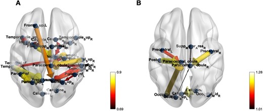
In the lower-right corner of Figs. 3–Fig. 5, a graduated color scale is presented, transitioning from lighter to darker hues. Lighter colors signify higher connectivity strength, while darker colors denote weaker connections. Additionally, the thickness of the connections also reflects the magnitude or strength of the values, with thicker lines denoting greater strengths, and thinner lines indicating weaker associations.
The effective connectivity networks for Seafarers and non-Seafarers groups on the AAL Template.
According to the screened ECs in the AAL and BrainnetToMe templates, the brain EC networks of seafarers and non-seafarers are constructed respectively, as shown in Figs. 3 and 4. Regardless of the brain template used, it can be seen from the figures that the ECs number of seafarers is obviously more than that of non-seafarers. Moreover, it was observed that the connectivity strength in non-seafarers brain regions was higher than those in seafarers.
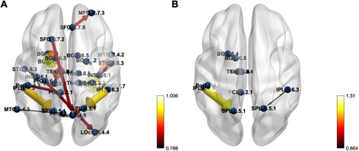
The effective connectivity networks for Seafarers and non-Seafarers group on the BrainnetToMe Template.
Finally, the brain ECs networks of seafarers corresponding to the AAL and BrainnetToMe templates are drawn respectively in Fig. 5. It can be seen clearly from the figure that there is a certain degree of consistency in the ECs among seafarers between the different brain templates, such as the Insula, Temporal_Sup, Parietal_Sup, Parietal_Inf, and others. Meanwhile, there are some differences due to the different partitioning way between the AAL and BrainnetToMe templates.
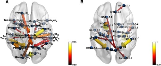
The effective connectivity networks for Seafarers group on both AAL and BrainnetToMe Templates.
Discussion
In response to the problems of traditional EC analysis methods, which are prone to false causal relationships and the need to improve detection accuracy, this paper introduces a method based on asymmetric detection of transfer entropy. This method quantifies the difference in predictive information between forward and backward time, and then normalizes this difference. Subsequently, it is demonstrated on simulated data that this method can more accurately detect causal relationships when compared to methods like GC, PGC, and so on. By applying this method to fMRI data from seafarers and non-seafarers, it was found that there was correspondence under different templates. After filtering effective connections and comparing the connectivity between seafarers and non-seafarers, significant differences were observed in specific brain regions. These differences were particularly pronounced in areas related to sound processing, spatial navigation, and emotional processing.
Based on the selected brain regions, it was observed that there is extensive correspondence between the BrainnetToMe and AAL templates. The brain regions selected under the AAL template, including the Frontal_Sup, Precentral, Paraccentral_Lobule, Temporal_Pole_Sup, Temporal_Mid, ParaHippocampal, Parietal_Sup, Precuneus, Postcentral, Insula, Hippocampus and more. All of them have corresponding regions in the BrainnetToMe template, which implies that they can be compared and associated across different brain templates, thus aiding in a more comprehensive understanding of the brain connectivity patterns and associated neural activity differences between seafarers and non-seafarers.
For example, it can be seen from Tables 3 and 5 that there are common connections within the brain regions such as the basal ganglia, thalamus, and cortex around the parietal fissure, indicating that there are common neural pathways between seafarers and non-seafarers in certain brain regions. These regions are core parts of the brain responsible for performing basic sensory and motor control functions, which are crucial for maintaining survival and adapting to different environmental conditions. In the brain regions related to sound, language, and auditory processing such as Temporal_Sup, Temporal_Mid, and Temporal_Inf (Rauschecker and Scott 2009; Wang et al. 2018), seafarers exhibit more pronounced brain region connections, and this may be due to the reason that they need to process various sound information, including communication, navigation, and environmental noise, due to their long-term work in noisy environments. This work environment leads to more sensitivity in these brain regions to help them cope with complex sound environments and language communication tasks more effectively.
When it comes to brain regions such as the Hippocampus, ParaHippocampal, and Thalamus (Okeefe and Nadel 1979; Epstein 2008; Saalmann and Kastner 2011), these regions play a key role in spatial navigation and place memory, mainly including the perception of the surrounding environment, the storage of location and path information, and the integration of different sensory inputs, which is helpful for effective navigation (Vantomme et al. 2020). For seafarers, performing complex navigation tasks in a complex maritime environment requires strong spatial perception and place memory skills. Therefore, compared to non-seafarers, there may be stronger effective connections in these brain regions. The Precuneus, SupraMarginal, and Insula are vital brain regions in emotion processing. Precuneus is involved in emotion regulation and conflict resolution (Cavanna 2007; Guendelman et al. 2022), SupraMarginal is implicated in emotion regulation and cognitive control (Devinsky et al. 1995; Wu et al. 2020), and Insula is associated with emotional experiences and self-awareness (Craig 2009). These brain regions play critical roles in monitoring psychological states and maintaining emotional health. Considering the unique profession of seafarers, who endure long separations from their families, live in relatively isolated environments, and cope with high levels of stress and emergency situations, these factors may lead seafarers to have more ECs among these brain regions. This enhanced connectivity may help them address the emotional and psychological challenges associated with their occupation.
The Supplementary Motor Area (Supp_Motor_Area) typically involves motor control and coordination (Nachev et al. 2008). For seafarers, dealing with navigation tasks and adapting to the maritime environment requires precise motor control and coordination. Therefore, this may result in seafarers having an increased number of effective connections in Supp_Motor_Area to better meet their occupational demands. By filtering with the same conditions, as shown in Fig. 3, the number of brain region connections for seafarers under the AAL template is 20, while that for non-seafarers is 8. Under the BrainnetToMe template, the number of brain region connections for seafarers is 18, while that for non-seafarers is 7. This difference may reflect the unique and consistent nature of the seafarer’s profession. Seafarers typically work in similar tasks and environments, which may lead to more uniform and enriched brain region connections, resulting in more effective connections. In contrast, non-seafarers engage in a wide variety of occupations, with more diverse brain connection patterns, resulting in relatively fewer connections. This finding highlights the potential impact of occupation on individual brain connectivity.
Acknowledgments
The content is solely the responsibility of the authors and there is no conflict of interest between the authors.
Author contributions
Yuhu Shi: Conceptualization, Methodology, Supervision, Writing—review & editing.Yidan Li: Formal Analysis, Visualization, Writing—original draft.
Funding
There is no funding support.
Conflict of interest statement: None declared.