


Abstract
Neuroimaging evidence implicates structural network-level abnormalities in bipolar disorder (BD); however, there remain conflicting results in the current literature hampered by sample size limitations and clinical heterogeneity. Here, we set out to perform a multisite graph theory analysis to assess the extent of neuroanatomical dysconnectivity in a large representative study of individuals with BD.
This cross-sectional multicenter international study assessed structural and diffusion-weighted magnetic resonance imaging data obtained from 109 subjects with BD type 1 and 103 psychiatrically healthy volunteers.
Whole-brain metrics, permutation-based statistics, and connectivity of highly connected nodes were used to compare network-level connectivity patterns in individuals with BD compared with controls.
The BD group displayed longer characteristic path length, a weakly connected left frontotemporal network, and increased rich-club dysconnectivity compared with healthy controls.
Our multisite findings implicate emotion and reward networks dysconnectivity in bipolar illness and may guide larger scale global efforts in understanding how human brain architecture impacts mood regulation in BD.
Introduction
Network science and graph theory have been increasingly employed to assess large-scale neuroanatomical dysconnectivity in debilitating brain disorders (Jiang 2013; Crossley et al. 2014) and can extend focal neuroanatomical neuroimaging studies to explore circuit-level white and gray matter organization. Although multiple indicators across a range of neuroimaging modalities report focal white matter pathophysiology in bipolar disorder (BD), research using graph theory techniques allowing networks to be assessed at a large scale of connectivity remains limited with inconsistent findings (Leow et al. 2013; Gadelkarim et al. 2014; Forde et al. 2015; Wang et al. 2018; Nabulsi et al. 2019).
Network analysis uses structural magnetic resonance imaging (MRI) and diffusion-weighted Imaging (DWI) to map the series of neuroanatomical elements (nodes) and their white matter connections (edges). Nodes are typically defined by cortical and subcortical gray matter regions, and the axonal bundles linking these nodes are derived via brain tractography. Graph theory properties of the brain are then employed to interpret features of integration and segregation within the series of interconnections or “connectome.” Measures of integration, including path length and efficiency, describe the shortest paths connecting nodes and can be interpreted at the nodal and whole-brain level (Bullmore and Sporns 2009). Subnetworks are interlinked regions with greater or lower connectivity within the network compared with regions outside the subnetwork giving rise to coordinated functions. The rich-club is an integrative connected subunit that is critical for coherent integration spanning multiple cortices (McAuley et al. 2007).
BD has been increasingly considered a “dysconnection syndrome” because of the complex interplay between gray and white matter components, predominantly involving emotion-regulatory and reward-related circuitries. The dysconnectivity hypothesis suggests that psychotic illnesses arise not from regionally specific focal pathophysiology, but rather from impaired neuroanatomical integration across networks of brain regions. To date, graph analyses investigations in BD report that abnormal global integration and dysconnected frontolimbic and interhemispheric connectivity may be trait features of BD (Leow et al. 2013; Collin et al. 2016; Roberts et al. 2018; Wang et al. 2018; Nabulsi et al. 2019). Disrupted global integration is consistent with the widespread reductions in white matter organization reported in BD (Vederine et al. 2011; Nortje et al. 2013; O’Donoghue et al. 2017a). Reduced frontolimbic and more posterior regional integration have been identified as features of BD in relatively small but clinically homogenous samples (Leow et al. 2013; Gadelkarim et al. 2014; Forde et al. 2015; Wang et al. 2018; Nabulsi et al. 2019). However, conflicting results in BD are not uncommon. For example, 4 studies reported preserved rich-club connectivity in BD (Collin et al. 2016; Roberts et al. 2018; Wang et al. 2018; Cea-Cañas et al. 2019), whereas both weak connectivity deficits (O’Donoghue et al. 2017b) and increased rich-club connectivity (Nabulsi et al. 2019) have been recently observed. Moreover, a trend of functional network-level changes of BD appears to involve specific functional subsystems that predominantly encompass default-mode network, limbic and reward centers, as opposed to being widespread (Wang et al. 2015, 2016; He et al. 2016; Manelis et al. 2016; Spielberg et al. 2016; Doucet et al. 2017; Wang et al. 2017b; Zhao et al. 2017; Roberts et al. 2017; Wang et al. 2017a; Zhang et al. 2019; Dvorak et al. 2019; Anand et al. 2020; Yang et al. 2020).
Multicenter studies may overcome the clinical heterogeneity of smaller samples to produce findings that are more generalizable to the true patient population and disambiguate conflicting findings from single-center studies by increasing statistical power (Ching et al. 2020). In an effort to reduce the biases associated with single center recruitment, the present study combined MRI data from 3 international centers, collected using identical acquisition protocols and scanners, to examine features of anatomical network connectivity in BD using data-driven graph theory techniques. Using a standardized neuroanatomical template, increased power, and clinically homogenous sample, we aimed to explore the topology of previously implicated neuroanatomical dysconnectivity in BD while comparing connectivity across both cortical and subcortical regions and connections relative to controls. This study builds from previous studies of structural and functional brain connectivity and brain network organization in BD and aims to further clarify unresolved questions related to the neurobiology of BD. We carried an exploratory investigation of the structural whole-brain and regional patterns of dysconnectivity in BD relative to controls, including rich-club connectivity and rich-club membership. Building from previous structural studies, we anticipated that individuals with BD, relative to psychiatrically healthy controls, will exhibit abnormalities in the brain’s structural organization at the whole-brain level in terms of segregation and integration; both negatively affected in patients. We hypothesized that multiple subnetworks would be affected in BD, based on previously identified white matter abnormalities and connectome dysconnectivity in small monocentric studies in BD. Specifically, we anticipate aberrant patterns of subnetwork connectivity in BD involving specific localized subsystems that implicate nodes belonging to emotion-regulatory circuits systems—both negatively affected in patients relative to controls. Localized dysconnectivity, along with reductions in whole-brain connectivity, would support the hypothesis that neuroanatomical deficits of BD may be confined to specific anatomical subnetworks.
Materials and Methods
This collaborative study incorporated data collected at the following 3 centers: Western Psychiatric Institute and Clinic in Pittsburgh, Pennsylvania, United States of America; Neurospin Lab and Assistance Publique-Hôpitaux de Paris, France; and Central Institute for Mental Health in Mannheim, Germany. This coordinated research effort implemented identical scanner and image acquisition protocols, which together with recruitment and clinical assessment have been described in detail previously (Sarrazin et al. 2014). Briefly, participants were between 18 and 65 years of age and fulfilled criteria for BD type I (Bell 1994) during clinical interview with a psychiatrist by DSM-IV-R criteria. Healthy participants were recruited from media announcements and registry offices; their criteria included having no personal or family history of Axis-I mood disorder, schizophrenia, or schizoaffective disorder. Exclusion criteria for all participants included a history of neurological disease or traumatic brain injury with loss of consciousness, as well as any MRI contraindications.
Image Acquisition
DWI and structural T1-weighted scans were obtained for all participants using the same model 3 T Magnetom Triotim syngo MR B17 with 12-channel head coil from Siemens Medical Solutions. Structural MRI acquisition includes a high-resolution T1-weighted acquisition (echo time, 2.98 ms; repetition time, 2300 ms; 160 sections; voxel size, 1.0 × 1.0 × 1.0 mm). A DW sequence was acquired along 41 gradient directions (voxel size, 2.0 × 2.0 × 2.0 mm; b = 1000 s/mm2 plus 1 b = 0 image; echo time, 87 or 84 ms; repetition time, 14 000 ms; 60 or 64 axial sections).
Preprocessing
Preprocessing steps of diffusion data consisted of subject motion and echo-planar imaging correction (Leemans et al. 2009; Jones and Cercignani 2010). “ExploreDTI” software was used to perform subject and geometric distortion correction and quality assessment of diffusion MRI data across all centers (Leemans et al. 2009). Rigid-motion and eddy current induced-distortions were corrected with a 6-parameter remapping of DW images to structural scans. All images were visually inspected for potential artifacts. Visual inspection was carried out across all raw data, structural, and diffusion MRI, to check for poor acquisition, movement, susceptibility, and noise artifacts. The inspection of DW images was also carried out postprocessing to identify the following artifacts: geometric distortions, hypointensities, and signal dropout, across all 3 orthogonal views.
Tractography
White matter trajectories were reconstructed using nontensor deterministic streamline tractography method using ExploreDTI v.4.8.3 (Leemans et al. 2009). Extending DTI tractography reconstruction of the principle fiber orientation defined by the largest eigenvalue, constrained spherical deconvolution (CSD) modeled the multiple diffusion directions within each voxel as an ellipsoid (Tournier et al. 2007, 2011; Jeurissen et al. 2011). The CSD algorithm was implemented to account for crossing fibers present within voxels (Tournier et al. 2007; Jeurissen et al. 2011). Streamlines were terminated when the tractography angle reached > 30° as CSD can reliably resolve multiple diffusion orientations at small crossing angles (Tournier et al. 2008). In addition, recursive calibration of the response function accounted for partial volume effects present within voxels of multiple fiber orientation directions (Tax et al. 2014).
Edges and Nodes
Fractional anisotropy (FA) presents a voxel-wise index of microstructural organization in white matter that is averaged across the streamlines connecting 2 nodes. Streamline count has been the most commonly used edge weight in studies employing graph analysis (Fornito et al. 2013) and was used here in addition to FA. It is calculated through voxel-by-voxel changes in the diffusion orientation representing a fiber tract. White matter trajectories were reconstructed using the deterministic streamline tractography method using ExploreDTI v.4.8.3 (Leemans et al. 2009). A CSD algorithm was implemented to account for crossing fibers present within voxels (lmax = 6) (Tournier et al. 2007; Jeurissen et al. 2011). Following tractography reconstruction, structural connectivity matrices were generated using “ExploreDTI,” connecting the set of reconstructed streamlines with a structural parcellation atlas consisting of automated anatomical labeling atlas (AAL-90) coordinates, labels, and volumes (Tzourio-Mazoyer et al. 2002). Undirected 90 × 90 connectivity matrices were produced for each participant, and weighted by the average FA or the number of streamlines (NOS) between 2 nodes in the network (Fig. 1).
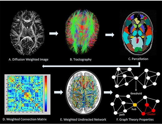
Network analysis methodological protocol. (A) Represents a diffusion MR image. (B) Tractography is carried out through ExploreDTI to delineate WM tracts; Genu of corpus callosum is shown. (C) Cortical and subcortical structure parcellation by AAL. (D) Weighted connectivity matrix. (E). Weighted undirected network. (F) Metrics used in BCT to characterize brain topology shows a network above and after thresholding only identifies stronger connections. (F) Describes a path indicated by the dashed line, a hub that highlights many interconnecting links is identified in yellow, and a cluster of nearest neighboring nodes is highlighted in red.
Global Metrics
Global parameters summarizing whole-brain connectivity properties of BD networks were derived from weighted structural matrices and included degree, characteristic path length, local and global efficiency, and clustering coefficient; calculated as the mean of the respective 90 regional estimates (Brain Connectivity Toolbox v1.52) (Rubinov and Sporns 2010). These measures can be divided into measures of integration, segregation, and influence (Sporns 2011). Characteristic path length and efficiency are measures of integration, reflecting the efficiency of communication through the network; with shorter paths and higher efficiency easing the distribution of information throughout the network. Clustering coefficient is a measure of segregation, providing information about the extent to which neighboring nodes share connections and create communities; whereby the more strongly interconnected nodes are, the more segregated and less sparse the network. Nodal degree is a measure of influence, whereby nodes with high degree are topologically central within a network. Statistical analyses of global metrics used linear mixed-effects models to account for any variance contributed by scanners employed at each of the 3 research centers and included research center as a random-effects factor. Age and sex were included as confounding variables.
Network-Based Statistics
The network-based statistics (NBS) toolbox was employed to detect a statistical group effect at the subnetwork level (Zalesky, Fornito, and Bullmore 2010). The NBS addresses the problem of multiple comparisons typically shown when comparing data across the series of interconnections between nodes. An F-test with a primary threshold of T > 2 was used to model differences between groups with additional covariates to account for research center, age, and sex and additionally tested for T > 1, T > 2.5, and T > 3. The permutation test ran 5000 permutations to identify differences in density of family-wise error-corrected subnetworks between healthy controls and participants with BD.
Rich-Club Connectivity
To explore the above average connectivity of nodes in a graph, we carried out an exploratory rich-club analysis, looking at rich-club connectivity and organization differences. We obtained a weighted rich-club coefficient (Ф (k)) (Opsahl et al. 2008) by ranking network nodes by their connection strength (nodal degree, k), and thus, nodes and their connections were threshold to define a subgraph. To obtain Ф(k), edge-weights (NOS) were summed up for the most highly weighted connections with rank greater than k. Normalization was carried out for Ф(k), as it has been shown to increase as a function of k in random networks (Colizza et al. 2006). To show that rich-club nodes were more highly interconnected than chance alone, Ф(k) was normalized (Фnorm) relative to a set of comparable random networks of equal degree (k) and similar connectivity distribution by randomly reshuffling weights (M = 500, standard deviation P < 0.001) (Maslov and Sneppen 2002). To detect a difference in rich-club connectivity between groups, the Fisher–Pitman permutation test was implemented across a range of k, accounting for age and sex as covariates. This statistical model is used when comparing non-normally distributed means (Neuhäuser and Manly 2004) and was employed in this study to account for the potential variance in data contributed by scanner variation. Holm–Bonferroni correction was used to account for multiple comparisons (corrected P < 0.05) (Benjamini and Hochberg 1995). To investigate neuroanatomical structures participating in statistically significant Фnorm in BD and controls, we identified rich-club members common to 60% or more of the group subjects (O’Donoghue et al. 2017b; van den Heuvel and Sporns 2011).
Results
The sociodemographic details of the participant groups are displayed in Table 1. Subjects with BD were predominantly euthymic at the time of MRI scanning.
Clinical and sociodemographic details
| Healthy control | BD | Group comparison (test statistic, P value) | |||||||
|---|---|---|---|---|---|---|---|---|---|
| United States of America | France | Germany | Total | United States of America | France | Germany | Total | ||
| Number of participants | 21 | 45 | 37 | 103 | 43 | 25 | 41 | 109 | Χ2 = 13.38, 0.001 |
| Participants age in years, mean ± SD | 32.78 ± 6.68 | 36.17 ± 11.55 | 42.11 ± 11.83 | 37.57 ± 11.33 | 33.76 ± 8.26 | 35.66 ± 12.13 | 41.40 ± 11.18 | 37.23 ± 10.69 | t = 0.220, 0.826 |
| Sex, male/female, n | 7/14 | 21/24 | 17/20 | 45/58 | 10/33 | 16/9 | 18/23 | 44/65 | Χ2 = 0.304, 0.581 |
| Illness duration, years, Mean ± SD | 15.51 ± 6.81 | 14.00 ± 10.90 | 14.87 ± 10.99 | 14.63 ± 8.64 | |||||
| Age on onset, years, Mean ± SD | 17.64 ± 5.91 | 22.72 ± 5.95 | 22.63 ± 9.84 | 20.65 ± 7.91 | |||||
| Young mania rating scale, mean ± SD | 2.90 ± 2.69 | 3.52 ± 6.05 | 1.63 ± 2.95 | 2.59 ± 3.86 | |||||
| Hamilton depression rating scale, mean ± SD | 10.42 ± 8.50 | 1.20 ± 2.72 | 0.00 ± 0.00 | 6.78 ± 8.19 | |||||
| Psychotic features, n | 20 | 18 | 12 | 50 | |||||
| Medication class, frequency, n | |||||||||
| Antidepressants | 23 | 8 | 19 | 50 | |||||
| Lithium | 12 | 12 | 10 | 34 | |||||
| Mood Stabilizer (other) | 26 | 12 | 28 | 66 | |||||
| Antipsychotic | 27 | 17 | 16 | 60 | |||||
| Benzodiazepine | 5 | 7 | 2 | 14 | |||||
| Medication load, frequency, n | |||||||||
| 0 | 4 | 1 | 0 | 5 | |||||
| 1 | 52 | 24 | 51 | 127* | |||||
| 2 | 55 | 24 | 35 | 114* | |||||
| 4 | 1 | 1 | |||||||
*Medication load was given for the three international centres. The psychotropic medication load was calculated for all medications taken at time of scanning. Therefore, the medication load will include a higher total frequency than the number of BD participants.
Global Connectivity
The BD group exhibited longer characteristic path length (F = 7.58, P < 0.006; FA-weighted) and did not differ in degree, density, global efficiency nor clustering coefficient relative to the control group (Table 2, Fig. 2).
Relationship between Graph Properties and Clinical Characteristics
Post hoc exploratory analyses assessing whether structural abnormalities were related to measures of illness duration, symptom ratings, history of psychosis, and medication load in BD did not reveal any statistically significant findings in both FA or NOS-weighted matrices.
Global connectivity differences between the BD group and HC group
| Global measures | Healthy control mean ± SD | BD mean ± SD | Group comparison F [P value] | Effect size for scanner Cohen f statistic, partial eta squared |
|---|---|---|---|---|
| Degree | 25.7 ± 2.5 | 25.0 ± 2.9 | 1.09 [0.29] | 0.9, 0.05 |
| Density | 0.29 ± 0.03 | 0.29 ± 0.03 | 1.06 [0.30] | 0.9, 0.05 |
| Characteristic path length | 5.18 ± 0.3 | 5.3 ± 0.4 | 7.6 [0.006]* | 0.3, 0.01 |
| Global efficiency | 0.21 ± 0.02 | 0.21 ± 0.02 | 1.9 [0.17] | 0.2, 0.01 |
| Clustering coefficient | 0.21 ± 0.02 | 0.21 ± 0.02 | 1.8 [0.18] | 0.9, 0.08 |
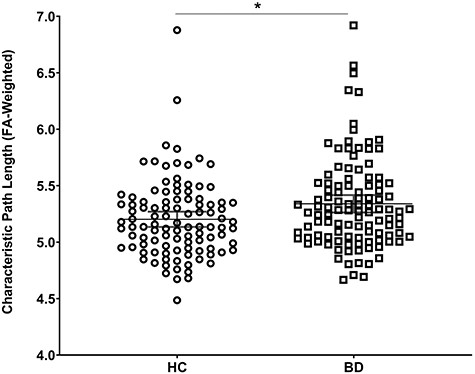
The BD group displayed longer characteristic path length compared with the HC group when connectivity matrices were weighted by the FA connection weight. Global connectivity was preserved when connected matrices were weighted by the NOS.
Subnetwork Analysis
Analysis of connected subnetwork components revealed group differences of the left frontotemporal component in BD compared with controls comprised of 13 nodes and 17 edges after FWER-correction (NOS-weighted matrices, P = 0.001) (Fig. 3). The statistically significant subnetwork included frontal inferior operculum, frontal inferior triangularis, rolandic operculum, insula, caudate, putamen, thalamus, hippocampus, Heschl’s gyrus, middle and superior temporal gyri, and pre- and postcentral gyri. The BD group showed greater dysconnectivity (NOS-weighted) in this subnetwork relative to the HC group.
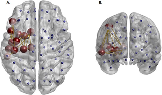
Red nodes reflect a subnetwork of brain regions with a significantly lower density (NOS-weighted) in the BD group compared with the HC group identified at T > 2. Blue nodes reflect the additional nonsignificant nodes defined by the AAL atlas. This left hemispheric component comprised of the frontal inferior operculum, frontal inferior triangularis, rolandic operculum, insula, caudate, putamen, thalamus, hippocampus, Heschl’s gyrus, middle and superior temporal gyri, and pre and post central gyri.
Normalized Rich-Club Coefficient
A normalized rich-club coefficient ϕnorm(k) was observed for NOS-weighted networks, with densities ranging from k13 to k30. A statistically significant difference between the BD and HC groups was observed in normalized rich-club coefficients across a range of densities, after multiple comparison correction at P < 0.001, where the BD group showed increased rich-club density relative to healthy controls (Fig. 4). A different slope in k appeared to be differentiated by research center when this was incorporated as a factor (Supplementary Fig. 1). Predictors were then added to the random model, where k appeared to have a direct effect on Ф. Site effects did not explain the observed diagnosis effect.
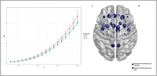
The graph presents the rich-club coefficient for Φ and k for BD and controls in NOS-weighted matrices. A normalized rich-club at k densities 13–30 was reported in this analysis. These findings withstand multiple comparison correction at P < 0.001 (BH corrected). One the right, rich-club structures differed between groups for the right middle frontal gyrus, and the left hippocampus at the statistically significant rich-club density threshold present among more than 60% of participants. These hubs were absent in the bipolar group rich-club network compared with controls.
Rich-Club Membership Differences between Patients and Controls
In NOS-weighted networks, rich-club membership was defined at the statistically significant network between patients and controls (P < 0.0001) for connections common to 60% or more of the participants. Nodes not involved in BD relative to controls rich-club membership were the right middle frontal gyrus and the left hippocampus (Fig. 4). Rich-club members were validated as the top 10% highest degree nodes within each diagnostic group.
Discussion
In this study, we applied graph theory metrics to a large multicenter diffusion MRI dataset and reported differences across metrics of integration in BD relative to controls. Patients with BD exhibited longer characteristic path length and reduced connectivity in a left frontotemporal network compared with controls. We also reported evidence for aberrant rich-club connectivity in BD, and frontal hub deficits in BD relative to controls. This study supports prior research that identified abnormal structural connectivity within cognitive and mood-regulating neuroanatomical circuits (Jeganathan et al. 2018; Roberts et al. 2018; Nabulsi et al. 2019).
At the whole-brain level, patients displayed longer paths and preserved global efficiency within their networks compared with controls. Path length can be largely influenced by longer paths in the network, whereas global efficiency is primarily influenced by shorter paths (Bullmore and Sporns 2009; Rubinov and Sporns 2010). This suggests that more long-range connections, as opposed to short-range connections, may be impaired and contribute to BD global dysconnectivity (Hagmann et al. 2010). A neurodevelopmental study in children and adolescents (aged 2–18 years old), reported a positive association between efficiency and age, not detected in path length, contributing to a model that these graph properties, whereas mathematically similar could describe different pathophysiological mechanisms related to development in long-range connections (Hagmann et al. 2010). Longitudinal network investigations are warranted to provide further insight into the progression of neural (dys)organization over time in BD.
We identified an impaired frontotemporal subnetwork, consistent with a prior focal tractography investigation using the present sample that identified reduced FA in the left anterior portion of the arcuate fasciculus in patients compared with healthy controls (Sarrazin et al. 2014). There are limited reports of impaired white matter connectivity within these inferior frontal cortices in BD (Versace et al. 2008; Kubicki et al. 2011; Hajek et al. 2013b; Emsell et al. 2014; Sarrazin et al. 2014). This may be due to the compact anatomical structure of the inferior frontal gyrus. A recent graph theory and subnetwork investigation identified impaired functional connectivity of the inferior frontal gyrus (Roberts et al. 2016). This study of young individuals with BD and their healthy relatives reported a similar dysconnected frontotemporal subnetwork as the present investigation, but with reductions in the right hemisphere (Roberts et al. 2016). Overlapping regions with the current study included the insula, inferior frontal gyrus, and rolandic operculum. The inferior frontal gyrus has been associated with appropriate attention, placing emotional meaning, and affect labeling (Hajek, et al. 2013a; Wegbreit et al. 2014). Few studies have investigated language deficits in mood disturbances, and the neurobiological role of the inferior frontal gyrus in BD has been controversial (Phillips and Swartz 2014). The current investigation observes both frontotemporal (Roberts et al. 2018) and basal ganglia and limbic (Nabulsi et al. 2019) anatomical dysconnectivity that have been observed previously in smaller samples. Reduced connectivity in subnetworks involved in language production, thought processing, and reward systems may represent more trait-like abnormalities in BD.
We observed increased connectivity between rich club regions in BD compared with controls, consistent with recent findings on smaller samples (Nabulsi et al. 2019; Zhang et al. 2019). This is in contrast to a number of studies that show preserved structural connectivity of the rich club in BD (Collin et al. 2016; Roberts et al. 2018; Wang et al. 2018). This inconsistency may be due to the absence of subcortical regions in the brain networks analyzed by Collin et al. (2016), despite their vital role in the pathophysiology of BD (Strakowski et al. 2012; Chase and Phillips 2016), different parcellation atlases employed as well as differing weightings applied to white matter connection estimates, namely unweighted (Roberts et al. 2018) and FA-weighted (Wang et al. 2018) in contrast to the weighting of streamline count in the present investigation. Differences seen with streamline count are consistent with streamline count weighted rich club connectivity differences reported in BD recently (Nabulsi et al. 2019).
Findings from this investigation and a prior investigation using similar methodology on an independent sample (O’Donoghue et al. 2017b) both reported impaired rightward frontal rich-club organization. These structural connectivity results are consistent with Crossley and colleagues’ findings, which indicate that functional over- and under- activations are more likely to be reported in rich-club hubs in psychotic illnesses (Crossley et al. 2015; O’Donoghue et al. 2017b). In the current investigation, impaired regional and subnetwork connections are consistent with the studies supporting impaired emotion and reward circuitries in BD. The findings also support leftward asymmetry of frontolimbic and frontal-striatal connectivity as a consistent marker of aberrant reward processing (Phillips and Swartz 2014).
Interestingly, studies indicate that voluntary behavioral control of positive and negative emotions includes specifically the right dorsolateral prefrontal cortex (DLPFC) and left ventrolateral prefrontal cortex (VLPFC), as these areas are involved in regulating emotional behaviors (Phillips et al. 2008). The findings of the current work converge with this hypothesis of an imbalance in left VLPFC and right DLPFC integration in BD. This was demonstrated in this study by differential right frontal rich-club organization and impaired subnetwork connectivity involving the left inferior frontal gyrus in subjects with BD relative to controls. These regions are involved in many regulatory processing and sensory networks, known to be functionally altered in BD. These network differences may suggest alternative pathways for communication within BD brains. For example, the overall increase in rich-club connectivity recorded in subjects with BD relative to controls may represent a compensatory mechanism to subnetwork dysconnectivity seen in patients. Our findings extend current models of BD pointing to a parallel rightward frontal and left-sided orbitofrontal-temporal network of dysconnected regions in BD. Understanding how a weakly connected left frontotemporal network and increased rich-club network underlie the pathophysiology of BD is complex and requires further study of structure–function relationships.
A major strength of the current investigation includes the large study population investigated. Although this study represents the largest investigation of structural networks ever conducted in BD, it is important to highlight that larger global efforts are warranted in BD to detect robust and generalizable factors that modulate disease progression and adequately model confounds and latent heterogeneity existing in patient groups. MR images were acquired on identical scanner models and acquisition sequence across research centers to reduce site-specific effects. Furthermore, this study utilized CSD during tractography reconstruction to account for the multiple fiber orientations within voxels. Recursive calibration corrected for partial volume effects when modeling the fiber orientation distribution (Jeurissen et al. 2014). This analysis employed standardized graph metrics allowing for comparability across graph theory investigations. A limitation of the current multicenter study was the differences in connection densities observed by research center due to differences in scanner hardware. Fortunately, the data were highly comparable, and there were no main effects due to scanner in statistically significant whole-brain measures of efficiency and path length. Of note, edge weights were not adjusted for tract volume, which can be dependent on voxel-size. In addition, we did not correct for region-of-interest volume, which can influence streamline count as it may be larger in some regions due to larger node size and therefore a greater number of projections tracking through those regions (de Reus and van den Heuvel 2013). It is important to note that beside group size and composition effects, other factors may influence the power of graph theory analyses to detect significant effects such as the choice of neuroanatomical atlas (Zalesky, Fornito, Harding, et al. 2010) and the model used to reconstruct white matter fibers (Calamante 2019), among many other factors. Thus, future studies should carefully consider these aspects when interpreting their results. Although an advantage of the current parcellation scheme included cortico-subcortical mapping, a subject-specific parcellation scheme would potentially confer increased anatomical accuracy. However, despite this limitation, the current study observes findings consistent with previous works that employ different schemes, which emphasize the reproducibility of the presented results, namely subnetwork and rich-club alterations in BD.
Furthermore, the lack of associations between the network abnormalities and clinical measures or medication use supports the presence of anatomical dysconnectivity as a trait-feature of BD, possibly related to genetic or developmental risk, or to associated features such cognitive dysfunction, which were not analyzed by the present study. Longitudinal designs and studies of at-risk subjects would help to clarify the clinical and functional implications of such connectivity abnormalities.
Conclusion
This study demonstrates anatomical dysconnectivity in BD, which is distributed beyond frontolimbic networks alone. A leftward predilection for impaired subnetwork connectivity, as well as increased rich-club connectivity, was identified in BD relative to controls. The application of graph theory to diffusion imaging data can identify abnormalities of large-scale and subnetworks associated with BD and help to elucidate the underlying neurobiology of the condition.
Notes
We would like to gratefully acknowledge the participants for taking part in this large research study. Conflict of Interest: The authors declare that there is no conflict of interest.
Funding
This study was supported by public funding from ANR MNP 2008 (grant to “VIP study”), the “Investissements d’Avenir” program ANR-11-IDEX-004-02 (Labex BioPsy) managed by the French Agence Nationale pour la Recherche and by the Fondation Pour la Recherche Médicale (“Bioinformatic analysis for research in biology” 2014 grant); by grants SFB636/C6 and We3638/3-1 from the German Deutsche Forschungsgemeinschaft; by grant R01 MH076971 from the National Institute of Mental Health.
L.N and G.M. research was supported by the Irish Research Council Postgraduate Scholarship. S.O. research was facilitated by the Hardiman Research Scholarship.
References
Author notes
Leila Nabulsi and Genevieve McPhilemy have contributed equally to this work.