


Abstract
Despite bariatric surgery being the most effective treatment for obesity, a proportion of subjects have suboptimal weight loss post-surgery. Therefore, it is necessary to understand the mechanisms behind the variance in weight loss and identify specific baseline biomarkers to predict optimal weight loss. Here, we employed functional magnetic resonance imaging (fMRI) with baseline whole-brain resting-state functional connectivity (RSFC) and a multivariate prediction framework integrating feature selection, feature transformation, and classification to prospectively identify obese patients that exhibited optimal weight loss at 6 months post-surgery. Siamese network, which is a multivariate machine learning method suitable for small sample analysis, and K-nearest neighbor (KNN) were cascaded as the classifier (Siamese-KNN). In the leave-one-out cross-validation, the Siamese-KNN achieved an accuracy of 83.78%, which was substantially higher than results from traditional classifiers. RSFC patterns contributing to the prediction consisted of brain networks related to salience, reward, self-referential, and cognitive processing. Further RSFC feature analysis indicated that the connection strength between frontal and parietal cortices was stronger in the optimal versus the suboptimal weight loss group. These findings show that specific RSFC patterns could be used as neuroimaging biomarkers to predict individual weight loss post-surgery and assist in personalized diagnosis for treatment of obesity.
Introduction
Bariatric surgery (BS) is the most effective treatment for obesity and related metabolic diseases (Gloy et al. 2013). Although significant weight loss typically results from BS (Sjostrom et al. 2004), a proportion of patients have suboptimal weight loss (Karlsson et al. 2007). The variability in the percentage of total weight loss (%TWL) ranges from 5% to 55% at 3 years post-surgery (Courcoulas et al. 2013). Therefore, it is important to understand the mechanisms behind the variance in weight loss and identify baseline biomarkers to predict optimal weight loss with BS.
Previous studies have identified that lower body mass index (BMI), larger waist circumference, younger age, and white race were associated with greater weight loss after BS (Carlin et al. 2008). However, investigators in the largest multicenter study on BS, the Longitudinal Assessment of Bariatric Surgery, examined the association between over 100 baseline variables and weight loss post-surgery, and results showed that few factors had significant predictive value (Courcoulas et al. 2015). Other studies also indicated that abnormal eating behavior (i.e., loss of control over eating) (White et al. 2010) and psychosocial factors (e.g., social support and psychiatric disorders) at baseline were not reliable predictors (Schrader et al. 1990; Herpertz et al. 2004). These reports concluded that these baseline behavioral measures were not effective predictors for future weight loss.
Growing evidence indicates that obesity is associated with impairment of executive control, reward evaluation, and homeostatic regulation of food intake, and these impairments are accompanied by disruptions of functional connections and brain networks that support cognitive control, reward, and homeostatic processing (Farr et al. 2016; Donofry et al. 2019; Li et al. 2020). For instance, obese individuals showed increased RSFC between regions involved in cognitive control (dorsolateral prefrontal cortex (DLPFC), medial prefrontal cortex (MPFC)), and reward processing (striatum) (Dietrich et al. 2016; Contreras-Rodriguez et al. 2017) and increased RSFC between region involved in homeostatic processing (hypothalamus) and regions involved in cognitive control and reward processing (Le et al. 2020a; Li et al. 2020; Lips et al. 2014). In addition, obesity is associated with disruptions of various resting-state networks including the default-mode network (DMN) (Tregellas et al. 2011; Kullmann et al. 2012), salience network (SN) (Garcia-Garcia et al. 2013; McFadden et al. 2013), frontoparietal network (FPN) (Ding et al. 2020), and basal ganglia network (BG) (Doornweerd et al. 2017). Specifically, DMN is thought to reflect a baseline state of brain function in which individuals are focused on their internal mental state. Disrupted RSFC strength within DMN in obese patients is associated with abnormal awareness of internal states such as appetite (Tregellas et al. 2011; Kullmann et al. 2012; Ding et al. 2020). SN is a paralimbic network that processes internal and external stimuli, including food stimuli and feeding behavior (McFadden et al. 2013). FPN is involved in inhibitory control in response to food cue. Increased functional network correlation between SN and FPN in obese patients is thought to reflect an imbalance between executive control and food stimulus processing (Ding et al. 2020). The abnormal RSFC strength in BG reflects the dysfunction of reward system and may result in higher intake of palatable high-fat foods (Doornweerd et al. 2017). In conclusion, RSFCs and brain networks play an important role in food intake and body weight regulation. BS is one of the most effective weight loss interventions for obesity, and it may work by ameliorating these aberrant patterns of network communication. In support, BS significantly decreased RSFC within the DMN comprising the anterior cingulate cortex (ACC), frontal superior gyrus, and orbitofrontal cortex (OFC) (Frank et al. 2014) and RSFC between insula and left precuneus (Lepping et al. 2015) and increased RSFC between hippocampus and insula and between posterior cingulate cortex (PCC) and DLPFC (Zhang et al. 2019). Although these studies have undoubtedly offered significant insights into brain RSFC abnormalities in obesity and BS-induced alterations, few studies have employed baseline brain RSFC to predict optimal post-surgery weight loss.
Recently, a growing number of studies using multivariate machine learning methods have demonstrated the capacity of RSFC in predicting treatment outcomes for major depressive disorder (Leaver et al. 2018), social anxiety (Whitfield-Gabrieli et al. 2016), epilepsy (Tomlinson et al. 2017), drug addiction (Steele et al. 2018), and behavioral lifestyle weight loss programs in obesity (Mokhtari et al. 2016; Mokhtari et al. 2018). Thus, these previous studies raise the possibility of using baseline RSFC to predict optimal weight loss after BS.
In contrast to group-level statistical methods, multivariate machine learning classification algorithms are capable of capturing complex multivariate discriminatory patterns in a way not possible using pairwise statistical analysis (Richiardi et al. 2013). Moreover, this methodology allows for personalized analyses where each participant can be classified rather than relying on group-level statistical outcomes (Plis et al. 2014; Mokhtari et al. 2018; Ju et al. 2019). Deep neural network methods have attracted interest in various fields including their use for the classification of brain disorders (Plis et al. 2014; Ju et al. 2019). However, a challenge for the application of deep neural network in neuroimaging classification or prediction is the overfitting problem since a large number of parameters need to be estimated in the deep neural network model while the number of samples for training is relatively small. Therefore, Siamese neural network (Chopra et al. 2005), which is a few-shot leaning method and has the ability to learn from few labeled samples, was introduced in the current study. During the training process of the Siamese network, the samples are pairwise fed into the network and the number of available training samples can be greatly augmented to avoid overfitting to some extent (Chu et al. 2018). Therefore, this method can be applied to classification problems where the number of training samples is small and hence is suitable for the current study.
Although weight loss after BS is a long-term process, previous studies have shown that the short-term weight loss after BS (i.e., 3 months and 6 months) was positively correlated with long-term weight loss (i.e., 12 months) (Nikolic et al. 2015) and was the strongest predictive factor of optimal weight loss up to 24 months post-surgery (Hindle et al. 2017). Here we selected weight loss at 6 months post-BS as the predicted variable and aimed to examine if baseline brain RSFC would be effective in predicting optimal post-surgical weight loss. We hypothesized that baseline brain RSFC patterns could serve as biomarkers for classifying obese patient with optimal and suboptimal weight loss at 6 months post-BS, and the associated RSFC patterns would be in key brain networks governing cognitive control, reward, self-referential processing, and saliency processing.
Materials and Methods
Participants
Forty obese patients were recruited for laparoscopic sleeve gastrectomy at Xijing Gastrointestinal Hospital affiliated to the Fourth Military Medical University in Xi’an, China. Patients with psychiatric or neurological diseases, previous intestinal surgery, inflammatory intestinal disease, organ dysfunction, or any current medication that could affect the brain were excluded. Obese patients had a waist circumference greater than the interior diameter of the scanner were also excluded (Li et al. 2018; Li et al. 2019b; Liu et al. 2019; Zhang et al. 2019; Zhang et al. 2016). Given the criteria, three individuals were disqualified for the magnetic resonance imaging (MRI) scan. Thus, 37 participants were used in this study. The experimental protocol was approved by the Institutional Review Board of Xijing Hospital and registered in the Chinese Clinical Trial Registry Center under number: ChiCTR-OOB-15006346 (http://www.chictr.org.cn). The study was conducted in accordance with the Declaration of Helsinki. All participants were informed of the nature of the research and provided written informed consent.
Participants underwent 12-hour overnight fasting, and MRI scans were performed at 9 AM to 10 AM. A trained clinician rated severity of subjects’ anxiety using the Hamilton Anxiety Rating Scale (HAMA) (Hamilton 1959) and depression using the Hamilton Depression Rating Scale (HAMD) (Hamilton 1960). All clinical measurements were identically conducted before (baseline, Pre) and 6 months after surgery (Post). Surgical procedures were performed by the same surgeon in all patients.
The sample set was split into suboptimal- (SOWL) and optimal-weight loss (OWL) groups by using the median of the percentage of total weight loss (%TWL) (Mokhtari et al. 2016; Mokhtari et al. 2018). The two-sample t-test was used to examine the difference between SOWL and OWL groups at baseline.
MRI Acquisition
The experiment was carried out using a 3.0-T Signa Excite HD (GE, Milwaukee, WI, USA) scanner. A standard head coil was used with foam padding to reduce head motion. Subjects were instructed to view a fixation cross and try to stay relaxed with their eyes open, not to think of anything particular during the scanning procedure.
First, a high-resolution structural image for each subject was acquired, using a three-dimensional magnetization-prepared rapid acquisition gradient-echo sequence with voxel size of 1 mm3 and with an axial fast spoiled gradient-echo sequence (TR = 7.8 ms, TE = 3.0 ms, matrix size = 256 × 256, field of view = 256 × 256 mm2, slice thickness = 1 mm and 166 slices). Then, a gradient-echo T2*-weighted echo planar imaging sequence was used for acquiring resting-state functional images with the following parameters: TR = 2000 ms, TE = 30 ms, matrix size = 64 × 64, FOV = 256 × 256 mm2, flip angle = 90 degrees, in-plane resolution of 4 mm2, slice thickness = 4 mm, and 32 axial slices. The scan for RS-fMRI lasted 360 s.
Image Processing
Imaging data were preprocessed using Statistical Parametric Mapping 12 (SPM12, https://www.fil.ion.ucl.ac.uk/spm/). The first five time points were removed to minimize nonequilibrium effects in the fMRI signal and then slice-timing and head movement correction were performed using default settings. In addition, head motion differences between the two groups were compared using the mean frame-wise displacement (FD) resulting from time derivatives of head translations and rotations (Power et al. 2012), and there was no significant group difference (P > 0.05) on mean FD (OWL, 0.19 ± 0.16 mm, SOWL, 0.22 ± 0.19 mm). Functional scans of each study participant were registered with the participant’s T1 structural scan and normalized (voxel size of 3 × 3 × 3 mm3) to the stereotactic space of the Montreal Neurological Institute (MNI) (Zhang et al. 2015b). Demeaning and detrending was performed, and time-varying head-motion parameters, white-matter signals, cerebrospinal-fluid signals, and global signals were regressed out as nuisance covariates (Power et al. 2014). fMRI time points that were severely affected by motion were removed using a “scrubbing method” (FD value > 0.5 mm, and root mean square variance of blood oxygenation level-dependent (BOLD) signal intensity, i.e., delta variation signal (DVARS) > 0.5% between consecutive time points) (Power et al. 2014), and <5% of time points were scrubbed per subject. Finally, band-pass temporal filtering (0.01–0.1 Hz) was used to remove effects of very low-frequency drift/high-frequency noise using REST toolkit (http://resting-fmri.sourceforge.net).
Resting-State Functional Connectivity Analysis
The functional MRI volumes were divided into 246 regions of interests (ROIs) according to the Brainnetome Atlas (Fan et al. 2016). Regional mean time series were obtained by averaging the fMRI time series in each ROI. Pearson correlation coefficients of time series between each ROI pair were calculated and normalized to Z scores using Fisher transformation, resulting in a 246 × 246 symmetric RSFC matrix for each subject. After removing 246 diagonal elements, the upper triangle elements of the RSFC matrix were extracted as features for subsequent analysis, and each subject had a feature vector with the dimension of 30 135 ((246 × 245)/2).
Outlier Removal
With a limited sample size, the data could be skewed due to the presence of outliers (Mohanty et al. 2018). Therefore, the median absolute deviation (MAD) (Leys et al. 2013) method was used to detect and remove features with outlier values (Mohanty et al. 2018). This method was performed for OWL and SOWL groups respectively. The features containing these outliers were eliminated, and only common retained features across the two groups were kept for further analysis (Supplementary Information-SI provides detailed information).
Feature Selection and Transformation
With regards to the small sample size for training compared to the dimensionality of feature vectors, an overfitting problem would occur if all RSFCs were used as features in a classifier. Therefore, it is necessary to conduct a feature selection step to retain only the most discriminating features and eliminate redundancy. First, a two-sample t test was applied to examine significant differences in RSFC between the two groups and a reduced number of RSFCs were retained by applying a statistical P threshold (Anderson et al. 2011). Then, the retained features obtained from the previous step were transformed to a lower-dimensional space using principal component analysis (PCA) (Jolliffe 1986) to eliminate correlations between features, and a set of orthogonal principal components (PCs) were extracted from the original dataset. Here all principle components were reserved and the constructed dimension-reduced subspace was only a change of the coordinate system without loss of information (Wang et al. 2012a).
Siamese-KNN classifier
The Siamese network comprises two identical neural networks and measures the similarity between the input paired samples through mapping input features into a target space where the sample distance (i.e., Euclidean distance) is small if two samples belong to the same category, otherwise the distance is large (Supplementary Figure S1). In our implementation, the subnetwork in the Siamese architecture was a four-layer back-propagation (BP) neural network (Fig. 1A) (Rumelhart et al. 1986). The number of neurons included in the input layer and two hidden layers were 36, 16, and 8 respectively, and the number of neurons in the output layer is 2. The hyperbolic tangent function (tanh) was adopted as the activation function in hidden layers. The loss function is
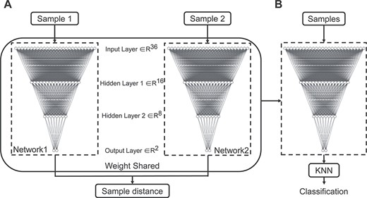
The Siamese network architecture and Siamese-KNN classifier. (A) The Siamese network architecture, which was made up of two BP networks with identical architecture and weights. The inputs to this network are two samples, and the output is the distance between two input samples in target space. (B) The Siamese-KNN classifier used in this study. The subnetwork in the trained Siamese network and KNN classifier was cascaded as the final classifier. Abbreviation: KNN, K-nearest neighbor.
|$1{r}_{decayed}=1{r}_{init}\times decay\_{rate}^{\big( global\_ step/ decay\_ step s\big)}$|where decay_rate was 0.9, decay_steps was 500, and the maximum iteration step was 10 000.
The Siamese network maps input features into a target space, but it does not classify samples. Thus, the simplest classifier K-nearest neighbor (KNN) (Cover 1967), which is a distance-based classifier, was employed to do the classification. When the Siamese network training was completed, subnetworks in the Siamese network and KNN classifier were cascaded as the final classifier (Siamese-KNN) (Fig. 1B) to predict the label of testing subjects. The Siamese network and KNN were implemented in python (version 3.5.6) using TensorFlow (version 1.10.0) and Scikit-learn library (version 0.21.3) (Pedregosa et al. 2011), respectively.
Prediction and Evaluation
The prediction framework integrating feature selection, feature transformation, and classification was adopted to predict optimal weight loss. As shown in Fig. 2, we implemented a leave-one-out cross validation (LOOCV) to estimate classifier performance as it provides an approximation of the test error with lower bias and is more suitable for a dataset with a small sample size (Mohanty et al. 2018). Specifically, for each LOOCV iteration, one subject was left out as testing subject and the remaining 36 subjects were used as training set. The above feature selection and transformation process was wrapped in the LOOCV to avoid overfitting. In the training step, the training set (n = 36) was used for feature selection and to train the feature transformation model. Then the training data and testing data were transformed to a new reduced feature space using the trained feature transformation model. The optimal P threshold in the feature selection was determined by a grid search (i.e., among 0.01 to 0.1 with stride 0.01). Then, the training data after the feature selection and transformation process were used to train the Siamese-KNN classifier. In the training of the Siamese network, we put subjects in the training set (n = 36) into 630 sample pairs |$\big({C}_{36}^2=630\big)$|, and the number of samples available for training was greatly augmented. In the testing step, the left-out subject for testing was evaluated with the trained classifier and the label of this sample was predicted. The above loop was repeated 37 times to predict the labels of all subjects. The accuracy, specificity, sensitivity, receiver operating characteristic (ROC) curve, and area under the ROC curve (AUC) were used to quantify the performance of the classifier.
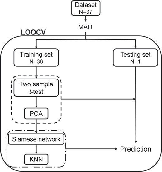
The leave-one-out cross-validation classification flowchart. MAD was employed to eliminate RSFC features with outlier values. On the training loop, the LOOCV split dataset into a training set and testing set. The training set was used for feature selection and transformation (the dash line), and to train the Siamese-KNN classifier (the dash-dotted line). Next, the built classifier was used to predict the label of the testing subject. After all loops, the average accuracy for all subjects was then calculated. Abbreviations: MAD, median absolute deviation; LOOCV, leave-one-out cross-validation; PCA, principal component analysis; KNN, K-nearest neighbor.
Significance Testing
A permutation test was conducted to estimate the statistical significance of the classification accuracy (Golland and Fischl 2003; Ojala and Garriga 2009). In the permutation test, the classification process was the same as the aforementioned step except for the samples’ label in the training set which was randomly permuted prior to training. The generalization rate (GR) is defined as the classification accuracy obtained by the classifier trained on the randomly re-labeled classification labels, and |${GR}_0$| is the classification accuracy obtained by the classifier trained on the real class labels. This permutation procedure was repeated 1000 times, and the number of times the GR was higher than the |${GR}_0$| which was recorded. A P value for the classification was then calculated by dividing this number by 1000 (Li et al. 2019a). The result was determined significant if P was < 5% (P < 0.05).
Consensus RSFCs
Since we applied a cross-validation strategy to predict subjects’ label, slightly different RSFCs were selected in each loop. By selecting the RSFCs that were repeatedly selected across all loops (i.e., with a 100% occurrence rate), we obtained the consensus RSFCs (Dosenbach et al. 2010; Jiang et al. 2018). For better interpretation and visualization, we grouped the 246 ROIs into 24 relatively larger brain regions (macroscale brain regions—MBRs) anatomically defined by the Brainnetome atlas (Fan et al. 2016; Jiang et al. 2018). Then, we counted the occurrence number of each MBR in the consensus functional connections. The importance of each MBR was evaluated according to its occurrence number in the consensus functional connections (Zeng et al. 2012).
Each PC represents a connectivity pattern. With regards to the limited sample size, only PCs with high consistency across LOOCV iterations were selected for subsequent analysis. The consistency was measured by the mean Pearson’s correlation coefficient between PCs in LOOCV iterations and corresponding PCs calculated from all the datasets. The strength of consensus RSFCs was also compared between two groups. The mechanisms of negative functional connectivity are still under debate (Fox et al. 2005; Murphy et al. 2009), and therefore, we focused on the functional connections which exhibited positive values (one sample t test, P < 0.01) (Wang et al. 2012b).
Comparison with Traditional Classifiers
In order to compare the performance of the Siamese-KNN classifier against traditional classification approaches, we performed a machine learning analysis using logistic regression (LR) (Tolles and Meurer 2016) and support vector machines (SVM) (Cortes and Vapnik 1995) with linear and radial basis function (RBF) kernel and BP neural network, respectively. The feature selection and feature transformation procedures were identical to the aforementioned analysis. The other two hyper-parameters (RBF kernel width |$\gamma$| and misclassification cost weight C) in SVM were fine-tuned by maximizing LOOCV accuracy via a grid search. The configuration of the BP neural network was the same as the subnetwork of the Siamese network implemented in the current study. Finally, the accuracy, specificity, sensitivity, and AUC were used as performance metrics and McNemar’s test was employed to compare the classification performance of Siamese-KNN with these four traditional classifiers (Everitt 1977; Dietterich 1998). The implementation of the LR and SVM classifiers was performed in Python using the Scikit-learn library (version 0.21.3) (Pedregosa et al. 2011), and BPNN was performed using Tensorflow (version 1.10.0).
Performance Evaluation of Different Network Configurations
To evaluate the effects of the number of hidden layers and neurons per layer on classification performance, we tried different numbers of hidden layers (i.e., among one to three hidden layers) and neurons (i.e., among 8, 16, 32) in each hidden layer. The performance of Siamese-KNN with different network configurations was evaluated through LOOCV.
Results
Demographic Characteristics
At baseline, there was substantial and statistically significant difference (P < 0.001, Table 1) in percentage of total weight loss between OWL and SOWL groups. There were no significant difference in gender, age, waist circumference, BMI, weight, HAMA, and HAMD based on group (P > 0.05, Table 1).
Demographic and clinical information, mean ± SE, on entire sample and the two weight loss groups
| Characteristics | Entire sample (N = 37) | OWL group (N = 19) | SOWL group (N = 18) | P |
|---|---|---|---|---|
| Age (years) | 27.35 ± 1.2 | 29 ± 1.65 | 25.61 ± 1.71 | 0.162a |
| Gender | 19M/18F | 8M/11F | 11M/7F | 0.248b |
| WC (cm) | 120.07 ± 1.84 | 118.97 ± 2.36 | 121.24 ± 3.04 | 0.558a |
| %TWL | 25.03 ± 0.91 | 29.13 ± 0.84 | 20.71 ± 0.84 | <0.001a |
| Baseline BMI (kg/m2) | 38.69 ± 0.67 | 38.42 ± 0.94 | 38.97 ± 0.99 | 0.686a |
| Baseline weight (kg) | 110.41 ± 2.77 | 107.14 ± 3.79 | 113.86 ± 4.00 | 0.230a |
| HAMA | 9.30 ± 0.89 | 9.32 ± 1.13 | 9.28 ± 1.41 | 0.983a |
| HAMD | 9.43 ± 0.98 | 9.53 ± 1.02 | 9.33 ± 1.33 | 0.923a |
Notes: aTwo-sample t-test.
bChi-square test.
Abbreviations: OWL, optimal weight loss; SOWL, suboptimal weight loss; WC, waist circumference; %TWL, percentage of total weight loss; BMI, body mass index; HAMA, Hamilton Anxiety Rating Scale; HAMD, Hamilton Depression Rating Scale.
Prediction Performance
In the LOOCV experiment, the Siamese-KNN achieved a classification accuracy of 83.78% (Supplementary Table S1), which was significantly higher than LR (64.86%, P = 0.016), SVM with linear (64.86%, P = 0.039) and RBF kernel function (67.56%, P = 0.031), but not significantly higher than the BP neural network (72.97%, P = 0.125) (Table 2). The ROC (Supplementary Figure S2) with an AUC of 0.84 indicated that the classifier developed here performed better compared to a random classifier. The P value revealed by the permutation test was < 0.001 (Supplementary Figure S3), suggesting that the classification results of the Siamese-KNN classifier were statistically significant. Different Siamese network configurations showed similar prediction performance (Supplementary Table S2), indicating its insensitivity to network configurations and robustness in small sample size classification.
The comparison of prediction performance between LR, SVM (linear kernel and RBF kernel), BP neural network, and Siamese-KNN
| Methods | |||||
|---|---|---|---|---|---|
| Metric | LR | SVM (linear) | SVM (RBF) | BPNN | Siamese-KNN |
| LOOCV accuracy | 64.86% | 64.86% | 67.56% | 72.79% | 83.78% |
| Sensitivity | 57.89% | 57.89% | 63.16% | 68.42% | 84.21% |
| Specificity | 72.22% | 72.22% | 72.22% | 77.78% | 83.33% |
| AUC | 0.73 | 0.72 | 0.68 | 0.77 | 0.84 |
| McNemar’s test (P) | 0.016 | 0.039 | 0.031 | 0.125 | — |
Note: Abbreviations: LR, logistic regression; SVM, support vector machine; RBF, radial basis function; BPNN, back-propagation neural network; KNN, K-nearest neighbor; LOOCV, leave-one-out cross-validation; AUC, area under the curve.
Consensus RSFC Analysis
After removing features with outlier values, 3892 out of 30 135 RSFCs were retained (Supplementary Figure S4). The hyper-parameter for P threshold in feature selection was determined by the grid search method and the optimal P threshold was 0.06. Since we applied a cross-validation strategy, slightly different RSFCs were selected by statistical feature selection method in each LOOCV iteration and there were 123 RSFCs (consensus RSFCs) selected across all iterations (Supplementary Figure S5). Then, we calculated the occurrence number of each MBR in the consensus RSFCs to evaluate the importance of each MBR (Supplementary Figure S6). Inferior parietal lobule, cingulate gyrus, lateral occipital cortex, superior frontal gyrus, and insula had the highest number of occurrences in the consensus RSFCs. Direct comparison of RSFCs strength showed that the consensus RSFCs between frontal and posterior parietal cortex were stronger (P < 0.05) in OWL group compared with SOWL group (Fig. 3).
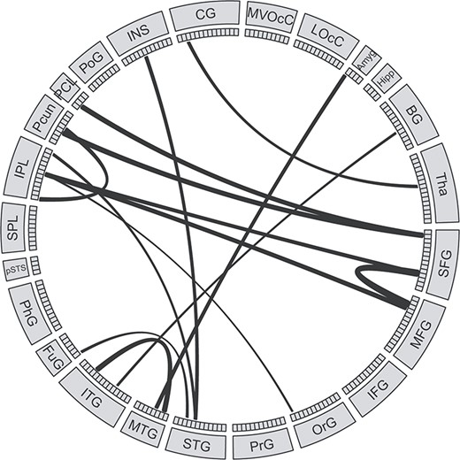
The consensus RSFCs that were stronger in the OWL than in the SOWL group. The size of the edges reflects the difference of RSFC strength between the OWL and the SOWL group.
Principal Components Representing Connectivity Patterns That Differ Between OWL and SOWL Groups
The PC1, PC2, and PC3 in each LOOCV iteration were highly correlated with the corresponding PCs calculated from the entire dataset (mean r value > 0.90, Supplementary Figure S7). Therefore, the first three PCs were consistent across each iteration with great generalization and stability. To provide a clearer visualization of the first three PCs, only 20 (~10%) connections with the highest principal component weight are shown in Fig. 4. The PC1 connectivity pattern represents a network dominated by interactions between regions including orbital gyrus (OFC), cingulate gyrus (PCC), basal ganglia (caudate), insula, and visual cortex (Fig. 4A). PC2 involves connectivity of the superior frontal gyrus (MPFC), cingulate gyrus (ACC, PCC), basal ganglia (caudate), and precuneus (Fig. 4B). PC3 represents a network that is dominated by connections between inferior parietal lobule (IPL), precuneus, cingulate gyrus (PCC), and postcentral gyrus (Fig. 4C). PC1 was negatively correlated with weight loss (Pre–Post, P < 0.001) and △BMI (Pre–Post, P < 0.001); PC2 was positively correlated with baseline weight (P = 0.001) and BMI (P = 0.010) (Fig. 5).
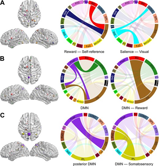
The connectivity patterns revealed by PCA. (A) PC1 connectivity pattern, (B) PC2 connectivity pattern, and (C) PC3 connectivity pattern. The size of each node in the left is directly related to its number of connections. Nodes from the same macroscale brain region are depicted in the same color. In the circular connectograms, the size of edges reflects the number of connections.
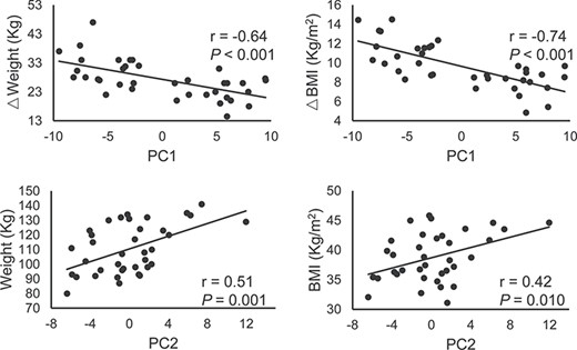
Correlation analysis between behavioral measurements and PCs. Abbreviations: PC, principal component; BMI, body mass index.
Discussion
Here we show that baseline RSFC patterns were able to classify obese patients with optimal and suboptimal weight loss at 6 months post BS with accuracy of 83.78% and AUC of 0.84. These findings corroborate our hypothesis that RSFC has potential to serve as a neuroimaging biomarker to help predict weight loss following BS. To the best of our knowledge, this is the first study to that has explored the potential for RSFC to serve as a biomarker for identifying obese patients with optimal weight loss post-surgery using a multivariate machine learning method.
With the relatively small sample size and large number of features, potential overfitting is a major challenge for the current study and most of other studies of the similar type. In order to avoid overfitting and ensure the generalization of the prediction model, feature selection (two-sample t test), and dimension reduction methods (PCA) were employed in the current study. Further, the Siamese network, which is a few-shot leaning method and has the ability to learn from few labeled samples, was employed for supervised feature transformation and resulted in a significantly higher classification accuracy of Siamese-KNN than LR and SVM. The accuracy of Siamese-KNN was not significantly higher than the BP neural network, which may be due to the small sample size. The excellent classification performance of the Siamese-KNN classifier in the current study showed its potential in clinical applications with small sample size.
Principal Components
As noted above, the prediction analyses combined PCA with machine learning methods identified patterns of multivariate connectivity that were effective in discriminating those who exhibited optimal weight loss after BS. The first three PCs with better generalization and stabilization contributed most to the classification performance. Each component represents a brain subnetwork that accounts for differences in connectivity between the two groups. It is worth noting that these network components cannot be dissected as individual brain regions or individual connections (Mokhtari et al. 2018). It is the entire connectivity pattern of the network component that was essential to prediction, in contrast to classical statistical approaches comparing one region at a time.
PC1 represents a network that is dominated by interactions between OFC, PCC, caudate, insula, and visual cortex, and weaker PC1 was associated with higher weight loss. OFC is an important region for assigning saliency value to food stimuli (including cues) and is implicated in compulsive food intake behaviors (Zhang et al. 2016). Increased activity of the OFC in obesity is associated with greater food reward sensitivity and significantly influences food intake behavior (Balodis et al. 2015). PCC is a midline cortical region implicated in self-referential processing (Northoff et al. 2006). Previous studies found that PCC activity was higher in obese/overweight compared to lean individuals (Kullmann et al. 2012) and that activity in this region was reduced following chronic exercise (Legget et al. 2016). The connection between OFC and PCC is associated with self-referential processes (Perrotin et al. 2015). The caudate modulates food reward processing, and the caudate response to the sight of calorie-predictive cues is higher in obese individuals compared to lean controls (Ng et al. 2011). The insular cortex, which also shows higher activity compared to lean control subjects in response to food cues (Scharmuller et al. 2012), is a multisensory region that serves as a nexus integrating interoceptive awareness, perception, emotion, and the processing of food visual stimuli (Frank et al. 2013). Prior work has demonstrated that visual imagery is a prime driver of food cravings (Kemps and Tiggemann 2010). Given this complex pattern, PC1 may represent the interactions between the regions from the reward (OFC, caudate), self-referential (PCC), salience (insula), and visual networks. These network interactions may play an important role in weight loss processes after BS.
PC2 was correlated with baseline weight and BMI and involves connectivity of MPFC, ACC, PCC, caudate, and precuneus, which are all core brain regions of the DMN. Activity in the DMN is thought to reflect a baseline state of brain function in which subjects are focused on their internal mental state. Several studies have reported that aberrant DMN activity may result in increased focusing on internal states or sensations such as appetite, food-related cognitive factors, or discomfort (Tregellas et al. 2011). Specifically, the MPFC is a core brain region in this network component and connects with many other brain regions. MPFC plays a critical role in emotional/behavioral functions that may affect appetitive behavior, and it is also a key brain region for value-based decision-making (Li et al. 2018) and reward-related behaviors (Vogt 2005). ACC is implicated in executive control of internal/external stimuli-related, context-dependent behaviors involving emotional information, and modulation of emotional response (Bush et al. 2000; Li et al. 2018). The abnormal activity of ACC may contribute to the imbalance between cognitive/emotional processing and increased risk to overeat (Kullmann et al. 2012; Meng et al. 2018). Precuneus and PCC play a critical role in self-referential processes and appetite control such as evaluating benefits of not eating compared with eating high-calorie foods (Yokum and Stice 2013). In obese individuals, the precuneus has greater activity at baseline (Zhang et al. 2015a) and higher functional connectivity to the DMN than lean adults (Kullmann et al. 2012). The caudate modulates reward processing and is implicated in various cognitive functions including inhibitory control (Dalley et al. 2011; Tschernegg et al. 2015) and goal-directed behavior (Balleine and O'Doherty 2010), and it has also been shown to play critical roles in ingestive behaviors (Nakamura and Ikuta 2017). The caudate-PCC/precuneus connectivity is associated with the success of body weight control (Nakamura and Ikuta 2017). Therefore, PC2 can be considered as a network that reflects the function of self-referential and executive control process, which may play an important role in body weight control.
PC3 is dominated by connections between IPL, precuneus, PCC, and postcentral gyrus. IPL, precuneus, and PCC are core components of the posterior DMN, which is involved in mostly unconscious processes that include self-representation, emotion, and salience detection (Knyazev 2012) as well as episodic memory quality (Ritchey and Cooper 2020). The postcentral gyrus is the primary somatosensory cortical area, involved in the integration of sensory stimuli with emotions, memory, and the body’s internal state (Aviram-Friedman et al. 2018). Therefore, PC3 may represent a network involved in unconscious processes of self-representation and somatosensory signals.
Consensus RSFC Analysis
During the cross-validation process, there were 123 consensus RSFCs selected across all loops for discriminating between individuals with optimal versus suboptimal weight loss. Comparing connection strengths between the two groups revealed that consensus RSFCs between the frontal cortex and parietal cortex were stronger in the OWL group than in the SOWL group. The frontoparietal control network regulates reward and cognitive functions associated with appetite and eating behavior (Park et al. 2016). Lower activation of frontoparietal brain regions implicated in inhibitory control may lead to greater sensitivity to the rewarding effects of highly palatable foods and disrupt the balance between reward processing and inhibitory control (Val-Laillet et al. 2015; Park et al. 2016). The subjective sense of loss of control over eating after BS has significant impact on weight loss outcomes, independent of the amount of food that is consumed (White et al. 2010). Therefore, the functional connection strength within the frontoparietal control network and the capacity for inhibitory control may influence weight loss post-surgery.
Limitation and Future Directions
Although this study has demonstrated that RSFC at baseline can be used to predict optimal weight loss, there are still several limitations. First, the study was constrained by the small sample size and the lack of an independent validation data set. Therefore, it is important to confirm the results using large multi-center datasets in the future. Second, the duration of resting-sate fMRI scan plays an important role in estimating RSFC. While many researchers use 5–7 min of resting-state data, as in the incurrent study (6 min), some investigators have found that the reliability and stability of RSFC estimates can be improved by increasing resting-state imaging duration (Birn et al. 2013). Therefore, it is important to replicate these results with longer resting-state BOLD sessions. Third, other imaging modalities including diffusion tensor imaging and T1-weighted imaging, peripheral hormones and clinical indices capturing complementary information could be included to improve the prediction performance. Fourth, the hypothalamus plays an important role in the regulation of eating behavior and body weight (Le et al. 2020a; Li et al. 2014; Zhang et al. 2020). The hypothalamus is not only the center of homeostatic control of eating, but it also communicates with multiple brain regions involved in reward (OFC, striatum) (Lips et al. 2014), interoception (posterior insula), motivation (thalamus), and inhibitory control (frontal and parietal cortices) (Le et al. 2020a) to determine food intake (Farr et al. 2016; Le et al. 2020b; Zhang et al. 2018). However, the hypothalamus was not included in the Brainnetome Atlas and some possibly important RSFCs of the hypothalamus are therefore not included in the classification scheme.
Conclusion
BS-induced weight loss varies among individuals, and differences in brain function between individuals are likely to influence long-term success in sustaining weight loss. Here we show that resting-state functional connectivity at baseline can be used to identify those obese patients with optimal weight loss after BS with classification accuracy of 83.78%. Connectivity patterns contributing to the prediction consisted of complex multivariate network components in brain networks associated with salience, reward, self-referential, and cognitive processing. Specifically, functional connections between the frontal cortex and parietal cortex were enhanced in the OWL group relative to the SOWL group, indicating that the strength of inhibitory control ability may influence weight loss after BS. These findings deepen our understanding of the underlying neurobiological mechanisms of variability in weight loss and demonstrate the feasibility of RSFC-based individualized prediction of optimal weight loss after BS.
Notes
Y.Z., G.J., and G.J.W.: study design; G.C. and Y. Han.: data collection; W.Z., G. Li., Y. Hu., J.W., Y. He., and G. Lv.: data analysis; W.Z.: drafting of the manuscript; K.V., Y.Z., P.M., D.T., G.J.W., and N.V.: critical revision of the manuscript. All authors critically reviewed the content and approved the final version for publication. Conflict of Interest: The authors declare no conflict of interest.
Funding
National Natural Science Foundation of China (Grant Nos. 61431013, 81730016, and 31670828); Open Funding Project of National Key Laboratory of Human Factors Engineering (Grant No. 6142222190103); National Clinical Research Center for Digestive Diseases, Xi’an, China (Grant No. 2015BAI13B07); Intramural Research Program of the United States National Institute on Alcoholism and Alcohol Abuse (Y1AA3009 to P.M., D.T., N.D.V., and G.J.W.).
References
Author notes
Wenchao Zhang and Gang Ji contributed equally to the work.