


Abstract
Functional connectivity (FC) matrices measure the regional interactions in the brain and have been widely used in neurological brain disease classification. A brain network, also named as connectome, could form a graph structure naturally, the nodes of which are brain regions and the edges are interregional connectivity. Thus, in this study, we proposed novel graph convolutional networks (GCNs) to extract efficient disease-related features from FC matrices. Considering the time-dependent nature of brain activity, we computed dynamic FC matrices with sliding windows and implemented a graph convolution–based LSTM (long short–term memory) layer to process dynamic graphs. Moreover, the demographics of patients were also used as additional outputs to guide the classification. In this paper, we proposed to utilize the demographic information as extra outputs and to share parameters among three networks predicting subject status, gender, and age, which serve as assistant tasks. We tested the performance of the proposed architecture in ADNI II dataset to classify Alzheimer’s disease patients from normal controls. The classification accuracy, sensitivity, and specificity reach 90.0%, 91.7%, and 88.6%, respectively, on ADNI II dataset.
Introduction
Neurological diseases, such as Alzheimer’s disease (AD) and major depression disease (MDD), cause abnormalities in brain functioning and affects patients’ daily lives. Functional MRI, which evaluates brain activity by measuring the blood oxygenation level-dependent (BOLD) over time, is thus a perfect tool to investigate possible brain functional changes in many neurological disorders. Considering the nature of functional integration and segregation in the brain, researchers assess the correlations among neuronal activities in order to analyze brain function. Resting state functional MR images are first segmented into several brain regions of interest (ROIs) according to a brain atlas, and the correlation between each pair of brain ROIs could be computed and summarized in a matrix, known as functional connectivity matrix.
Note that unlike natural images that contain shape and texture information, the spatial locality of the entries of FC does not directly correspond to the locality of brain networks. Thus, a difficult but important challenge in FC analysis is to extract efficient disease-related features. Reshaping FCs into vectors of features (Plis et al. 2014; Sen et al. 2016) and then sending it into off-the-shelf classifiers is a widely used operation. However, a vectorized FC will lose spatial information by discarding the topological structure of the matrix. Other feature extraction methods include BrainNetCNN (Kawahara et al. 2017), which proposed a cross-shape convolutional kernel to process connectivity matrix, as well as matrix clustering (Rajpoot et al. 2015).
A brain network can be represented as a graph structure naturally. It contains a set of brain regions of interest (ROIs), known as nodes, and describes their connectivity, known as edges. In the context of fMRI, the edges of brain functional graphs are derived from the correlations between each pair of brain ROIs. The nodes of brain functional graphs are the brain ROIs.
In brain network, graphical algorithms can be applied on FC data without loss of information. Graph kernel, which measures the inherent information in the graph structure (Vishwanathan et al. 2010; Shervashidze et al. 2011), is extensively used in many graph-based algorithms. Recently, researchers also applied graph kernel for neuro-imaging studies. For example, Jie et al. (Jie et al. 2014) used a graph kernel–based approach to measure directly the topological similarity between connectivity networks. However, the computational complexity of graph kernel is intensive.
Graph convolution neural networks (GCNs) allow an implementation of neural networks on graph structures. Neuroimaging pattern recognition applications include node classification and graph classification. Node classification assigns a predefined demographic graph for all subjects accompanied by a set of features. In the work of Parisot (Parisot et al. 2018), the feature of every individual, that is, every graph node, was a feature vector extracted from images, while the edges were calculated from the similarities between corresponding subjects. Graph classification treats each individual as an independent graph. For example, Ktena et al. (Ktena et al. 2018) proposed a Siamese graph convolution network to learn the similarity between brain networks. However, their works neglected the dynamic nature of brain activity, which can possibly improve the performance of classifiers.
Demographic information has been proved to be useful in many clinical studies. Researchers have reported a gender difference on cognitive functioning in brain (Halpern 2012). Besides, the incidence of many neurological diseases correlates with the years of age (Braak and Braak 1997; Butwicka and Gmitrowicz 2010). Thus, gender and age information was used in many neurological disease classification studies. However, in small datasets, which is common in medical imaging scenario, we argue that the status of subjects and demographic information of subjects are not always strongly correlated because of sampling preference. For example, a major guideline of collecting data for diagnosis is to balance the demographic distribution in both patient group and healthy control group, making gender and age weakly correlates with diagnosis. In this case, involving gender and age directly in the prediction model may not help models to learn diagnosis better.
In our previous work presented at a conference (Xing et al. 2019), a novel graph convolution recurrent network for fMRI pattern recognition was proposed. Graphs are defined with time-varying edges, that is, the dynamic functional connections, and fixed nodes, which are characterized by the structural information retrieved from average fMRI. The proposed method can improve diagnosis accuracy on fMRI through three aspects: 1) a graph classification algorithm which is dedicated for functional connectivity data; 2) an LSTM architecture that could further extract temporal information relevant to diagnosis; and 3) multitask settings that utilize demographic information as extra outputs for guiding the extraction of effective features. Details could be found in the following sections.
Materials and Method
We introduce below the proposed dynamic spectral GCNs with assistant task training using dynamic functional connectivity matrices, as in Figure 1. First, the dynamic connectivity matrices based on correlations of BOLD signals from sliding windows are defined as time-varying edges. Each node of the connectivity graph reflects an anatomical ROI. The feature on each node is defined by the volume of the corresponding ROI. Second, after defining the graph structure, a spectral graph convolution–based LSTM network is employed to extract information from the dynamic connectivity graphs. Finally, we make use of the demographic information as extra outputs, by adding two assistant networks with similar structure but different parameters, predicting gender and age. The feature maps from assistant networks were then weighted and combined with feature maps from the main network, guiding the parameter training and finally optimizing the results.
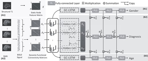
The schematic representation of the proposed DS-GCN with assistant task training for disease diagnosis using fMRI data. The static features of each node are defined by structural images (A1), and time-varying edges are defined by dynamic functional connectivity (A2). Dynamic graphs are then processed by diagnosis network (B2) and two subnetworks (B1 and B3) for assistance.
Graph Construction
A graph |$\mathcal{G}(\mathcal{V},\mathcal{E})$| was defined by two matrices, that is, node feature matrix and adjacency matrix. Node feature matrix denoted as|$X\in{R}^{M\times N}$|, where |$M$| is the number of nodes in the graph and |$N$| denotes the number of features, describes the property of every node in the graph. Node feature matrix describes the unique role of every node in the graph. Node feature matrix is required for graph convolutional operations and can be used as a check for graph isomorphism. If there are no node features provided, node feature matrix could be simply defined by identity matrix, where the numerical order of all nodes is binary encoded. Adjacency matrix |$A\in{R}^{M\times M}$| represents the graph structure in a matrix form.
As we do not have predefined node features for brain ROIs from fMRI data, we first choose the identity matrix as node feature matrix. To further differentiate the brain regions, we replaced the diagonal entry of identity matrix by the corresponding volume of each ROI. Thus, the feature matrix in our method is then denoted as
By aforementioned method, we could thus define a dynamic brain graph with static node features and dynamic connection pattern.
Graph Convolution LSTM
Graph Convolution
GC-LSTM
Dynamic graphs require a recurrent structure to handle temporal information. Recurrent structure is composed of a series of identical components, known as hidden cells. The output of each hidden cell is known as hidden representations. Hidden cells are aligned one after the other. By receiving the hidden representations learned in the last cell and outputting representations for following cell, dynamic graphs are processed in order. Hidden representations from all hidden cells are then sent into fully connected layers for the diagnosis result.
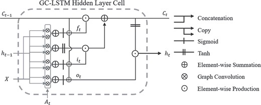
GC-LSTM hidden cell in detail. Each cell has two sources of input, the present (|${A}_t$| and|$X$|) and the recent past (|${h}_{t-1}$| and|${C}_{t-1}$|). Output sequence |$\{{h}_t|t=1,2,\dots T\}$| was then treated as feature maps for following layers.
Assistant Task Training
Gender and age provide important demographic information for disease prediction. Conventional deep learning classifiers added gender and age as additional features into the last fully connected layer. However, when adding demographic information as input features, the status and demographic information of subjects correlates in a statistical manner. For example, in ADNI datasets, gender and age are balanced among all groups, which makes these features correlate weakly with diagnosis labeling. In this situation, adding additional demographic features may not improve the classification performance. In addition, a balanced distribution in dataset does not imply a balanced distribution in real life: gender and age do affect the incidence of many neurological diseases (Hebert et al. 1995; Nebel et al. 2018). Thus, we propose to use demographic information as extra outputs in our networks. This strategy could not only improve the classification performance of weakly correlated demographic features but also guide the parameter optimizing in diagnosis task.
However, conventional multitask settings adopt a hard representation-sharing manner, by which different tasks share same parameters in beginning several convolutional layers of the network. In fact, it is difficult to decide which layers to be shared and which layers to be split among different tasks. Thus, our networks learn a linear combination of feature maps from different tasks to determine the shared representations by itself. We adopted this architecture from cross stitch networks (Misra et al. 2016), but our networks are task centralized, that is, only the main network, diagnosis network, receives the weighted combination of feature maps from assistant networks.
Experiments
We have compared the proposed method with a number of state-of-the-art classification approaches to demonstrate the improvements brought by graph convolution LSTM and assistant task training.
Data
We evaluated the proposed method on public dataset ADNI (http://adni.loni.usc.edu/) (Alzheimer’s Disease Neuroimaging Initiative). Under a series of criteria (http://adni.loni.usc.edu/wp-content/themes/freshnews-dev-v2/documents/clinical/ADNI-2_Protocol.pdf), ADNI-2 dataset is split into 177 healthy controls (HC), 191 early MCI (eMCI) patients, 158 late MCI (lMCI) patients, and 115 AD patients with 1.5 T T1-weighted structural images and functional images (subjects had their eyes open). From ADNI-2 dataset, we randomly chose 329 for training, 138 for validating, and 174 for testing. The model that performs best on validation dataset is chosen as the final model for testing. Data distributions of training, validating, and testing datasets are shown in Figure 3.
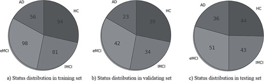
Demographic information of ADNI II dataset. The average age in training set is 73.6 years, average age in validating set is 73.7 years and 73.4 in testing set.
Preprocessing
Preprocessions of both structural and functional images are under a standard pipeline. The preprocessing steps of data is shown in Figure 4. For structural images, we performed anterior commissure (AC)—posterior commissure (PC) correction and then resampled them into size |$256\times 256\times 256$| with a resolution of|$1\times 1\times 1\ {\mathrm{mm}}^3$|. Then, after intensity inhomogeneity correction by N3 algorithm, structural images were skull stripped and registered into MNI space. Functional images were first slice time corrected by interpolation and motion corrected by a rigid body transformation on volumes, where mutual information was used as the cost function. Then, functional images were rigidly registered to the corresponding T1 MR images and further aligned to MNI space using the warping parameters of T1 MR to MNI space. Thus, functional images were demarcated into 116 ROIs by AAL (Automated Anatomical Labeling) template. Spatial filtering was applied with a Gaussian kernel with 4-mm FWHM (full width at half maximum). BOLD signals were then temporally filtered using a band-pass filter between 0.01 and 0.1 Hz. Dynamic functional connectivity matrices were computed by a sliding window after four nuisance covariates were regressed out, including head motion parameters, global mean signal, white matter signal, and cerebrospinal fluid (CSF) signal. Fisher-Z transformation was applied on all FC matrices.

Preprocessing steps of structural and functional data. Preprocessions of T1 images include AC-PC correction, resampling, intensity correction, skull stripping, and registration. Preprocessions of fMRI include slice time correction, motion correction, registration, spatial and temporal filtering, and nuisance covariates regression.
Ablation Study on Dynamic Graphs
In order to demonstrate the improvements brought by graph convolution LSTM, we compared the proposed method with several baseline models. We included 5 comparison methods in total, which compared two types of inputs, static FCs and dynamic FCs, as detailed below as well as shown in Figure 5. To ensure a fair comparison, all methods were trained under super parameters (i.e., learning rate, batch size, etc.), which could optimize their performances on validation set. We employed these methods on two different tasks: 1) HC versus AD, and 2)HC versus eMCI.
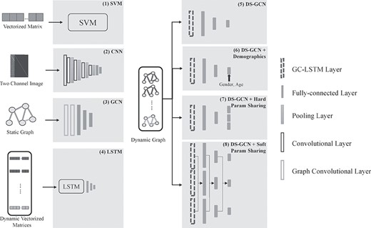
Schematic representations of all methods for ablation study. It should be noted that for every layer in our comparison, batch normalizations and ReLU activations were contained.
Static FCs. 1) SVM: Static FCs and brain ROI volumes were reshaped as vectors of features and were then put into SVM with Gaussian kernel. It should be noted that only entries in the upper triangle static FC matrices were used to reduce feature dimension. 2) CNN: Static FCs and node feature matrices were treated as two channel images and put into VGG-16. 3) GCN: Static graphs were constructed by static FCs and node feature matrix and then put into a graph convolution network with one graph convolution layer and three fully connected layers.
Dynamic FCs. 4) LSTM: Dynamic FCs were reshaped as a time series of features and then concatenated with static vectorized node feature matrices at every time point. 5) DS-GCN: No demographic information is used in this method. Dynamic graphs were constructed from functional connectivity matrices and structural information. The proposed network has one GC-LSTM layer followed by three fully connected layers. The detailed network layer dimensions are shown in Table 1.
Detailed network architecture of DS-GCN
| Layer | Input size | Output size |
|---|---|---|
| GC-LSTM | |$39\times 116\times 116$| | |$39\times 116\times 1$| |
| FL1 | |$39\times 116\times 1$| | |$116\times 1$| |
| FL2 | |$116\times 1$| | |$64\times 1$| |
| FL3 | |$64\times 1$| | |$2\times 1$| |
| Layer | Input size | Output size |
|---|---|---|
| GC-LSTM | |$39\times 116\times 116$| | |$39\times 116\times 1$| |
| FL1 | |$39\times 116\times 1$| | |$116\times 1$| |
| FL2 | |$116\times 1$| | |$64\times 1$| |
| FL3 | |$64\times 1$| | |$2\times 1$| |
Results. Classification results on ADNI II dataset are shown
Classification results of different algorithms on ADNI II dataset. The classification task is to classify HC and AD
| Inputs | Methods | Accuracy | Sensitivity | Specificity |
|---|---|---|---|---|
| Static FCs | SVM (linear kernel) | 68.8% | 72.2% | 65.9% |
| Spectral GCN | 81.3% | 88.9% | 75.0% | |
| CNN | / | / | / | |
| Dynamic FCs | LSTM | 78.8% | 86.1% | 72.7% |
| DS-GCN | 83.8% | 80.6% | 86.4% |
| Inputs | Methods | Accuracy | Sensitivity | Specificity |
|---|---|---|---|---|
| Static FCs | SVM (linear kernel) | 68.8% | 72.2% | 65.9% |
| Spectral GCN | 81.3% | 88.9% | 75.0% | |
| CNN | / | / | / | |
| Dynamic FCs | LSTM | 78.8% | 86.1% | 72.7% |
| DS-GCN | 83.8% | 80.6% | 86.4% |
in Tables 2 and 3. From the tables, one can observe that overall graph-based networks performed better than no graph–based methods. In addition, dynamic connectivity outperformed static connectivity methods. The results indicate that dynamic connectivity with graph-based neural networks could fully exploit the information in fMRI connectivity analysis.
Classification results of different algorithms on ADNI II dataset. The classification task is to classify HC and eMCI
| Inputs | Methods | Accuracy | Sensitivity | Specificity |
|---|---|---|---|---|
| Static FCs | SVM (linear kernel) | 60.0% | 80.4% | 38.6% |
| GCN | 70.5% | 76.4% | 63.6% | |
| CNN | / | / | / | |
| Dynamic FCs | LSTM | 67.3% | 64.7% | 70.5% |
| DS-GCN | 71.6% | 68.6% | 75.0% |
| Inputs | Methods | Accuracy | Sensitivity | Specificity |
|---|---|---|---|---|
| Static FCs | SVM (linear kernel) | 60.0% | 80.4% | 38.6% |
| GCN | 70.5% | 76.4% | 63.6% | |
| CNN | / | / | / | |
| Dynamic FCs | LSTM | 67.3% | 64.7% | 70.5% |
| DS-GCN | 71.6% | 68.6% | 75.0% |
Ablation Study on Assistant Task Training
To demonstrate the efficacy of assistant task training, we employed the strategy on several deep learning–based models, including GCN, LSTM, and DS-GCN. The results can be seen in Table 4.
Classification results under different settings on ADNI II dataset. The classification task is to classify HC and AD
| Models | Settings | Accuracy | Sensitivity | Specificity |
|---|---|---|---|---|
| GCN | Naive | 81.3% | 88.9% | 75.0% |
| Extra input | 80.0% | 83.3% | 77.3% | |
| Hard parameter sharing | 83.8% | 83.3% | 84.1% | |
| Soft parameter sharing | 83.8% | 86.1% | 81.2% | |
| LSTM | Naive | 78.8% | 86.1% | 72.7% |
| Extra input | 80.0% | 80.6% | 79.5% | |
| Hard parameter sharing | 81.3% | 77.8% | 84.1% | |
| Soft parameter sharing | 85.0% | 80.6% | 88.6% | |
| DS-GCN | Naive | 83.8% | 80.6% | 86.4% |
| Extra input | 86.3% | 88.9% | 84.1% | |
| Hard parameter sharing | 87.5% | 91.7% | 81.8% | |
| Soft parameter sharing | 90.0% | 91.7% | 88.6% |
We compared assistant task learning strategy with other multitask settings. 1) Demographic input: In this method, demographic information, that is, gender and age, was used as extra inputs in the last fully connected layer. 2) Hard parameter sharing: We compared hard parameter sharing, where different tasks share the same parameters in front layers of the network with the proposed algorithm. Networks were split for three tasks at the last fully connected layer. 3) Soft parameter sharing: Soft parameter sharing is the proposed method and the feature maps from assistant networks were weighted and combined with feature maps from main network.
When we compared different settings of our algorithm, the performance by using assistant task training outperformed those without such a training strategy. Assistant task training may help improve the performance of classification.
Multilabel Classification Tasks
Despite of binary classification tasks, we also tested the proposed method under multilabel setting, as in Table 5. The outputs of the model are a 4-channel one-hot encoded labels representing HC, eMCI, lMCI, and AD, respectively. Recall (sensitivity), precision, and F1-score are the mostly used evaluation metrics for multilabel classification tasks. Recall is the fraction of the total amount of instances, which were correctly selected. Precision is the fraction of correctly selected cases of one class among all cases that were classified as this class. F1-score is the harmonic means of recall and precision.
Classification results of multilabel classification tasks. The classification task is to classify HC, eMCI, lMCI, and AD
| Class | Sensitivity (recall) | Precision | F1-score |
|---|---|---|---|
| HC | 65.9% | 60.4% | 63.0% |
| eMCI | 70.6% | 65.4% | 67.9% |
| lMCI | 63.9% | 52.3% | 57.5% |
| AD | 62.8% | 100.0% | 77.1% |
| Avg | 65.8% | 69.5% | 67.6% |
| Class | Sensitivity (recall) | Precision | F1-score |
|---|---|---|---|
| HC | 65.9% | 60.4% | 63.0% |
| eMCI | 70.6% | 65.4% | 67.9% |
| lMCI | 63.9% | 52.3% | 57.5% |
| AD | 62.8% | 100.0% | 77.1% |
| Avg | 65.8% | 69.5% | 67.6% |
Discussion
To further demonstrate the improvements in our model and to evaluate the assistant task training strategy, we compared the computational cost of all methods for comparison, computed the class activation map of our model, and plotted the contribution from assistant tasks during training. The proposed model consumes less storage and operations than other methods and located bilateral hippocampus, right precuneus, right frontal middle cortex, and left precentral cortex as class activated brain regions. Feature maps from gender and age prediction tasks have shown increasing contributions to diagnosis task through training.
Computational Cost
We compared the FLOPs (floating point operations) (Hunger 2005) and the physical size of aforementioned models. Comparing to the baseline models without using demographic information, the learnable parameters are tripled in our methods with soft parameter sharing. Besides, to handle dynamic FC, we implemented LSTM structure into our network, also causing a considerable increase of parameter amount.
However, as shown in Table 6, even with three times larger than baseline DS-GCN, the proposed method still consume less storage and operations than state-of-the-art methods, such as SVM, CNN, and LSTM. We attribute it to the computational simplicity of GCN. Considering an adjacency matrix|${A}^{116\times 116}$| and a node feature matrix|${X}^{116\times 116}$| and vectorizing both matrices as input, SVM requires at least 6670 (upper triangle entries in connectivity matrix) + 116 (diagonal features) parameters to assign a prediction. However, if we adopt graph convolution as described in equation (5), the dimensionality of parameters needed declines into 116 × 1. Graph convolution allows matrix calculation on functional connectivity matrices and thus considerably reduce the number of parameters. It is also worth noting that in GCN model, we implemented two graph convolution layers to ensure a stable and acceptable performance, making GCN model more complex than DS-GCN.
Parameter sizes of different models. For ADNI-2 dataset, |$T=39$|
| Methods | Input resolution | Size/kiB | FLOPs/kMAC |
|---|---|---|---|
| SVM (linear kernel) | |$6786\times 1\times 1$| | 18.4 × 10² | 13.2 |
| GCN | |$116\times 116\times 1$| | 64.4 | 22.2 |
| CNN | |$116\times 116\times 2$| | 12.2 × 10³ | 14.5 × 10⁶ |
| LSTM | |$13572\times 1\times T$| | 52.5 × 10⁵ | 9.3 × 10⁴ |
| DS-GCN | |$116\times 116\times T$| | 39.5 | 21.0 |
| DS-GCN with demographics | |$116\times 116\times T+2$| | 39.5 | 21.0 |
| DS-GCN with multi-task | |$116\times 116\times T$| | 41.1 | 21.1 |
| DS-GCN with assistant task training | |$116\times 116\times T$| | 121.7 | 72.1 |
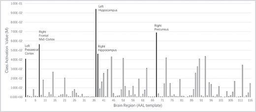
A bar chart showing the average class activation value of all test subjects. Top 5 activated regions are shown in different colors. Left hippocampus is reported as the most active region when our model diagnosis AD.
Network Explainability
The class activation map |$\mathrm{M}$| is the feature map |${x}_D^1$| filtered by importance weight:
|${\mathrm{M}}_{\mathrm{c}}= ReLU({\omega}_c{x}_D^1).$| Here, activation function ReLU makes heat map focus on brain regions, which only play positive parts in classification. The class activation value of all testing subjects is averaged and shown in Figures 6 and 7.
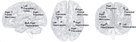
The Alzheimer’s disease activation map shown on a smoothed MNI 152 template. This image is shown by BrainNetViewer (Xia et al. 2013).
Analysis on Assistant Task Training
Synthetic Experiment
To illustrate the effectiveness of assistant task learning, we reproduced the result of a synthetic experiment from (Caruana and Sa 1997). Here, we used two fully connected layer with activation function to approximate|${(A+B)}^2$|. |$A$| and|$B$| are uniformly chosen from range |$[-5,5]$| and are encoded into |${2}^{10}$| bins. Besides the binary codes of |$A$| and|$B$|, another feature |${(A-B)}^2$| is also provided. However, |${(A-B)}^2$| weakly correlates with our target (the correlation reaches zero if |$A$| and|$B$| are “random” enough). This does not mean we should discard|${(A-B)}^2$|. By using |${(A-B)}^2$| as extra outputs, our simple network could easily generate the best prediction performance by learning to model subfeatures |$A$| and|$B$|. Figures 8 and 9 show the network design and the result of this synthetic experiment.
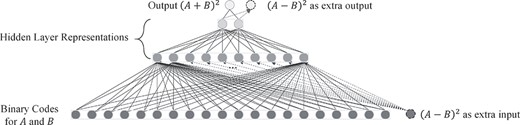
Network design for synthetic experiment to illustrate the effectiveness of assistant task learning. The classification model is composed of three fully connected layers. Number of node here represents the dimension of features.

The result for synthetic experiments. Both |${(A-B)}^2$| and |${(A+B)}^2$| are normalized. The mean squared error for prediction without |${(A-B)}^2$| (naive) is 0.016. The mean squared error for prediction with |${(A-B)}^2$| as an extra input is 0.036 and is 0.009 for prediction with |${(A-B)}^2$| as an additional output.
Task Contribution
The numeric values of |$\alpha$|s as well as the values of losses during training are plotted in Figure 10. To present the stable contribution from different tasks, we compared the updating values of alphas under different initializations. Experiment results show that using the training part of ADNI dataset, from which 43 subjects (20% of the training dataset) was selected for validation. Training procedure in all experiments used Adam (Kingma and Ba 2015) with initial learning rate|${10}^{-3}$|. For random initialization, the cross entropy loss of diagnosis and gender classification were between [0.6, 0.8], while the MSE loss of age prediction were between [0.07, 0.08]. Thus, to weight the losses from different tasks into the same scale, the weights of losses were then |${\omega}_D={\omega}_G=1,\ {\rm and}\ {\omega}_A=10$|. As seen in equation (6), |${\alpha}_D$| refers to the weight of the main tasks, |${\alpha}_G$| refers to the contribution from gender, and |${\alpha}_A$| refers to the contribution from age. These values reflect the influences of each factor to the final classification performance.
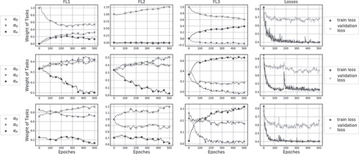
Alpha values of different layers under different initializations. Assistant task training shown in the first row was initialized with |${\alpha}_D=1$| and|${\alpha}_G={\alpha}_A=0$|, while in the second row was initialized with|${\alpha}_D={\alpha}_G={\alpha}_A=0.33$|. Figures of the third row show alpha values randomly initialized.
The above results confirmed our hypothesis that the training of gender classification and age prediction may help generate stable and robust network feature maps for diagnosis task. Alphas in the last convolutional layers did not change as dramatically as the first two layers, indicating a weaker correlation among different tasks for deeper layers.
Conclusion
In this paper, we have proposed a model specially to deal with dynamic functional connectivity. The novelty of this paper can be shown in three aspects. First, we proposed a specially designed graph construction algorithm, which could utilize both functional and structural MR images; second, a spectral graph convolution–based recurrent network is implemented to extract both functional and spatial information; and last, our model adopts a training strategy, which utilizes demographic features as extra outputs, guiding the diagnosis network to train and focus. Our work provides not only a new and efficient way to analyze functional MR images but also a new perspective for the usage of semantic features.
However, there were still some limitations in our study. First, we used AAL atlas to demarcate the brain into 116 brain ROIs. Although there exist several brain atlases, such as automatic nonlinear imaging matching and anatomical labeling (ANIMAL) (Collins and Evans 1999), and Talariach Daemon (TT) (Lancaster et al. 2000), AAL atlas is most widely adopted in fMRI studies and also chosen as default template in SPM software. However, the choice of brain nodes could affect the result of functional connectivity networks. In this work, we proposed graph LSTM, which is a general method and could also be used in different brain atlas settings. Second, we only used volume as our structural node features because it is easily obtained and the volume is highly related with the onset of AD (Bartos et al. 2019; Zhao et al. 2019). However, we do not test the algorithms with more other structural features including cortex thickness and image intensity.
Data Availability
The dataset used in this work (ADNII) is an open-source dataset downloaded from http://adni.loni.usc.edu/.
Notes
This work was supported in part by the National Natural Science Foundation of China under Grant 81830056, Shanghai Health System Excellent Talent Training Program (Excellent Subject Leader) 2017BR054 and Shanghai Municipal Education Commission-Gaofeng Clinical Medicine Grant Support, 20172029. Conflict of interest: X.X, Q.L, H.W. are interns, and Z.X. and F.S. are employees of Shanghai United Imaging Intelligence Co., Ltd. The company has no role in designing and performing the surveillances and analyzing and interpreting the data. All other authors report no conflicts of interest relevant to this article.
References
Author notes
Xiaodan Xing and Qingfeng Li have contributed equally to this work.