


Abstract
The Southwest Maluku region in eastern Indonesia is considered a frontier, outermost and underdeveloped region. Its inhabitants live on isolated islands, including the residents of Mahaleta Village, where only 9.4% of the community have limited access to electricity. This study aimed to design an economically feasible hybrid renewable energy (RE) system based on solar and wind energy to integrate with the productive activities of the village. The study developed conceptual schemes to meet the demand for electricity from the residential, community, commercial and productive sectors of the village. The analysis was performed using a techno-economic approach. The hybrid system was designed using the HOMER Pro optimization function, and cold-storage and dryer systems were designed to support related productive activities. The optimized design of the hybrid RE system comprised 271.62 kW of solar photovoltaics, 80 kW of wind turbines and a 1-MWh lead–acid battery. We found that the hybrid RE system would only be economically feasible with a full-grant incentive and an electricity tariff of $0.0808/kWh. However, the productive activity schemes were all economically feasible, with a cold-storage cost of $0.035/kg and a drying cost of $0.082/kg. Integrating the hybrid RE system with productive activities can improve the economic feasibility of the energy system and create more jobs as well as increase income for the local community.
Introduction
Access to energy and electricity drives economic development and plays an important role in increasing the productivity of communities. Hence, better access to energy and electricity contributes to alleviating poverty by providing poor people with more productive opportunities [1]. Underdeveloped regions are areas, usually within a province, that are relatively less development compared with other regions on a national scale based on several criteria, such as economic conditions, human capital, infrastructure, local government budget, geographic location, accessibility and susceptibility to disasters and conflict [2, 3]. In Indonesia, these regions are also known as frontier, outermost and underdeveloped (terdepan, terluar, tertinggal, or the 3T) regions. The 3T regions are concentrated in isolated parts of Indonesia, which have low accessibility and are located far from the centre of growth [2], preventing the development of economic and human resources in these regions.
In remote rural areas, access to electricity can stimulate economic growth through improved household income and higher purchasing power, a higher employment rate and improved productivity [4]. However, people living in isolated areas have difficulty accessing electricity due to infrastructural and economic factors. These challenges are inevitably encountered in archipelagic countries such as Indonesia, where the population distribution is spread throughout the country and electricity is mainly sourced from centralized power plants [5]. The complexity of the infrastructure and poor access to remote areas due to geographical conditions make it difficult to extend the main grid connections to remote rural areas [6]. Therefore, the provision of electricity in remote rural areas is more expensive [7].
On the other hand, underdeveloped rural regions tend to have small populations with a low income level, which leads to low electricity demand in these regions [7, 8]. As income level is proportional to affordability, residents of underdeveloped rural regions typically have low access to affordable electricity [7]. These factors contribute to the disinterest of private power companies in investing in rural electrification projects due to limited financing options [8].
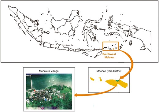
Eastern Indonesia is one of the regions in Indonesia that still has provinces with an electrification ratio of <95%; for example, the province of Maluku has an electrification ratio of 93% [9]. Maluku comprises several islands surrounded by the deep Banda Sea, which has great natural resources and energy potential [10]. The solar and wind energy resources of the province are relatively abundant compared with the average resources in Indonesia. Several districts in Maluku are considered 3T regions, such as Southwest Maluku [11]. Compared with Indonesia’s gross domestic product (GDP) of $4784 per capita [12], Southwest Maluku had a relatively low GDP of $1549 per capita in 2022 [13]. Southwest Maluku is located 494.55 nautical miles south of the main island of the province [14], roughly a 3-day sea voyage away. The district comprises 48 small islands and 88.1% of its area is water [14]. Fig. 2 illustrates the location of the region. The geographical characteristics and the fact that rural settlements are unevenly distributed in remote areas make providing electricity there very challenging.
Analysis framework
Residents of border regions have reported much lower energy accessibility than people living on the other side of the national border [15]. Southwest Maluku is directly adjacent to two countries: East Timor and Australia. Hence, the availability of energy, especially electricity, in this region would not only support socio-economic development, but also strengthen national security [16]. Furthermore, the availability of energy in border regions would decrease the economic disparity between residents of the border region and others. Consequently, residents are becoming unlikely to move to one of the neighbouring countries.
To increase the availability of electricity in remote rural areas, the National Electricity Supply Business Plan (RUPTL) describes the strategy of the state-owned electricity company, Perusahaan Listrik Negara (PLN), of deploying power plants that would utilize locally sourced renewable energy (RE) [17]. A small-scale decentralized energy system has been deemed an effective solution to provide electricity service to rural communities on remote islands [18, 19]. The implementation of a hybrid renewable energy system (HRES) is common in isolated areas because the HRES combines RE generation technologies and can operate in stand-alone mode [20]. Incorporating hybrid technologies into RE systems can address the constraints that may be induced when the system uses intermittent RE, such as efficiency and reliability [20]. Using renewables to power rural electrification can also tackle climate change issues by contributing to increasing the share of RE in Indonesia’s energy mix [21]. Rural electrification can also trigger local development through the ability to use the generated electricity in productive sectors [22]. Moreover, private entities can own and operate certain decentralized RE technologies such as solar photovoltaics (PV) on a small scale [23]. Therefore, applying HRES in rural areas to enable electricity access could create new job opportunities and boost the economic growth of local communities [24].
Various studies have been conducted on hybrid power generation systems in remote rural areas. Das et al. [25] evaluated the levelized cost of electricity (LCOE) and life-cycle emissions associated with the HRES to fulfil residential, commercial and community electricity demands on a remote Bangladeshi island. Murugaperumal et al. [26] designed a system based on the estimated electrical load of an Indian village’s residential, commercial, institutional and agricultural sectors. Ahmad et al. [27] analysed the feasibility of applying HRES to enable electricity sales during low demand and found that a hybrid grid-connected system had a lower cost of electricity (COE) than an off-grid system. Barzola et al. [28] examined the impact of the subsidized and unsubsidized diesel price on the HRES COE in a rural settlement in Ecuador. Ramesh and Saini [29] found that discount rates, battery cost and variation in PV costs significantly impacted the HRES in rural India. Hardjono et al. [30] found that a minimum grant of 25% was required for the feasibility of long-term planning of energy system integration with productive zone development on an isolated Indonesian island. Putro and Purwanto [31] clustered Indonesia’s 3T villages and found that the combination of tax allowances, interest subsidies, grants and carbon emission reduction made microgrids viable in those village clusters.
The studies mentioned above conducted technical and economic analyses of hybrid renewable power generation systems. However, the analyses [25–29] were limited to the COE of the system, and some studies designed an energy system capable only of meeting the electricity demand in existing non-productive and productive sectors in specific remote rural settings. To fill the research gap, this study expands the scope to Indonesia’s isolated regions [30, 31] by designing an HRES that can support the development of new productive sectors based on the socio-economic potential of the region, thus prospectively improving the economic feasibility of the system. This study also includes the electricity tariff and compares it to the purchasing power of residents of the remote rural area of interest in eastern Indonesia.
This study aims to design an economically feasible PV–wind HRES capable of meeting the demand for electricity from the residential, community and commercial sectors, and evaluate the integration of productive economic activities into the HRES. Productive sector development is expected to be an enabler in maximizing the value of Mahaleta Village’s natural resource potential, which may increase the community’s productivity and welfare. Additionally, an HRES can help accelerate infrastructural development in Southwest Maluku and support the achievement of Indonesia’s electrification ratio and RE mix goals. The research results are believed to be relevant and potentially applicable to other underdeveloped rural areas facing similar problems.
1 Methodology
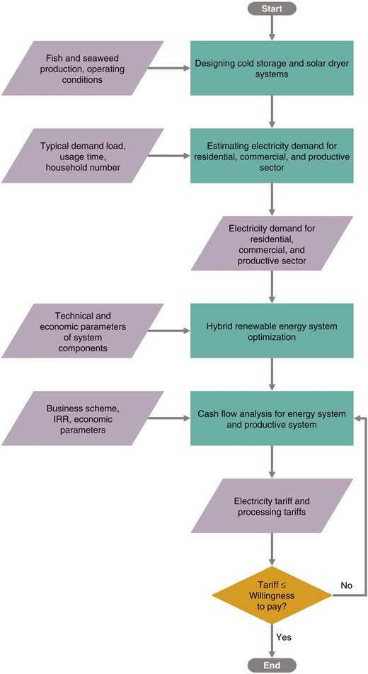
This study was carried out according to the analysis framework shown in Fig. 1.
1.2 Study area
Southwest Maluku has 17 subdistricts, 10 of which have not been electrified by the state-owned electricity company, PLN. Among them is the subdistrict of Mdona Hyera [32], where three villages still do not have access to electricity. Mahaleta Village (Fig. 2) is one of these and therefore was suitable as the research setting for this study. Mahaleta was selected as a case for examining the integration of an HRES with productive activities in underdeveloped rural areas. Its geographic coordinates are 8° 11’ 18.751” S and 128° 56’ 3.318” E, and its area is 24.52 km2. The village population is ~344 and the population density is 14.03 per km2 [32].
Ninety-six families live in Mahaleta on the main island of Mdona Hyera. Most villagers work in the plantation sector and are also involved in fishery activities such as catching and cultivation [32]. The region has an abundant fish and seaweed cultivation potential with a high economic value [33]. For example, fish and seaweed production reached 13 550 tons in 2020 [32]. However, the sector is still run on a small scale using conventional methods. One of the reasons for this is the lack of processing facilities due to a limited electricity infrastructure, which results in low commodity economic added value and limited market reach to distribute marine produce. Currently, only 9.4% of the village population has access to electricity through an independently owned diesel generator used exclusively for nocturnal activities [32]. Limited electricity as a consequence of high fuel prices due to the remoteness of the region means that the village does not yet have adequate facilities to maximize its resource potential. Therefore, this study proposes the use of an HRES to generate electricity and encourage the socio-economic development of the village.
1.3 Supply resources
1.3.1 Solar irradiation
Solar radiation data for Mahaleta were retrieved from the RenewablesNinja website [34–36] that uses the database from National Aeronautics and Space Administration (NASA) MERRA [37] and the Satellite Application Facility on Climate Monitoring (CM-SAF) SARAH data set [38, 39] for the year 2019 and are depicted in Fig. 3a. As shown, solar radiation ranges from 3.7 to 7.2 kWh/m2/day, with an annual average of 5.64 kWh/m2/day. The area receives less solar radiation in the rainy season, particularly from January to March, and more in the dry season, from April to September.
Location of Mahaleta Village
![Monthly (a) solar radiation and (b) wind speed [36]](https://oup.silverchair-cdn.com/oup/backfile/Content_public/Journal/ce/7/6/10.1093_ce_zkad068/1/m_zkad068_fig3.jpeg?Expires=1747859754&Signature=ei3ZWkbVgcOiViQAEVyzwWkksLYSuEUSQqX1Qm1ST9SrURqK6Ua17z4IJQHaQKT0A96o06PbR1hdtieTXgjnMDGj-NTvVgE5zbt~EAJHf-ubdQQk8-LQtrSNjm-GUhibcObpmicouy0kunu-WXZY06-hus5IkggVEXlaNKqffG9Wbw5y5-MAqr5E6bKEEzyu4ATQA-eQRtohOSiUZHSstj-Wg9dcK9xWfIPqzgI2fhAisJxJOYcEltSZH12AXUyvXBItdwpeHAUtMc-zAr5WtbG1didLd78vrBts9k0l1Ksmdo5cCX-9jYecNviwFjqURvDejDGhDHCeCuhynYO0Mw__&Key-Pair-Id=APKAIE5G5CRDK6RD3PGA)
Monthly (a) solar radiation and (b) wind speed [36]
1.3.2 Wind speed
The Mahaleta wind speed data were retrieved from RenewablesNinja website [34–36] that uses the NASA MERRA database [37] and CM-SAF’s SARAH data set [38, 39] for 2019. Wind speed was measured at an anemometer height of 10 m. Data are depicted in Fig. 3b. As shown, the wind speed ranges from 2.2 to 7.9 m/s, with an annual average of 5.56 m/s. The wind speed is the highest in June and is relatively low in November and December during the rainy season, when the air has high humidity and low density [40].
Compared with Indonesia’s average solar and wind resource potentials, which are 4.5–5.5 kWh/m2 [41] and 4.89 m/s [42], respectively, Mahaleta has relatively good RE resource potential. Therefore, it is feasible to develop a PV–wind HRES in the area, which is a positive prospect given that the village is located on a remote island far from demand centres and is thus unlikely to be electrified through extension of the grid [15].
1.4 Technical analysis
1.4.1 Productive sector system designs
In this study, systems were selected to support the productive sector based on the marine resource potential of Mdona Hyera [32]; therefore, a cold-storage system and a solar drying system were chosen. The system designs were taken as determinants of the electrical demand of the productive sector and used as the basis for estimating the required capital expenditure (CAPEX) and operational expenditure (OPEX).
Cold storage.
This study designed a portable cold-storage system with reference to the technical instructions for portable frozen warehouse facilities as per Regulation No. 5/2021 of the Ministry of Marine Affairs and Fisheries (MMAF) Directorate General of Strengthening the Competitiveness of Marine and Fishery Products (Ditjen PDSPKP) [43]. Simpler buildings require fewer portable frozen warehouse units and such systems are usually built for rural locations. Cold storage uses vapour-compression cycles and refrigeration power, and performance was calculated using equations derived from Moran et al. [44].
Fish production data for Southwest Maluku were obtained from field data owned by Dinas Perikanan dan Kelautan Kabupaten Maluku Barat Daya of MMAF for the year 2021. The processed data were used to calculate the required cold-storage capacity. The district produced 9.88 tons of fish in 2021, 53% of which was used for local consumption, while the remaining 47% was sold to the market [45]. To design a suitable cold-storage system for the capacity, fish production was taken as 36 kg/day. Heat must be absorbed from the storage room to facilitate freezing the fish to be stored and maintaining the room temperature [46]. In the calculation, the cold-storage operating conditions were based on the physical properties of the fish to be stored and good practices derived from Johnston et al. [46] as follows: an initial temperature of 303.15 K, a final temperature of 293.15 K, the specific heat of the fish above the freezing point of 3.768 kJ/kg·K, the specific heat of the fish below the freezing point of 1.675 kJ/kg·K and 251.208 kJ/kg latent heat.
Seaweed drying.
The seaweed drying facility uses a greenhouse solar dryer connected to a renewable power generator as the source of electricity to drive fans and blowers. The design and performance were determined using equations derived from Maiti et al. [47]. The drying time was calculated using Page’s model empirical equation based on an experiment conducted by Fudholi et al. [48].
Data on seaweed cultivation in Mdona Hyera were obtained from field data owned by Dinas Perikanan dan Kelautan Kabupaten Maluku Barat Daya of MMAF for the year 2021. The processed data were used to calculate the capacity of the solar dryer. The subdistrict produced 29 707 tons of wet seaweed in 2021. The input of the system is Eucheuma cottonii (wet seaweed), which is assumed to have an initial moisture content of 90% (wet basis) [48]. The final moisture content was set at 10% (wet basis) according to the Indonesian National Standard 2690:2015 [49], which states that the maximum moisture content in dried E. cottonii seaweed is 30%.
This study made several assumptions during the design of the system due to limited data availability. These assumptions include that the monthly crop yield was the same for each quartile and that seaweed production was the same for every village in Mdona Hyera, with each village contributing 9.09% to the total production. Additionally, it was assumed that of the total production of Eucheuma-type seaweed, 35.69% is used for domestic industries and the remaining 64.31% is exported. It was also assumed that the drying facility operates to meet export demand. Therefore, for the purpose of system design, the solar dryer capacity was taken as 4.89 tons of wet seaweed per day.
1.4.2 HRES model
The HRES designed in this study is demand-driven; hence, the demand-side estimation was calculated first to determine the amount of energy supply needed. The result was then used to configure the HRES and determine its specifications. The estimated energy demand for the residential, community and commercial sectors was calculated using the bottom-up method, which involved examining rural communities’ behaviour including their usage patterns such as the duration of usage of electronic devices. In this regard, we referred to Blum et al. [6], Shahzad et al. [50], Murakoshi et al. [51], McNeil et al. [52], Wijaya and Tezuka [53], Das et al. [25], Shahi et al. [54], Ishraque et al. [55] and Sen and Bhattacharyya [56]. For typical appliances used and their usage duration, see Table SD.2 in the online Supplementary Data.
We found 96 households that use electronic devices in the area of interest, estimated based on the number of households in Mahaleta [32]. We represented the electricity load of the residential, community and commercial sectors in a load profile of electricity usage at 1-hour intervals over a 1-day period. The demand profile was estimated based on PLN data on the typical electrical load pattern for the nearest electrified island.
The estimated electricity demand comprised the combined demand of the cold-storage and drying systems. We estimated the demand for electricity from the cold-storage system based on the amount of power required to absorb heat to maintain the temperature of the storage room, following the specifications of equipment readily available in the market. We estimated the demand for electricity from the drying system based on the power required by the fan and blower and the amount of heat needed to increase the air temperature for drying. For the duration of usage of each appliance, see Table SD.3 in the online Supplementary Data.
The HRES was designed using HOMER Pro software, version 3.14.5. Developed by the National Renewable Energy Laboratory (NREL), it facilitates microscale power system design and allows the comparison of power generation technologies for various applications such as remote and stand-alone energy systems [57, 58]. HOMER performs three functions based on the data user input: simulation, optimization and sensitivity analysis. This study uses HOMER to determine the optimal size and energy management for the HRES, as it provides a framework for assessing a wide range of economic and technical possibilities. Additionally, HOMER can take into account a variety of changes and uncertainties in input parameters, which is a challenge in designing microscale power systems [58, 59].
The types of components used for the simulation were monocrystalline solar PV panels, horizontal-axis wind turbines (WTs), lead–acid batteries for storage and a generic converter provided within the HOMER Pro component database. Components were selected based on technology efficiency, cost and maturity, as well as prevalence in energy systems in rural areas [60, 61]. Table 1 shows the technical and economical parameters of the components of the system used as inputs for optimization in HOMER. Detailed technical parameters for each component are shown in Table SD.1 in the online Supplementary Data. The cost of turbine replacement was assumed to be 50% lower, based on Hiendro et al. [62]. Battery modelling was done directly by using HOMER within the software using kinetic battery model equations as described in [63–65]. Battery replacement is influenced by its lifetime throughput and float life [57].
Technical and economical parameters of the system components
| Parameters | Solar PV module | Wind turbine | Battery | Converter |
|---|---|---|---|---|
| Rated capacity [57] | 340 Wp | 80 kW | 1225 Ah | 1 kW |
| Efficiency [57] | 17.49% | 80% | 95% | |
| Capital cost | $1073/kW [66] | $2472/kW [66] | $1202 | $0.5/W [62] |
| Replacement cost | $1073/kW | $1236/kW [66] | $1202 | $0.45/W [62] |
| Operating and maintenance cost | $9.30/kW/year [66] | $60/kW/year [66] | $10/year [67] | $0.05/W/year [62] |
| Lifetime [57] | 25 years | 20 years | 10 years | 15 years |
The objective function of system optimization was the lowest net present cost (NPC) expressed by using Equation (1) [57, 68], which was the present value of all expenditures incurred during the lifetime of the system minus the present value of all revenue earned during the lifetime of the system. Expenditures included capital, replacement, and operating and maintenance (O&M) costs, whereas salvage values were considered as revenues that were earned at the end of the lifetime of the system [58]. The constraints to be met were 0% maximum annual capacity shortage to ensure system reliability, 10% load in the current time step, 25% solar power output and 50% wind solar power output [69]. These constraints are described in Equation (2). The LCOE calculated using Equation (4) reflects the optimized economic performance of the system [57]:
The simulation was performed assuming a project lifetime of 25 years [57]. The discount rate for developing countries, which is 10% [70], was used to calculate the LCOE and we used a 3% inflation rate based on the average monthly inflation rate of Indonesia [71]. Equation (3) [57] includes the cost of each component, namely the PV module, WT, converter and battery. The LCOE can then be calculated using Equation (4) [57]. The optimum energy system produced time series data for a period of 1 year with 1-hour intervals. These data were then processed to obtain an electricity supply-and-demand profile. The percentage of excess electricity produced from the system was calculated using Equation (5):
where fexcess is the excess electricity percentage, Eexcess is the total excess electricity (kWh/year) and Eproduced is total electrical production (kWh/year).
Life-cycle carbon dioxide (CO2) emissions of the HRES can be estimated using Equation (6):
where βk is the equivalent CO2 emissions over the lifetime of each component (kg CO2-eq/kWh) and EL is the energy produced by each component. For the solar PV panel, βk was 0.045 kg CO2-eq/ kWh; for the WT, it was 0.011 kg CO2-eq/kWh; for the lead–acid battery, it was 0.028 kg CO2-eq/kWh; for the converter, it was 0 kg CO2-eq/kWh; and for the diesel generator, it was 0.88 kg CO2-eq/kWh [72].
The values were then compared with the life-cycle CO2 emissions of the diesel power plant currently used to electrify the region; the result revealed the amount of CO2 that could be avoided by implementing the HRES.
1.5 Economic analysis
1.5.1 Business model
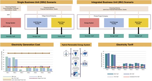
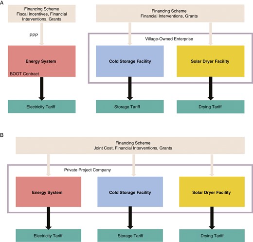
To assess the feasibility of the project, two scenarios of the business model were assessed using the cash flow method (Fig. 4). The first was the single-business unit (SBU) scenario, in which the HRES and the productive sector were two separate business units. Specifically, the HRES was financed through public–private partnership under a build–own–operate–transfer contract and the productive sector project used the village-owned enterprise (Badan Usaha Milik Desa, BUMDes) business model. The user would pay a processing fee to productive facilities based on the processing load per usage. The CAPEX for the productive facilities was derived from the market price of existing equipment and the OPEX comprised the cost of materials, labour, and maintenance and utilities, as well as the expenditure on taxes, insurance and depreciation. The internal rate of return (IRR) was set at a fixed rate of the weighted average cost of capital (WACC) + 2% to determine the tariff for each system.
Business model for (a) the SBU and (b) the IBU scenarios
In the integrated business unit (IBU) scenario, the productive sectors were integrated with the HRES under a joint business. The power plant was managed by a private project company with a power purchase agreement (PPA) with PLN. The private entity also managed productive activities business. A joint cost system applied to the electricity generation costs that were charged to the power generation business unit and the productive activity business unit. The split point was when electricity would be distributed. Therefore, the investment in productive activities would be higher because the investment in power generation would be lower. The productive facilities did not have electricity costs because electricity was used for the generation cost.
Financing schemes were developed for each business model, considering current regulations and fiscal incentives. Tables 2 and 3 present the financing schemes proposed for the energy system and the productive sectors, respectively. The proposed financial incentives are partial grants (FSE-4, FSE-5, FSE-6) and a full grant (FSE-3) to waive capital expenditures. Proposed fiscal incentives are a lower tax rate and tax allowances (FSE-2, FSE-5, FSE-6) based on Government Regulation (PP) No.78/2019 [73] and PPh Act No. 31E(1) [74]. We also propose a soft loan at a low debt rate of 1.02% [75] over a 19-year loan term (FSE-5, FSE-6). Financing schemes for productive sectors include government grants for main process equipment procurement [76, 77] (FSP-3, FSP-5) and a soft loan with a 6% debt rate over a 7-year loan term [78] (FSP-4, FSP-5).
Financing schemes for the SBU (energy system) and IBU (energy system and productive sectors) scenarios
| Financing schemes | Description | % Equity | % Debt; cost of debt | Grant | Income tax |
|---|---|---|---|---|---|
| FSE-1 | Business as usual | 20% | 80%; 4.13% | – | 22% |
| FSE-2 | Fiscal incentive relative to FSE-1 | 20% | 80%; 4.13% | – | 11% + tax allowance |
| FSE-3 | Financial intervention | – | – | 100% | 22% |
| FSE-4 | Financial intervention relative to FSE-1 | 20% | 80%; 4.13% | 75% | 22% |
| FSE-5 | Soft loan, financial intervention, fiscal incentive | 20% | 80%; 1.02% | 65% | 11% + tax allowance |
| FSE-6 | Financial intervention relative to FSE-5 | 20% | 80%; 1.02% | 75% | 11% + tax allowance |
Financing schemes for productive sectors in the SBU scenario
| Financing schemes | Description | % Equity | % Debt; cost of debt | Grant | Income tax |
|---|---|---|---|---|---|
| FSP-1 | Investor funding | 100% | – | – | 22% |
| FSP-2 | Business as usual | 40% | 60%; 8.67% | – | 22% |
| FSP-3 | Financial intervention relative to FSP-2 | 40% | 60%; 8.67% | Yes | 22% |
| FSP-4 | Soft loan relative to FSP-2 | 40% | 60%; 6% | – | 22% |
| FSP-5 | Soft loan relative to FSP-3 | 40% | 60%; 6% | Yes | 22% |
1.5.2 Job creation
We performed a job creation analysis as an impact of HRES development by calculating the job factor of each system component as direct employment in jobs–year/MW and as indirect employment in jobs/MW, where MW is the peak energy production of the component [79]. This study used the following job factor values: 30 jobs/MW for the solar PV panel [80], 22 jobs/MW for the WT [80] and 0.01 jobs/MWh for the battery [79].
The calculation can be done using Equation (7) as suggested by Sawle et al. [79]:
where JCPV, JCWT and JCBAT are the job factor for the solar PV panel, the WT and the battery, respectively; PPV is the solar PV panel peak power generation (MWp); PWT is the power generated from the WT (MW); and EBAT is the nominal battery capacity (MWh).
Additional employment due to the development of productive activities was calculated using Equation (8), based on Peters et al. [81]:
where OL is the operating labour required, n is the number of process steps, fOL is the operating labour factor in employee–hours/day–processing step and tops,ann is annual operating days.
2 Results and discussion
2.1 Electricity demand
Mahaleta’s energy demand was classified into the following three sectors based on load usage patterns: residential, community and commercial, and productive. The load profile was differentiated for weekdays and weekends due to different usage patterns in the community and commercial sectors. The total estimated demand load was 705.3 kWh/day on weekdays and 674.2 kWh/day on weekends. Fig. 5 visualizes the hourly load profile for weekdays and weekends.
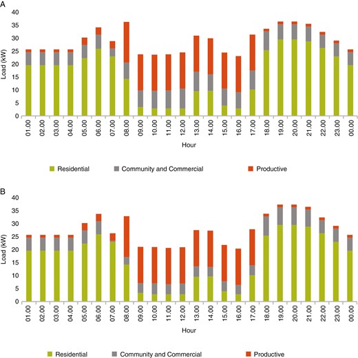
Hourly load profile for (a) weekdays and (b) weekends
The electricity demand in the residential sector was assumed to be the same throughout the year, since the village is located in a tropical country where the climate tends to be uniform all year round; therefore, the electricity load does not experience significant changes [52]. There is also no difference in the consumption pattern on weekdays versus weekends because villagers tend to follow the same routines consistently compared with the varying routines of urbanites. The estimated load for the residential sector is 398.04 kWh/day, which is an average of 4.15 kWh/day per household. Compared with the standard household electricity consumption of the Ministry of Energy and Mineral Resources (MEMR) of 6 kWh/day [82], the estimated load is relatively lower because people in remote areas use simpler appliances with different usage patterns. The electricity consumption of the residential sector is mainly to power lighting, televisions, refrigerators and fans. The load increases in the morning (05:00–06:00) as people prepare for the day. The peak load occurs at night (19:00–20:00) due to high activity in the home as people prepare to rest. The residential load is low during the day because most people are involved in activities outside the house.
The load for the community and commercial sector was estimated at 143.74 kWh/day for weekdays and 112.65 kWh/day for weekends. On weekdays, electricity demand is high at facilities such as schools, the public health centre and the village office during working hours (08:00–17:00), whereas on weekends, the demand is lower because these facilities are closed; on weekends, the demand comes mainly from church activities, shops and restaurants.
The productive load was estimated at 163.52 kWh/day and was dominated by drying activities. Productive sector activities were assumed to occur daily, resulting in no load difference between weekdays and weekends. The peak load occurs in the morning because drying, freezing and cooling activities occur simultaneously. The electricity demand for cold storage is lower than that for drying because, with cold storage, only the freezing process is high energy, whereas less energy is required to maintain the cold temperature because the flow of heat from the environment into the system can be minimized by reducing the frequency of opening and closing the cold room [83]. The energy requirement for the drying system is higher because fans and blowers must work continuously with a constant load throughout the drying process.
2.2 HRES
HOMER optimized all the possible system configurations under given inputs that satisfy all the predefined constraints [58]. Table 4 presents optimization results for three possible system configurations of solar PV, WT and battery.
Optimization results
| Configuration | PV (kW) | Wind turbine (number) | Battery (number) | Converter (kW) | Capital cost ($) | O&M cost ($/year) | NPC ($) | COE ($/kWh) | Capacity shortage (%) |
|---|---|---|---|---|---|---|---|---|---|
| PV/WT/BAT | 271.62 | 1 | 132 | 78.31 | 683 335 | 19 990 | 920 636 | 0.305 | 0 |
| PV/BAT | 482.84 | – | 165 | 81.47 | 752 539 | 20 176 | 992 048 | 0.329 | 0 |
| WT/BAT | – | 2 | 9042 | 52.5 | 11 035 679 | 719 880 | 19 581 230 | 6.490 | 0.1 |
BAT, battery.
The HRES depicted in Fig. 6 as comprising solar PV panels, a WT and a battery is the optimal system based on the lowest cost optimization. Fig. 7 shows the monthly electricity production. The optimal system produces 667 041 kWh/year of total electrical energy, of which solar PV panels produce 499 037 kWh/year (74.8%), and the WT produces the remaining 168 004 kWh/year (25.2%). The capacity factors of the PV array and WT are 21% and 24%, respectively. The large installed capacity of PV is to ensure that there is always enough energy available to meet the demand for electricity due to the intermittent nature of variable RE where electricity is generated when the resource is available, rather than when it is required, causing a mismatch in energy supply and demand [84–86]; the amount of energy supply is highest during the day, while the peak demand for electricity occurs at night. Thus, the excess production generated by the PV system is used to charge the batteries that will be used to supply electricity at night. It is also because the production of the WT itself is insufficient to meet the electricity demand or to charge the battery.

Hybrid renewable energy system configuration. Image from HOMER Pro modelling software used with permission from UL Solutions.
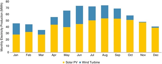
Monthly electricity production
The optimal system configuration can meet all electrical loads (i.e. unmet load = 0 kWh/year). Generally, the HRES always produces surplus electricity. Wagner [87] found that surplus electricity is no less than 25% of total electricity produced from intermittent sources. According to Li et al. [88], the production surplus from a PV–wind system ranges from 57% to 70%. The surplus of the system designed in this study is 57.9%.
Fig. 8 shows the system dispatch. The dispatch strategy for the selected battery is load following, where the battery is charged only when there is surplus electricity production, so there are no costs associated with charging the battery [58]. On the day shown, PV array electricity production occurred from 06:00 to 18:00, with the most production occurring at 12:00. The WT produced a minimal amount of electrical energy throughout the day, as indicated by the low line. From 07:00 to 17:00, there was excess electricity production, so the battery was charging during that period. The electrical input to the battery decreases from 10:00 onwards due to the lower maximum energy that can be stored by the battery as it approaches the full state of charge. At night, when there is no solar irradiation and the WT output is low, the battery discharges from 17:00 to 07:00 the next day to meet the peak load that occurs at night. Excess electricity that is not used to meet electricity demand and charge batteries can be used to contribute to meeting increased electricity demand in the future and support the improvement of the socio-economic conditions of the rural community; it can also can be distributed to electrify other nearby villages.
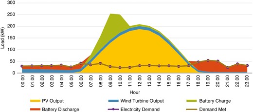
System dispatch
The proposed HRES is entirely renewable but, considering the life-cycle emissions of each component, system operation would result in emissions of 26.8 tons CO2-eq/year. For comparison, if the same electricity demand were to be fulfilled entirely by a diesel power plant, as is common practice in electrifying remote regions of Indonesia, the amount of CO2 emissions from the diesel power plant would be 312 tons CO2-eq/year. Therefore, developing a HRES would significantly reduce CO2 emitted into the environment by 91%, as shown in Fig. 9.
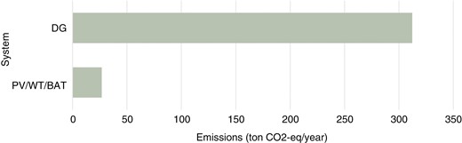
CO2 emissions associated with the system configurations
2.3 Electricity production costs and tariffs
2.3.1 Productive sectors
Our design of the cold-storage system has a capital cost of $29 593 and an annual operating cost of $25 554. Cold-storage machines and supporting equipment account for the largest share of the capital cost of the cold-storage system due to the large storage capacity needed, while workers’ salaries account for the largest share of the operating cost. The price of the fish to be stored in cold storage was not included in the operating cost because fishermen pay the storage fee based on the weight of the fish and the storage duration. Table 5 shows the feasibility of each cold-storage facility financing scheme.
Feasibility of cold-storage financing schemes
| Financing schemes | NPV ($) | IRR (%) | PBP (years) | Storage cost ($/kg) | Tariff ($/kg) | Feasibility |
|---|---|---|---|---|---|---|
| FSP-1 | 4194.92 | 14.38 | 7 | 0.037 53 | 0.038 31 | Feasible |
| FSP-2 | 5126.70 | 13.26 | 7 | 0.037 25 | 0.038 12 | Feasible |
| FSP-3 | 3723.72 | 13.26 | 7 | 0.034 81 | 0.035 44 | Feasible |
| FSP-4 | 5805.31 | 12.01 | 8 | 0.036 58 | 0.037 44 | Feasible |
| FSP-5 | 4227.65 | 12.01 | 8 | 0.034 33 | 0.034 96 | Feasible |
PBP, payback period.
Storage costs for all schemes were considered economically feasible, with FSP-5 having the lowest cold-storage system tariff and receiving a grant in the form of cold-storage equipment, as well as soft loans for funding. Fig. 10 compares the tariff of the facility with the MMAF freezing and storage tariff of $0.0359/kg [89]. The comparison shows that the FSP-3 and FSP-5 tariffs are below the MMAF rate because of the waived capital cost from the grant.
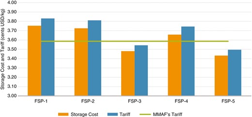
Cold-storage cost and tariff
Although the scale is smaller than the integrated cold storage of the MMAF, the low tariff is possible because the cold-storage system designed in this study is portable and has fewer processing units, and the processing is performed manually, whereas, with integrated cold storage, where the processing unit is more complex and the processing uses more machines [90], the capital cost and operating costs are higher.
The solar dryer facility has a capital cost of $376 297 and an annual operating cost of $49 892. Solar dryer equipment accounts for the largest portion of the capital cost due to the large capacity and high energy requirements of drying. The operating cost mainly comprises maintenance costs as a result of the large number of solar collectors. The price of wet seaweed was not included in the operating costs because farmers pay the drying fee based on the weight of the wet seaweed.
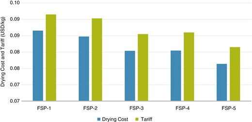
Table 6 shows the feasibility of each solar drying facility financing scheme. The drying costs for all schemes were considered economically feasible, with FSP-5 having the lowest drying tariff, as shown in Fig. 11, given the receipt of a grant in the form of the main solar drying equipment as well as soft loans for funding. Compared with drying tariffs in Indonesia, which range from $0.07/kg to $0.18/kg [91, 92], as well as those in East Africa and India, which are $0.07/kg [93] and $0.058/kg [94], respectively, the tariffs in all proposed schemes are in a competitive range.
Feasibility of seaweed drying financing schemes
| Financing schemes | NPV ($) | IRR (%) | PBP (years) | Drying cost ($/kg) | Tariff ($/kg) | Feasibility |
|---|---|---|---|---|---|---|
| FSP-1 | 52 929.83 | 14.38 | 7 | 0.087 | 0.092 | Feasible |
| FSP-2 | 64 668.65 | 13.26 | 7 | 0.085 | 0.090 | Feasible |
| FSP-3 | 59 693.52 | 13.26 | 7 | 0.080 | 0.086 | Feasible |
| FSP-4 | 73 149.83 | 12.01 | 8 | 0.080 | 0.086 | Feasible |
| FSP-5 | 67 549.19 | 12.01 | 8 | 0.076 | 0.082 | Feasible |
Cost and tariff of seaweed drying
2.3.2 Electricity system
According to the results of the HRES simulation, the optimal solution results in an NPC of $920 636 and a LCOE of $0.305/kWh. The system costs are listed in Table 7. The capital cost is dominated by solar PV modules, which account for a 40% share due to the large number of modules needed. Regarding the replacement costs, battery replacement accounts for 70% due to the short life of the battery. WTs account for 50% of the share of O&M costs for periodic repairs and the replacement of spare parts.
Energy system costs
| Cost component | Amount ($) |
|---|---|
| Capital cost | 683 335.24 |
| Replacement cost | 161 593.23 |
| O&M cost | 107 283.39 |
| Salvage value | –31 575.48 |
| Total | 920 636.38 |
| Cost component | Amount ($) |
|---|---|
| Capital cost | 683 335.24 |
| Replacement cost | 161 593.23 |
| O&M cost | 107 283.39 |
| Salvage value | –31 575.48 |
| Total | 920 636.38 |
The positive cash flow for the HRES comes from the electricity sales of the project company to PLN at the electricity purchase price set for RE power plants, which is 85% of the electricity production cost [95]. Electricity production cost refers to the sum of capital costs with O&M, fuel and environment costs. Since the system is located in an off-grid area, the production cost used was that for small subsystems in the Maluku and Papua regions, which is 2805 IDR/kWh or $0.1935/kWh [96]. Therefore, the electricity purchase price charged to PLN was $0.1645/kWh, assuming that PLN purchases all the electricity produced.
Tables 8 and 9 show the feasibility of each financing scheme in the SBU and IBU scenarios, respectively. In the SBU scenario, the only feasible scheme is FSE-3, in which financing comes entirely from grants that waive the capital cost. For FSE-1 and FSE-2, the negative value in the payback period means that the project is not feasible under these financing schemes because the payback period would not be completed at the end of the project lifetime. In the IBU scenario, although the payback period for feasible scenarios is lengthy, it is always shorter than the project lifetime, rendering those scenarios still feasible. To make the investment profitable, the percentage of grant funds required must be >75%. The current funding ratio and fiscal incentive policies do not have a significant effect on reducing the COE from RE sources.
Feasibility of SBU scenario electricity system financing schemes
| Financing schemes | NPV ($) | IRR (%) | PBP (years) | Production cost ($/kWh) | Feasibility |
|---|---|---|---|---|---|
| FSE-1 | –1 161 373 | –11.52 | –18 | 0.6228 | Not feasible |
| FSE-2 | –1 154 340 | –10.37 | –18 | 0.5926 | Not feasible |
| FSE-3 | 209 499 | – | 0.5 | 0.0808 | Feasible |
| FSE-4 | –119 672 | –0.05 | 14 | 0.2105 | Not feasible |
| FSE-5 | –200 068 | –2.41 | 1 | 0.2391 | Not feasible |
| FSE-6 | –76 842 | 1.51 | 14 | 0.1930 | Not feasible |
Feasibility of IBU scenario electricity system financing schemes
| Financing schemes | NPV ($) | IRR (%) | PBP (years) | Production cost ($/kWh) | Feasibility |
|---|---|---|---|---|---|
| FSE-1 | –826 696 | –0.11 | 13 | 0.5689 | Not feasible |
| FSE-2 | –763 277 | 0.71 | 12 | 0.5137 | Not feasible |
| FSE-3 | 203 568 | 9.97 | 11 | 0.0215 | Feasible |
| FSE-4 | –42 642 | 6.26 | 12 | 0.1576 | Not feasible |
| FSE-5 | –52 732 | 6.18 | 12 | 0.1599 | Not feasible |
| FSE-6 | 42 268 | 7.33 | 11 | 0.1141 | Feasible |
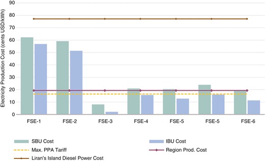
Fig. 12 compares the electricity production cost and the system tariff with the PLN tariff. The tariff that PLN charges customers [97] is lower than the tariff for all schemes except FSE-3. Compared with the PLN subsidized electricity tariff, which reflects the purchasing power of customers in the outermost island villages, ranging from 800 to 1000 IDR/kWh or $0.055–0.065/kWh [98], the entire tariff on the proposed financing schemes is above the purchasing power of the residents.
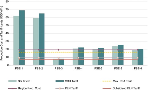
Electricity cost and tariff for the SBU scenario
In Indonesia, the electricity tariff is uniform in all regions due to the structure of the country’s electricity market, which is a single-buyer industry by a state-owned electricity company. The tariff only differs according to consumer categories, which are household, commercial and industrial. However, the LCOE might be different depending on the system configuration and capacity. The comparison of LCOE with other locations in Indonesia with similar location remoteness is shown in Table 10. Diesel generators are still widely used for power generation in remote locations and currently are still heavily subsidized by the government. However, as PLN increases its efforts to decarbonize the power system, diesel power plants are now beginning to be hybridized with renewable sources such as PV and wind, until a more cost-effective power generation option is viable [99].
LCOE comparison with other locations
| No. | Location | System | Capacity | LCOE ($/kWh) | Reference |
|---|---|---|---|---|---|
| 1 | Temajuk Village, West Kalimantan | PV/WT/BAT | 2 kW | 0.751 | [62] |
| 2 | Koak Village, East Nusa Tenggara | PV/WT/BAT | 8.11 kW | 0.463 | [100] |
| 3 | Seram Island, Maluku | PV/WT/DG | 20 MW | 0.204 | [101] |
| 4 | Eastern Indonesia | DG/PV/WT/BAT | 50.8 MW | 0.155 | [102] |
| 5 | Villages in Sulawesi and Sumatera regions | PV/BAT | 232.5 kW | 0.580 | [6] |
| 6 | Sabu Island, East Nusa Tenggara | PV/BAT | 1 MW | 0.305 | [103] |
| 7 | Teupah Island, Aceh | PV/DG/BAT | 444 kW | 0.246 | [104] |
| 8 | Karimun Jawa Island | PV/DG | 4.59 MW | 0.260 | [105] |
| 9 | A village in East Nusa Tenggara | PV/DG | 200 kW | 0.570 | [106] |
| 10 | Mahaleta, Southwest Maluku | PV/WT/BAT | 351.62 kW | 0.305 | This study |
BAT, battery.
LCOE varies depending on the system configuration and capacity, as well as location. The LCOE of this study is still within the range of other hybrid systems in remote locations. Systems with the same PV/WT/BAT configuration but different size (1, 2, 10) result in higher LCOE for the system with smaller capacity. Systems with roughly the same size but with different configurations (5, 7, 9, 10) show that the LCOE of fully renewable systems is slightly higher than those of hybrid systems with diesel generators aside due to smaller power plant capacity, also because variable RE sources generally have lower capacity factors than diesel generators. Large systems with different configurations (3, 4, 6, 8) that are hybridized with more RE tend to have lower LCOE since the systems can produce more electricity and are less dependent on diesel generators. On the basis of the above comparison, the COE production in this study is still within the range of other remote locations.
The regulation of the maximum price of the PPA, which is only 85% of the regional production cost [95], greatly affects the feasibility of the proposed schemes. If the regulation sets a 100% electricity purchase price from the production cost, the economic feasibility of FSE-4 and FSE-6 will increase. The effect of this PPA price is attributable to the fact that the existing production cost is a production cost for generation using not RE generators, but rather diesel power plants. The cost of generating RE is still higher because, despite relatively low O&M costs, the capital cost to build RE plants remains high. Therefore, incentives to reduce initial investment costs, such as grants, are needed to increase the bankability of RE projects [107]. In addition to incentives, financial and business innovations achieved by combining commercial and government funding and implementing supportive policies can reduce the cost and risk associated with RE projects [108].
The usage fees for the drying and cold-storage systems were set, based on the literature, at $0.058/kg [94] and $0.101/kg/day, respectively [46]. Tariff setting was adjusted to reflect the same technology and scale.
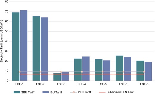
In the IBU scenario, FSE-3 and FSE-6 were considered economically feasible as evidenced by the production cost being below the maximum price of the PPA and the positive net present value. Economically viable financing schemes include financial assistance in the form of grants and fiscal incentives. Fig. 13 compares the system production cost and electricity tariffs with the PLN production cost and tariff.
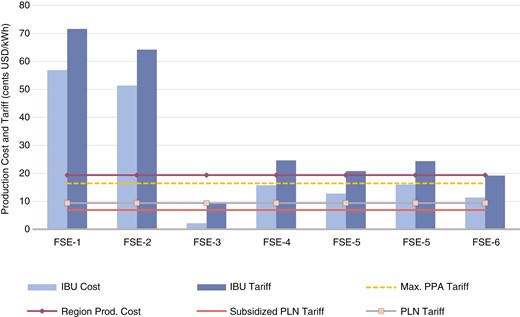
Electricity cost and tariff for the IBU scenario
Fig. 14 compares the electricity production costs in the two scenarios. The cost in the IBU scenario is 5.3–10.4% lower than the cost in the SBU scenario due to the joint cost system applied in the former scenario, which yields lower capital costs and operating costs for the energy system. Additionally, the utilization rate showed an increase because electricity would be used for productive and domestic activities. The operation of productive activities increases the income of the rural community, which increases the purchasing power of the community, thus increasing the investment viability of the renewable power project.
Comparison of electricity production costs
Some financing schemes exceed the regional production cost or the small subsystem cost set by the MEMR [96]. However, in reality, in the outermost islands, the production cost is generally much higher due to accessibility constraints and environmental factors when distributing electricity. For example, the cost for a 300-kW diesel generator power plant on nearby Liran Island, Southwest Maluku, is 11 182 IDR/kWh or $0.771/kWh [109]. Thus, compared with this case, all financing schemes would result in lower generation costs.
Fig. 15 compares the tariffs in the two scenarios. The tariffs in the IBU scenario are lower, except for FSE-1, FSE-3 and FSE-4, which have higher tariffs compared with the SBU scenario. This is because the financing scheme does not include fiscal incentives. Thus, it can be concluded that fiscal incentives allow independent power producers to sell electricity at a lower rate due to the tax allowance. All financing schemes except for FSE-3 have a production cost that is much higher than the people’s purchasing power.
Electricity tariff comparison
Electrifying 3T regions requires government intervention, not only from the supply side for RE power generation activities, but also from the demand side, which refers to the economic capability of the community. This intervention can be in the form of subsidizing electricity tariffs so that electricity is affordable to people with low purchasing power who live in 3T regions.
The use of the RE power system can contribute to reducing the government subsidy to ensure the affordability of electricity for residents of 3T regions. The proposed PV/WT/battery system can reduce the subsidy by $0.1484/kWh or 21.13% (Fig. 16) compared with the amount of subsidy given for electricity generated by the diesel power plant currently operating in the region. The annual subsidy savings would be $98 968, which can be allocated to subsidize the capital required to develop the HRES, thus improving the viability of the system.
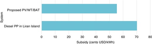
Subsidy comparison of the diesel power plant and the PV/WT/battery power plant
2.4 Socio-economic effects
2.4.1 Job creation
Developing an HRES and productive activities in Mahaleta would create additional job opportunities for the local community. The solar drying facility would require a staff of three and the cold-storage facility would add two jobs. The HRES would create 12 additional employment opportunities, namely 9 jobs related to solar PV panels, 2 related to the WT and 1 related to the battery. Therefore, a total of 17 jobs would be created in a village community where 132 residents are in the productive age range. Thus, an HRES and productive activities would create employment for 13% of the productive age population.
2.4.2 Product economic benefits
Drying seaweed using a solar dryer, which is done in a closed space, can improve the quality of the seaweed, which in turn would increase the sale value of the dried seaweed. The market price for wet seaweed is $0.344/kg [110], while seaweed dried using the conventional method is sold at $1.03/kg. However, the retail value for dry seaweed can be as much as $2.07/kg [111]. Compared with conventional drying in an open space, using a solar dryer could minimize exposure to environmental contamination. Additionally, the use of a solar dryer could ensure optimal seaweed drying during the rainy season because the drying is carried out under controlled operating conditions. Therefore, improving product quality through solar drying could increase the income of the local community’s seaweed cultivation by 50%—that is, from $205 337/year to $410 713/year.
Furthermore, with adequate electricity facilities, locals could utilize cold storage to prolong the shelf life of their fishery produce. If the freshness of the fish can be preserved, the commodity can be distributed to a wider market. In addition, cold storage is a tool for avoiding higher prices due to food scarcity during famine in conditions under which fishermen cannot fish in the sea. Fish can be stored in cold storage to ensure guaranteed availability of food stocks, allowing the stabilization of fish prices.
3 Conclusions
This study evaluated the design of an HRES comprising solar PV panels, a WT and batteries for powering the residential, community, commercial and productive sectors in Mahaleta in eastern Indonesia. The selected case study represents the prospective implementation of an HRES in underdeveloped rural regions considering productive sectors, with electrification potentially improving the welfare of residents. Optimization based on the lowest cost objective function resulted in the most optimum configuration of 271.62 kW of solar power, 80 kW of wind power and 132 batteries with a NPC of $920 636 and COE production of $0.305/kWh. The configuration has 0% capacity shortage and 0 kWh/year unmet load, meaning that it can always fulfil the village electricity demand. Additionally, it was found that the implementation of an HRES can significantly reduce CO2 emissions by 91% compared with the use of a diesel generator.
Developing an HRES as a separate business entity is only economically viable with full-grant financing and an electricity tariff of $0.08/kWh. However, when integrated with productive activities, the HRES would be viable with 75% grant funding, soft loan financing and fiscal interventions in the form of tax allowances and lower taxes.
In this study, all financing schemes for the productive sector were deemed economically feasible. The lowest tariffs were $0.0349/kg for cold storage and $0.0815/kg for seaweed drying, with the development of facilities financed through grants and soft loans. It was also found that integrating an HRES with productive activities can create employment opportunities for 13% of the productive age population in the village and boost local income by increasing the value of dried seaweed sales.
A more rigorous government intervention in electricity provision to remote rural villages and underdeveloped regions is recommended to attract private-sector participation. Developing an RE system is a key driver for economic development in local communities, but the impact of energy access would go beyond the financial aspect to improve welfare and national security.
Nomenclature
| Total annualized cost of the system ($/year) | |
| Cost associated with component i over the planning horizon ($) | |
| Total net present cost ($) | |
| Deferrable electrical load served (kWh/year) | |
| Total electrical demand (kWh/year) | |
| Electricity generation (kWh/year) | |
| Non-renewable electrical production (kWh/year) | |
| Primary electrical load served (kWh/year) | |
| Total electrical load served (kWh/year) | |
| Capacity shortage fraction | |
| Renewable fraction | |
| Non-renewable thermal production (kWh/year) | |
| Total thermal load served (kWh/year) | |
| Maximum annual capacity shortage (%) | |
| Initial investment ($) | |
| Net cash flow from each component ($) | |
| Operating reserve as a percentage of load in the current time step (%) | |
| Load in time step t (kWh) | |
| Salvage value of component i ($) | |
| Planning horizon (years) | |
| Time of the cash flow (years) | |
| Discount rate (%) |
Acknowledgements
The authors are grateful to the Faculty of Engineering Universitas Indonesia for supporting this work financially under the Seed Grant Professor FTUI, Contract Number: NKB-1966/UN2.F4.D/PPM.00.00/2022.
Conflict of interest statement
None declared.
Data Availability
Public sharing for data underlying this article is not applicable because the data are owned by the government and company, and were obtained by the authors through permission.
