


Abstract
The Brazilian Atlantic Forest (BAF) is one of the most impacted biomes in the world, and in this region, there are several examples of the effects of Pleistocene climate changes among the species found there. Athenaea fasciculata (Solanaceae) is a forest component distributed mainly throughout the BAF extension. Here, we investigated the genetic diversity and population structure of A. fasciculata based on plastid and nuclear markers, aiming to better understand the impact of Pleistocene climate changes on BAF vegetation. We used population genetics, demographic methods and ecological niche modelling coupled to an evolutionary approach to describe the species distribution across time. The phylogeographic analysis of A. fasciculata indicated that Pleistocene climate changes played an important role in its evolution. The species is structured in two groups of populations that emerged from different refugia and were under different climate influences, supporting previously proposed connections between the Atlantic and Amazon Forests, the two most important Neotropical rainforests.
INTRODUCTION
The Brazilian Atlantic Forest (BAF) is one of the most diverse and endangered biomes in the world; it displays a high abundance of endemic species and is under intense anthropogenic pressures (Myers et al., 2000; Haddad et al., 2015). At present, only c. 10–30% of the original coverage remains (Rezende et al., 2018) in a highly fragmented landscape (Supporting Information, Fig. S1), which increases edge effects and low connectivity among fragments (Tabarelli, Silva & Gascon, 2004; Ribeiro et al., 2009; Haddad et al., 2015).
The BAF occupies an area of complex topography, which originated due to climatic and sea-level changes during the Pleistocene (Suguio et al., 2005), and it shows strong seasonality, sharp environmental gradients and orographic-driven rainfalls as a consequence of winds from the tropical Atlantic Ocean. All these characteristics influenced the formation of landscapes that intersperse patches of forest with grasslands (Behling & Lichte, 1997; Behling, 1999, 2002; Behling & Negrelle, 2001).
Efforts have been made to understand the factors that led to biological diversification in the BAF and to reconstruct its evolutionary history. Several studies proposed that this forest experienced expansions (Auler et al., 2004) and contractions (Carnaval & Moritz, 2008; Carnaval et al., 2009) in response to climatic changes during the Quaternary period (Leite et al., 2016). Phylogeographic evidence has also suggested past fragmentation (Pellegrino et al., 2005; Lacerda, Marini & Santos, 2007; Thomé et al., 2010; Ribeiro et al., 2011) that may be explained by forest refuge theory (Haffer, 1969). Indeed, two main refugia (Carnaval & Moritz, 2008) were identified in the BAF: a large central Late Quaternary refuge (from Rio de Janeiro to Bahia) and a small northern refuge (in Pernambuco and Alagoas), both corroborated by additional phylogeographical studies of several animal and plant species (Carnaval et al., 2014). Other minor refugia, such as the São Paulo refuge (Carnaval et al., 2009) and Subtropical Highland Grasslands (SHG) (Barros et al., 2015) have been found for some species.
The forest refuge model has been extensively tested, but despite its broad acceptance, some species do not fit this model and display more complex evolutionary scenarios (Turchetto-Zolet et al., 2013; Leal, Palma-Silva & Pinheiro, 2016). The putative interplay between sea-level changes and land distribution in the Brazilian continental shelf was presented as a main alternative hypothesis to explain the BAF dynamics over time. This hypothesis explains why, for some species of forest-specialist small mammals, populations expanded during the last glacial period, which is not expected according to the forest refuge theory (Leite et al., 2016).
Athenaea fasciculata (Vell.) I.M.C.Rodrigues & Stehmann (Solanaceae) is a shrub or small tree that occurs mainly throughout the BAF, with some documented occurrence in the Paraná Basin (Fig. 1, Supporting Information, Fig. S1) and is a member of Withaniinae (Olmstead et al., 2008). Although it has diverse habitat preferences and several known populations (Caiafa & Martins, 2010), it is considered a rare species with a small number of individuals per population (Table 1) and, unlike other plant species, it is found at diverse elevations. Initially described as Aureliana fasciculata (Vell.) Sendtn. (in Martius, Fl. Bras. 10: 140. 1846) this species was considered restricted to the BAF. With the most recent nomenclatural revision (Rodrigues, Knapp & Stehmann, 2019), this taxon is now named Athenaea fasciculata and, including all synonyms, it is recorded from northern and north-eastern Brazil to north-eastern Argentina, Paraguay, Bolivia and Peru.
Sampling information for A. fasciculata
| Code | Groupa | Location | N | Geographical coordinates | Elevation (m a.s.l.) | Voucherb |
|---|---|---|---|---|---|---|
| Afasc1 | A | Road BA-270/Itacaré, BA# | 5 | 15 25’ 14”S, 39 16’ 13”W | 497 | BHCB126144 |
| Afasc2 | A | Conservation Area Serra Bonita, Camacan, BA | 15 | 15 23’ 10”S, 39 34’ 04”W | 662 | BHCB126175 |
| Afasc3 | A | Talismã, Santa Maria do Salto, MG | 1 | 16 24’ 34”S, 40 02’ 45”W | 843 | BHCB126176 |
| Afasc4 | A | Itaúnas, ES | 4 | 18 25’ 08”S, 39 42’ 29”W | 7 | SAMES 5532 |
| Afasc5 | A | Teresópolis, RJ | 7 | 22 24’ 33”S, 42 45’ 19”W | 379 | BHCB145091 |
| Afasc6 | A | Itatiaia National Park, RJ | 12 | 22 26’ 52’’S, 44 36’ 09”W | 934 | BHCB145033 |
| Afasc7 | A | Trindade, RJ | 4 | 23 20’ 48’’S, 44 43’ 18”W | 65 | BHCB115994 |
| Afasc8 | B | João Monlevade, MG | 2 | 19 49’ 28’’S, 43 10’ 42”W | 834 | NA |
| Afasc9 | B | Itatiaia National Park, Itamonte, MG | 4 | 22 22’ 19’’S, 44 44’ 53”W | 1957 | BHCB145057 |
| Afasc10 | B | Road Paraty-Cunha, Cunha, RJ | 9 | 23 11’ 39’’S, 44 49’ 44’’W | 1019 | BHCB115989 |
| Afasc11 | B | Conservation Area Japi, Jundiaí, SP | 16 | 23 14’ 53’’S, 46 56 20’’W | 1137 | BHCB115929 |
| Afasc12 | B | Road SP-088, Biritiba Mirim, Salesópolis, SP | 4 | 23 33’ 51’’S, 46 00 54’’W | 780 | BHCB115976 |
| Afasc13 | B | Paranapiacaba, Santo André, SP | 14 | 23 47’ 13’’S, 46 18’ 18”W | 813 | BHCB 145011 |
| Afasc14 | B | Quatro Barras, PR | 13 | 25 22’ 47”S, 49 02’ 16”W | 911 | MBM 76042 |
| Afasc15 | B | Bituruna, PR | 6 | 26 04’ 30”S, 51 40’ 49”W | 951 | BHCB 143441 |
| Afasc16 | B | Itaiópolis, SC | 8 | 26 32’ 58”S, 49 46’ 30”W | 933 | BHCB 143439 |
| Afasc17 | B | Department Guarani, Province Missiones (Argentina) | 2 | 26 52’ 23”S, 54 13’ 50”W | 483 | NA |
NA—not available; a Group A or B based on results; # Brazilian states abbreviations: BA, Bahia; ES, Espírito Santo; MG, Minas Gerais; PR, Paraná; RJ, Rio de Janeiro; SC, Santa Catarina; and SP, São Paulo; m a.s.l. - meters above the sea level; bBHCB: ‘Universidade Federal de Minas Gerais’ Herbarium; MBM—Herbário do Museu Botânico Municipal; SAMES—herbário São Mateus, ES.
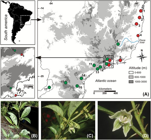
A, Geographical location of collection sites (populations) of individuals of Athenaea fasciculata collected across Atlantic Forest (Brazil). Red dots correspond to the genetic group A and green dots to the B. B, General view of adult plant branch. C, Athenaea fasciculata immature fruits highlighting the calyx. (D, Flower morphology.
Here, genetic variability and demographic history of A. fasciculata were assessed based on two segments of the plastid genome and one nuclear region. We investigated how the genetic diversity and structure of A. fasciculata might reflect different scenarios already observed for BAF species: (1) phylogeographic discontinuities could be attributed to rivers acting as barriers, such as the Doce River as described for a species of Passiflora L. with a similar distribution (Cazé et al., 2016); (2) despite the species being forest specialist, its origin was older than Pleistocene and genetic diversity and structure were not influenced by forest expansion and retraction, as was described to small mammals from the BAF (Leite et al., 2016); (3) higher genetic diversity should be observed in populations found in previously proposed refuge areas, such as the Late Quaternary refuge as observed in some species (Carnaval & Moritz, 2008; Barros et al., 2015) and (4) A. fasciculata populations could be structured according to ecological differences observed along with the BAF, highlighting the importance of regions of habitat stability (D’Horta et al., 2011).
MATERIAL AND METHODS
Plant material
Athenaea fasciculata is a shrub or small tree, usually with white-greenish flowers displaying green, brown or purple maculae (Fig. 1), which inhabit sub-forests or glades from the sea level to c. 2000 m in elevation (Hunziker, 2001). Based on morphological traits, the species is considered to be bee-pollinated (Cocucci, 1999), and fruits and seeds could be mammal-dispersed (Martins, Cazotto & Santos, 2014). We collected 126 individuals of A. fasciculata from 17 sites (hereafter called populations; Table 1) throughout the species range in the BAF (Fig. 1). Fresh leaf tissues were sampled from each individual and preserved in silica gel. For voucher information, see Table 1.
Dna extraction, amplification and sequencing
Genomic DNA was extracted from young dry leaves with the Nucleo Spin Plant II kit (Macherey-Nagel, Düren, Germany) using the manufacturer’s protocol. Two plastid intergenic regions, trnH-psbA (Sang, Crawford & Stuessy, 1997) and trnS-trnG (Hamilton, 1999), and the nuclear ribosomal internal transcribed spacers (ITS) (Desfeux & Lejeune, 1996) were amplified through PCR with previously described protocols (Lorenz-Lemke et al., 2006 for plastid regions; Zamberlan et al., 2015 for ITS). We used 30–50 ng of template DNA in each PCR, which was purified using polyethylene glycol precipitation (PEG 20%) (Dunn & Blattner, 1987). Sequencing reactions were performed using the ET Terminator Kit (GE Healthcare Biosciences, Pittsburgh, USA) in a MegaBACE 1000 automatic machine (GE Healthcare Biosciences) following the manufacturer’s protocols.
Sequence alignment and genetic variability
We analysed forward and reverse reads for all fragments using Chromas v.2.33 (Technelysium Pty Ltd, Brisbane, Australia), performed the alignments using ClustalW (Thompson, Higgins & Gibson, 1994) implemented in MEGA7 (Kumar, Stecher & Tamura, 2016) and manually edited when necessary. We coded inversions and insertions/deletions (indels) consisting of more than one base pair (bp) as single evolutionary events (Simmons & Ochoterena, 2000). The plastid DNA regions were concatenated in all analyses. The ambiguous and heterozygous sites in ITS were treated as described in Mäder et al. (2010) and deleted from the alignment. Sequences generated in this study were deposited in GenBank under accession numbers JQ744337-JQ744449 (psbA-trnH), JQ744450-JQ744562 (trnS-trnG) and KY583345-KY583496 (ITS). As the outgroup in some analyses, we used A. pogogena (Moric.) Sendtn. (voucher BHCB 126140, Universidade Federal de Minas Gerais Herbarium, Belo Horizonte, Brazil) sequences (GenBank accession numbers MK684226, MK684231 and KC832780, respectively). We obtained the ITS sequence types and plastid haplotypes with DnaSP v.5.10.01 (Librado & Rozas, 2009).
We calculated nucleotide (π) and haplotype (h) diversities (Nei, 1987) per population, per group of populations (see Results), and for the entire sample using Arlequin v.3.5.1.2 (Excoffier & Lischer, 2010). We also used Arlequin to estimate Fu’s Fs (Fu, 1997) and Tajima’s D (Tajima, 1989) neutrality tests for A. fasciculata.
Population genetic structure
To access the evolutionary relationships between plastid DNA haplotypes and nuclear sequence types, we generated a network per marker using a median-joining methodology (ε = 0; Bandelt, Forster & Röhl, 1999) with Network 5 (available at www.fluxus-engineering.com). To estimate the genetic variation between populations, we performed an analysis of molecular variance (AMOVA; Excoffier, Smouse & Quattro, 1992) with 10 000 permutations using Arlequin via Φ-statics; the pairwise ΦST was also estimated. We also assessed the correlation between the pairwise genetic (ΦST matrix calculated in Arlequin) and geographical distances using a Mantel test (Mantel, 1967), implemented in the program Alleles in Space v.1.0 (Miller, 2005) with 10 000 random permutations to test the statistical significance. We analysed the population genetic structure by clustering sampled individuals into groups using Bayesian analysis of population structure, as implemented in BAPS v.6.0 (available at www.helsinki.fi/bsg/software/BAPS/). We allowed BAPS to determine the most probable number of distinct genetic pools, evaluating the optimal K cluster population partition by the highest marginal log+likelihood. We performed five algorithm repetitions for each K, ranging from 2 to 20, using the default parameters to detect the most likely genetic structure among the populations (Cheng et al., 2013). We then conducted a population admixture analyses using the option ‘spatial clustering of individuals’ and specifying the sampled populations and geographical coordinates.
Phylogenetic relationships and divergence times were estimated using a Bayesian approach with Beast v.1.10 (Suchard et al., 2018), based on combined plastid and nuclear sequences. As the crown age for A. fasciculata is unknown, we first obtained a tree using just one sequence of A. fasciculata plus the outgroups previously used in Zamberlan et al. (2015). Two runs of 100 million iterations were conducted, sampling every 10 000 generations. The settings used were the Yule tree prior, GTR (generalized time-reversible) nucleotide substitution model with four gamma categories obtained in JModeltest according to the Akaike information criterion (AIC) (Darriba et al., 2012) and a lognormal relaxed molecular clock approach (Drummond et al., 2005). We set a normal prior (mean value, 6.3; SD, 2.1) as the crown age of Withaniinae (Särkinen et al., 2013) and discarded the initial 10% of the chains as burn-in. We used Tracer v.1.6 (available at tree.bio.ed.ac.uk/software/tracer/) to visually inspect the runs and to check for convergence of MCMC and adequate effective sample sizes (ESS > 200). The results were combined using LogCombiner implemented in Beast package. We summarized the phylogenetic relationships in a maximum clade credibility tree and estimated their 95% highest posterior densities (HPDs) using TreeAnnotator v.1.10 as part of the Beast package. We used FigTree v.1.4.1 (available at http://tree.bio.ed.ac.uk/software/figtree/) to draw and edit the phylogenetic tree. Subsequently, we reconstructed the population tree for A. fasciculata using the 126 individual plastid and nuclear sequences and A. pogogena as outgroup. Here we used a strict molecular clock approach and set the normal prior as the stem age previously estimated for A. fasciculata (2.56 Mya as resulted from the first tree described above). All other steps and parameters followed the approach used to obtain the first tree.
Demographic analysis and historical distribution estimates
We used Migrate-N v.3.6.11 (Beerli, 2009) to calculate theta values for each sampling site as an estimator of effective population size. In these analyses, we removed the population Afasc3 (Table 1) because it contains just one individual. Migrate-N estimates θ = 4Neµ for nuclear markers and θ = 2Neµ for plastid markers (where Ne is the effective population size and µ the mutation rate per locus per generation). We performed the estimations using the sequence model with 109 steps sampled and 105 genealogies recorded with 104 chains as burn-in. We also used the MCMC procedure (Geyer & Thompson, 1995) with distinct temperatures (1.0, 1.5, 3.0 and 1 000 000.0). We used the FST to calculate start conditions, and the uniform prior distribution to estimate θ (range = 0–0.05). We assessed the stationary distribution of the Markov chain checking the posterior distribution across all loci and performing four independent runs with different start points for both analyses.
The population size dynamics over time were investigated using extended Bayesian skyline plots (EBSP) (Drummond et al., 2005) for each of the two main genetic groups of A. fasciculata (see below). We ran EBSP in Beast with 100 million iterations, taking samples every 10 000 chains. The first 10% of the chains were discarded as burn-in. We used Tracer to inspect the runs visually. We employed the same general substitution rates for markers and priors as in the phylogenetic analysis, with evolutionary rates 3.83E−9 for ITS and 1.21E−9 for plastid DNA estimated from the calibrated phylogenetic tree.
Ecological niche modelling
We selected 53 georeferenced localities (Table S1) for A. fasciculata from the SpeciesLink database (available at http://www.splink.org.br/) searching for those without taxonomic issues or duplicity and located at least 10 km from each other. We first constructed environmental niche models (ENMs) using the 19 present WorldClim bioclimatic layers (v.1.4) to calculate which variable would contribute more in our models considering South America background delimitation. To understand the past population dynamics of A. fasciculata in the BAF, we performed ecological niche model projections for the three past climatic conditions, Last Interglacial [(LIG); 120–140 thousand years before the present (Kybp)], Last Glacial Maximum [(LGM) 21 Kybp] and Mid-Holocene (c. 6 Kybp). For this, the 19 WorldClim bioclimatic layers were extracted through the Raster package (Hijmans & van Etten, 2010) using R software (available at http://www.R-project.org) with a resolution of 30 arc seconds (c. 1 km2). Pearson correlation of variables was also calculated (Table S2) in the Raster package, and multi-collinearity was minimized by discarding bioclimatic variables that showed an R > 0.75 and a low percentage of importance to the model in a preliminary run (according to Peterson, 2007). We excluded 12 climatic variables from the analyses because of strong correlations between them, using the remaining seven to build the ENMs (Table 2). The maximum entropy algorithm in Maxent v.3.3 (Phillips, Anderson & Schapire, 2006) was used to generate ENMs based on species presence data and the seven bioclimatic predictors. We ran Maxent with auto features, using the five cross-validation replicates to train and test the models with 5000 iterations and 10 000 background points in each run. The output format selected for model values was the logistic one, which can be interpreted as an index of habitat suitability as well as an estimate of the probability of species presence conditioned on environmental variables (Phillips & Dudík, 2008). The quality of the models was evaluated based on the area under the curve (AUC) (Pearce & Ferrier, 2000). Additionally, we estimated the environmental niche overlap between two groups obtained through the genetic analyses for each present and past condition from the mean Maxent models, using the ENMTools package and Schoener’s D (Schoener, 1968), the I statistic (Warren, Glor & Turelli, 2008) and relative rank (RR) (Warren & Seifert, 2011). We counted the number of bootstrap replicates with lower values than the observed indices to assess the significance of differences in these metrics from the null expectation (one-tailed).
Contribution of seven climatic variables from Worldclima used to obtain the best ecological model for A. fasciculata
| Variable | Contribution (%) |
|---|---|
| 6- Min temperature of coldest month | 15.6 |
| 10- Mean temperature of warmest quarter | 13.7 |
| 11- Mean temperature of coldest quarter | 2.8 |
| 12- Annual precipitation | 5.9 |
| 13- Precipitation of wettest month | 17 |
| 14- Precipitation of driest month | 19.3 |
| 15- Precipitation seasonality | 25.8 |
aavailable at http://www.worldclim.org/bioclim
RESULTS
Sequence characterization
The lengths of the alignments were 238 bp (trnH-psbA), 612 bp (trnS-trnG) and 640 bp (ITS). The combined alignment of plastid markers revealed 13 variable sites (four transitions, five transversions and four indels) and 14 haplotypes. Considering all A. fasciculata samples, the nucleotide diversity (π) for plastid spacers was 0.46% and the haplotype diversity (h) was 0.86. Positive and non-significant Tajima’s D and Fu’s Fs neutrality tests were obtained (Table S3). The ITS alignment had 48 polymorphic sites (24 transitions, 21 transversions and three indels), which resulted in 35 sequence types. Based on nuclear polymorphisms to total sampling, the π value of A. fasciculata was 0.84% and the h value was 0.95. Both Tajima’s D and Fu’s Fs were negative and non-significant. Considering the groups of populations (see next), only group B showed a different result based on Fu’s Fs for ITS (Table S3). See Table 3 for diversity indices per population and group.
Haplotype and sequence type, nucleotide and haplotype diversities per population per genetic marker for A. fasciculata
| Code | Location | N | Plastid DNA | ITS | ||||
|---|---|---|---|---|---|---|---|---|
| Haplotype | h | π (%) | Sequence type | h | π (%) | |||
| Afasc1 | Road BA-270/Itacaré, BA. | 5 | H4 | - | - | S10 | - | - |
| Afasc2 | Conservation Area Serra Bonita, Camacan, BA. | 15 | H1; H5 | 0.48 ± 0.09 | 0.06 ± 0.06 | S7; S11-S14 | 0.74 ± 0.09 | 0.37 ± 0.24 |
| Afasc3 | Talismã, Santa Maria do Salto, MG. | 1 | H1 | - | - | S15 | - | - |
| Afasc4 | Itaúnas, ES. | 4 | H1 | - | - | S30 | - | - |
| Afasc5 | Teresópolis, RJ. | 7 | H1 | - | - | S27-S29 | 0.67 ± 0.16 | 0.57 ± 0.37 |
| Afasc6 | Itatiaia National Park, RJ. | 12 | H1; H8 | 0.41 ± 0.14 | 0.05 ± 0.05 | S18-S23 | 0.85 ± 0.07 | 0.41 ± 0.26 |
| Afasc7 | Trindade, RJ | 4 | H1 | - | - | S1; S2 | 0.67 ± 0.20 | 0.31 ± 0.26 |
| Group A | 48 | 0.67 ± 0.05 | 0.10 ± 0.08 | 0.95 ± 0.01 | 0.95 ± 0.51 | |||
| Afasc8 | João Monlevade, MG | 2 | H10 | - | - | S4 | - | - |
| Afasc9 | Itatiaia National Park, Itamonte, MG. | 4 | H9 | - | - | S4; S24 | 0.50 ± 0.27 | 0.08 ± 0.10 |
| Afasc10 | Road Paraty-Cunha, RJ. | 9 | H14 | - | - | S21; S35 | 0.23 ± 0.17 | 0.14 ± 0.12 |
| Afasc11 | Conservation Area Japi, Jundiaí, SP. | 16 | H2 | - | - | S3-S6 | 0.58 ± 0.12 | 0.11 ± 0.10 |
| Afasc12 | Road SP-088, Biritiba Mirim—Salesópolis, SP. | 4 | H2; H3 | 0.50 ± 0.27 | 0.12 ± 0.12 | S4; S8; S9 | 0.83 ± 0.22 | 0.62 ± 0.47 |
| Afasc13 | Paranapiacaba, Santo André, SP. | 14 | H3; H6; H7 | 0.47 ± 0.14 | 0.09 ± 0.08 | S4; S16; S17 | 0.67 ± 0.08 | 0.13 ± 0.11 |
| Afasc14 | Quatro Barras, PR. | 13 | H3; H12; H13 | 0.52 ± 0.15 | 0.07 ± 0.07 | S25; S33; S34 | 0.50 ± 0.14 | 0.08 ± 0.08 |
| Afasc15 | Bituruna, PR. | 6 | H2; H11 | 0.34 ± 0.22 | 0.04 ± 0.05 | S24 | - | - |
| Afasc16 | Itaiópolis, SC. | 8 | H2; H3 | 0.43 ± 0.17 | 0.10 ± 0.09 | S24-S26; S34; S35 | 0.89 ± 0.11 | 0.23 ± 0.18 |
| Afasc17 | Dpto. Guarani, Missiones, Argentina. | 2 | H2 | - | - | S24 | - | - |
| Group B | 78 | 0.75 ± 0.03 | 0.20 ± 0.13 | 0.90 ± 0.02 | 0.61 ± 0.34 | |||
N—sampling size, h—haplotype or sequence type diversity; π - nucleotide diversity; H—haplotype; S—sequence type; Genetic groups A and B
Genetic diversity and population structure
The plastid haplotype network (Fig. 2A) indicated the existence of two haplogroups for the species (hereafter haplogroups A and B) that occurred in different sets of populations. Haplogroup A haplotypes were observed in seven populations (Table 3). Only two populations in this haplogroup had two haplotypes, and haplotype H1 was observed in all but one population. Consequently, the mean population nucleotide and haplotype diversities were low in this haplogroup. Haplogroup B encompassed haplotypes from the remained ten populations (Table 1) and showed higher nucleotide and haplotype mean diversities compared to haplogroup A. Five populations in haplogroup B had only one haplotype, three of them an exclusive haplotype.
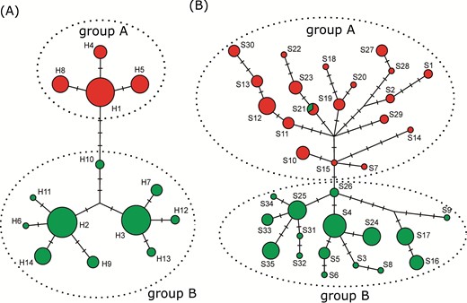
Evolutionary relationships among A. fasciculata DNA sequences. (A) Plastid DNA haplotypes (H1-H14); (B) ITS sequence types (S1-S35). Circle area is proportional to the sequences frequency and perpendicular lines correspond to mutation steps. Haplogroups A and B are indicated.
The ITS dataset produced 35 sequence types (Table 3). The most frequent sequence type was S4, which was detected in 18 individuals from five populations. The sequence type network revealed two main groups that corresponded to the two plastid haplogroups. Only one sequence type (S21), observed in low frequency, was shared among individuals from the two groups. ITS sequences revealed population diversity indices higher than those of the plastid DNA haplogroups; again, populations from group B were more diverse than those from group A and only one population was monomorphic. The genetic groups A and B were strongly supported by BAPS and further demographic results (see next).
Based on plastid DNA data, BAPS analysis (Fig. 3A) found K = 2 to be the best number of groups, recovering the same two groups of populations observed in the networks above. AMOVA (Table 4) based on the plastid dataset indicated a high level of population differentiation (ΦST: 0.95; P < 0.001) with the highest proportion of variation between the two haplogroups (~ 76%). BAPS analysis (Fig. 3B) of ITS data found K = 4 to be the best number of groups, where the two plastid DNA groups were divided into two. In group A, populations Afasc1 to Afasc4 were separated from populations Afasc5 to Afasc7, whereas in group B, population Afasc13 was separated from the others. Only one individual from population Afasc10 grouped in the first subcluster and one individual from population Afasc12 grouped with population Afasc13. In both cases, the small geographical distances may explain the unexpected clustering of individuals. The plastid DNA haplogroups A and B presented a clear north-south distribution. The two ITS subgroups in group A found in BAPS also presented a north-south distribution with the Doce River between them (Fig. 1). The subgroup of group B that consists of only population Afasc13 is located at a lower elevation in the group B (Table 1), although Afasc12 is also in a similar elevation. AMOVA (Table 4) of the ITS data (ΦST = 0.8; P < 0.001) indicated a high level of differentiation, with higher diversity found among populations within groups (~ 53%). The Mantel test showed positive and significant correlation between genetic and geographical distances [r = 0.457 (P < 0.01) based on plastid sequences and r = 0.461 (P < 0.01) for ITS sequences].
AMOVA results based on plastid and nuclear markers for total sampling of A. fasciculata
| Genetic marker | Source of variation | Percentage of variation | ΦST |
|---|---|---|---|
| plastid | among groups | 76.34 | 0.95* |
| among populations | 18.40 | ||
| within populations | 5.25 | ||
| nuclear | among groups | 27.00 | 0.80* |
| among populations | 53.46 | ||
| within populations | 19.54 |
*P < 0.001
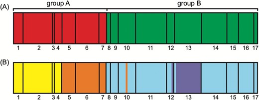
Population genetic structure as inferred through BAPS analysis for A. fasciculata. A, Plastid DNA and B, ITS. Colours indicate groups and populations are numbered: populations 1 to 7 correspond to the A group as observed based on evolutionary relationships of haplotypes and sequence types, respectively, and populations 8 to 17 belong to the B cluster.
The Bayesian inference phylogenetic tree based on concatenated plastid markers plus nuclear sequences revealed two main clades (Fig. 4; Supplementary Information, Fig. S2 for not collapsed branches) that corresponded to Network groups A and B. Full support was observed in clade separation and the estimated age for this split was c. 1.32 Myr (95% HPD; 0.97–1.81 Myr). Clade B diversification started c. 1.0 Mya (0.69–1.42 Mya), whereas diversification in the clade A started 0.71 Mya (0.48–1.06 Mya). Species appearance and internal clade diversification have occurred concomitantly with the Pleistocene (c. 2.6-0.012 Mya).
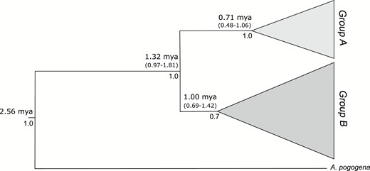
Bayesian inference phylogenetic tree obtained from plastid and nuclear sequences for A. fasciculata. Numbers above branches correspond to mean and intervals age and numbers below the branches are posterior probabilities (PP).
Demography and past distribution
The theta values estimated with Migrate varied among populations and differed between markers (Supplementary Information, Table S4). In general, theta was higher based on ITS than on plastid markers, except in three populations (Afasc4, Afasc8 and Afasc15). On average, theta based on nuclear sequences was higher in group A, whereas based on plastid variability was higher in group B. The extended Bayesian skyline plot (Fig. 5) indicated that the size of A. fasciculata group A showed a population reduction from c. 50 Kya to the present, whereas group B showed an increase in population size around the same period.
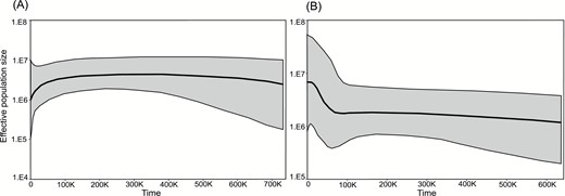
A, B, Population size dynamics over time as investigated using extended Bayesian skyline plots for A. fasciculata genetic group A (A) and genetic group B (B), respectively. Solid areas correspond to confidence intervals.
Ecological niche modelling
Based on the present WorldClim bioclimatic layers, the variables that most contributed to the models were precipitation during the driest month and precipitation seasonality (25.8 and 19.3%, respectively). During the LIG (125 Kya), the ENMs showed an expansion of suitable niches to the north and the south in the BAF. The climate during the LGM (22 Kya) was not suitable for A. fasciculata; however, the restriction imposed by climate conditions was more pronounced for the genetic group B. Some areas in the Amazon Forest were identified as suitable for the species in the LGM. The Mid-Holocene was restrictive to both groups, and their suitable environments were limited and similar to their current areas (Fig. 6). All models showed AUC values > 0.98.
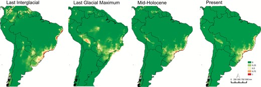
Environmental niche modelling to the past and present A. fasciculata geographical distribution.
The niche overlap values estimated in ENMTools for the genetic groups (Table 5) were significantly smaller (P < 0.05) than those for the null models in the niche identity tests, indicating independence between groups of populations in the past as it happens in the present.
Niche overlapping estimated between the groups A and B of A. fasciculata
| Model | Schoener’s D | I statistic | Relative rank |
|---|---|---|---|
| Last Interglacial | 0.48 | 0.74 | 0.75 |
| Last Glacial Maximum | 0.33 | 0.56 | 0.65 |
| Mid-Holocene | 0.35 | 0.62 | 0.63 |
| Present | 0.58 | 0.82 | 0.76 |
| Model | Schoener’s D | I statistic | Relative rank |
|---|---|---|---|
| Last Interglacial | 0.48 | 0.74 | 0.75 |
| Last Glacial Maximum | 0.33 | 0.56 | 0.65 |
| Mid-Holocene | 0.35 | 0.62 | 0.63 |
| Present | 0.58 | 0.82 | 0.76 |
DISCUSSION
We analysed genetic diversity, population structure, demography and ecological niche modelling of a perennial shrub dispersed throughout the BAF. Different approaches based on genetic, geographical and ecological data indicated that A. fasciculata is divided into two main groups of populations that have originated and diversified during the Pleistocene. We discussed four hypotheses that could explain the genetic diversity of this shrub species that can be considered a key component of BAF. Our results pointed to the BAF refuge theory and climate differences throughout the BAF as the most likely patterns to explain the geographical distribution of genetic variability and structure for A. fasciculata.
The first pattern we tested was a scenario of fragmentation from a previous widely distributed population with a consequent reduction in population connectivity, which would be expected if the rivers that cross the species distribution (e.g. Doce River) were barriers to gene flow, as observed for Passiflora contracta Vitta, where the Paraguassu, Jequitinhonha, Mucuri, and Doce Rivers split the species into five phytogeographical groups (Cazé et al., 2016). Under this scenario, one might expect that the genetic diversity of A. fasciculata would be homogeneously distributed throughout the species range, and divergence between the two clades (groups A and B) would be synchronous. As indicated by the Network results, populations were not structured according to the courses of rivers and the split between both groups did not correspond to any other identified geographical barrier.
In a second scenario, we considered that the ancestral polymorphism could be older than the Pleistocene climate changes, and therefore initial diversification would not have been influenced by glacial and interglacial cycles. Different from what was observed in other species that showed divergence before the last LIG or LGM (e.g. Menezes et al., 2016; Peres et al., 2019) or even that have originated before, during the Pliocene as Passiflora contracta, to then diversify under the Pleistocene climate shifts (Cazé et al., 2016), our dated phylogenetic tree revealed that A. fasciculata has originated and diversified during the Pleistocene, a period of intense shifts in climate and general ecological scenarios (Behling & Negrelle, 2001; Behling, 2002; Ledru et al., 2005), c. 1.3–0.7 Mya, and therefore could have been under influence of these climate changes and sea-level oscillations.
In the third and fourth tested scenarios, we evaluated the refuge hypothesis and ecological differentiation in the BAF as drivers for the origin and diversification of A. fasciculata. In the case of successive rounds of colonization from refugia, the presence of a gradient of genetic diversity would be expected, with gradual differentiation of clades and demographic signs of population expansion and recent colonization, as found for several species from different areas in the BAF (e.g. Carnaval et al., 2014). Moreover, if groups of lineages or populations were associated with different ecological conditions (e.g. D’Horta et al., 2011), we could expect differences in their evolutionary history related or not to the area history, even with different origins and diversification times for these groups. These two scenarios are supported by our main results: suitable ancestral areas coinciding with refugia areas; few evolutionary steps between sequences in each haplogroup or between sequence groups; population expansion at least in the group B; and genetic groups A and B have evolved under different climate drivers as observed based on estimated niche overlapping for both and current climate heterogeneity in the BAF.
The Pleistocene climate changes had a strong impact on BAF shape (Hewitt, 2000) and many plant species were among those that were most influenced (Turchetto-Zolet et al., 2013). The Quaternary refuge hypothesis has been supported by several phylogeographic studies (see the review in Leal et al., 2016) throughout the region. Refuge theory indicates that, during the glaciation periods in South America, forests contracted and persisted only in humid areas because of the drier climate. These moister areas became refugia for humidity-dependent species, and vicariance drove diversification. We observed that A. fasciculata lost suitable area during the LGM, undergoing range fragmentation that should have limited the species occurrence to some known BAF refugia (Carnaval et al., 2014). Similarly to some non-forest species (e.g. Jakob, Martinez-Meyer & Blattner, 2009; Antonelli et al., 2010; Cosacov et al., 2010) and sand-dune plants (e.g. Kadereit et al., 2005; King et al., 2009) from the BAF, we have found only a slight significant impact on the effective size.
Currently, A. fasciculata populations from refuge areas display higher genetic diversity and private polymorphisms compared to other areas, as proposed for other species (Hewitt, 2000). Most studies revealed that source populations show higher levels of variability (Hewitt, 1996; Olsen et al., 2004), whereas the newly colonized areas are expected to harbour a subset of the source gene pools. However, in some species, populations from recently colonized areas are equally or even more diverse than those from refugia (e.g. Olsen et al., 2004; Muellner et al., 2005).
Areas described as refugia for several animal and plant species (Carnaval et al., 2009) coincide with areas in the distribution of A. fasciculata, such as the Bahia (populations Afasc1 and Afasc2) and São Paulo (populations Afasc11, Afasc12 and Afasc13) refugia. The A. fasciculata populations from these areas hosted the highest number of different haplotypes and sequence types, independent of the sampling size, and generally showed exclusive sequences, many of them ancestral to the remaining haplotypes. Some other A. fasciculata populations (Afasc14, Afasc15 and Afasc16) were collected in areas that correspond to the SHG region that is considered as a refuge for several species (Barros et al., 2015), and these populations also showed high diversity indices (h and π). The populations located in the borders of their respective groups had, in general, the lowest diversity.
The populations with haplotypes from the southern haplogroup B, such as those from São Paulo and SHG refugia, diverged before those from haplogroup A, suggesting an expansion from south to north in this species during the Pleistocene, in agreement with other species in the genus (Zamberlan et al., 2015). Although our results should be taken with caution because the estimated age ranges for clades overlap, events of colonization and diversification from south to north in the BAF have been described for several species in Solanaceae (e.g. Reck-Kortmann et al., 2014; Mäder & Freitas, 2019) and other families (e.g. Thode et al., 2014; Teixeira et al., 2016; Turchetto-Zolet et al., 2016).
A high frequency of arboreal pollen is associated with a short dry season and moist climate in low latitudes in the tropics, which could increase the distribution area when the weather is wetter (Ledru, 1993). Highly fragmented areas, in turn, are limiting to dispersion of small mammals such as bats and rodents that include A. fasciculata fruits in their diet, as these animals are dependent on continuous forest fragments (Ferreira et al., 2017). During the Pleistocene, several areas in South America were characterized by valleys that provided a wide range of microhabitats suitable as refugia for forest-adapted taxa (Markgraf, McGlone & Hope, 1995) and their pollinators and dispersers. Moreover, strong winds, predominantly from the east, and the rain shadow effect during pollination and seed dispersion have affected gene flow patterns in several species (e.g. Premoli & Kitzberger, 2005; Arana et al., 2010). These events could be useful to explain, at least in part, the most limited diversity observed for A. fasciculata based on plastid markers, as plastids have mainly maternal inheritance among Solanaceae (Thyssen, Svab & Maliga, 2012).
Additionally, it is suggested that fragmentation under past and present climatic scenarios based on suitability estimates may provide valuable input on range continuity and persistence (Quiroga et al., 2012) and can shed light on the origin of population groups. Our niche modelling analyses draw different scenarios for the two evolutionary groups of A. fasciculata, in agreement with the hypothesis of double origin of the BAF: in the north, derived from the contact zone with the Amazon Forest and, in the south, from the contact area with remaining forests in Argentina and Bolivia (Morley, 2000). The estimated divergence time of the haplogroups is close to the most intense glacial period in South America, the Great Patagonian Glaciation, which promoted the maximum expansion of ice in the region (Rabassa, Coronato & Salemme, 2005) with several ice-free areas remaining (Soliani, Gallo & Marchelli, 2012) from which the haplogroups probably expanded and diversified after the climate got warmer and wetter in the region.
Moreover, the Amazon Forest and BAF are currently separated by the South American dry diagonal. A study based on environmental niche modelling for species from these forests (Sobral-Souza, Lima-Ribeiro & Solferini, 2015) indicated a connection between the northern BAF and western Amazon, and divided the southern BAF in two groups, coastal and countryside, with the last connected to the eastern Amazon. These BAF divisions and connections with the Amazon could have allowed differential diversification of our two clades from different founder effects. Haplogroup A populations are located in the northern BAF, whereas haplogroup B sites are within the southern distribution. The BAF division (Sobral-Souza et al., 2015) agrees with the course of the Doce River and each partition is characterized by particular climate conditions. Our analyses of niche superimposition have demonstrated that each A. fasciculata population group was influenced by different climate variables during the diversification.
Due to its distribution, haplogroup B was probably more affected during the Pleistocene, and the ancestral populations would have been restricted to valleys where environmentally favourable microclimates allowed the establishment of plant patches observed in other species (Antonelli et al., 2009; Antonelli & Sanmartín, 2011). Similar to other species in South America (Pouchon et al., 2018), the climatic cycles during the Pleistocene undoubtedly impacted the adaptation, diversity and distribution of A. fasciculata in periods of connectivity and spatial isolation that gave rise to the two observed distinct evolutionary groups, which diversified in allopatry.
The populations of A. fasciculata are found in remnant patches of the BAF that are currently discontinuous and reduced (Morellato & Haddad, 2000), which may decrease the genetic diversity and impose barriers to gene flow between the haplogroups A and B, increasing their differentiation, as seem from Network and Amova results for both plastid and nuclear markers. These two groups of populations are not related to the presence of geographical barriers, step-stone gene flow, elevation or distance to the sea coast. Instead, these groups seem to be a consequence of the founder effect that, combined with low gene flow, prolonged isolation and long-term persistence, and it is probably a common rule for several plant species from the BAF (e.g. Barbará et al., 2007; Pinheiro et al., 2014; Cazé et al., 2016; Turchetto et al., 2018).
In summary, using a phylogeographic approach to analyse A. fasciculata across its entire current distribution in the BAF, combining molecular information with past niche suitability, we revealed that this species from the Brazilian Atlantic Forest has evolved under the influence of Pleistocene climate changes. Two haplogroups emerged from different refugia and were under different environmental influences, illustrating previously proposed connections between the Atlantic and the Amazon Forests, the two most important Neotropical rainforests.
SUPPORTING INFORMATION
Additional Supporting Information may be found in the online version of this article at the publisher’s web-site:
Table S1. Geographical coordinates used in environmental niche modelling to the past Athenaea fasciculata geographic distribution
Table S2. Pearson Correlation matrix for all pairs of 19 climate variables from WorldClim and 53 sites of occurrence of A. fasciculata
Table S3. Neutrality tests considering total sampling and genetic groups for A. fasciculata
Table S4. Theta values for A. fasciculata populations as estimated per genetic markers
Figure S1. Brazilian Atlantic Forest biome limits records for A. fasciculata.
Figure S2. Bayesian inference phylogenetic tree obtained from plastid and nuclear sequences for A. fasciculata with non-collapsed clades.
ACKNOWLEDGEMENTS
We thank A.M.C. Ramos-Fregonezi, G. Barboza, I. Rodrigues, J.N. Fregonezi, L. Giacomin, P. Viana and V.A. Thode for assistance in the field collections and L. Castro and M.S. Silveira for laboratory assistance. This work was supported by the Conselho Nacional de Desenvolvimento Científico e Tecnológico (CNPq); Coordenação de Aperfeiçoamento de Pessoal de Nível Superior (CAPES); and Programa de Pós-Graduação em Genética e Biologia Molecular—Universidade Federal do Rio Grande do Sul (PPGBM-UFRGS). G. Mäder was supported by PNPD-CAPES/PPGBotanica-UFRGS.
REFERENCES
Author notes
These authors have contributed equally to this work.
