


Summary
The use of social contact rates is widespread in infectious disease modeling since it has been shown that they are key driving forces of important epidemiological parameters. Quantification of contact patterns is crucial to parameterize dynamic transmission models and to provide insights on the (basic) reproduction number. Information on social interactions can be obtained from population-based contact surveys, such as the European Commission project POLYMOD. Estimation of age-specific contact rates from these studies is often done using a piecewise constant approach or bivariate smoothing techniques. For the latter, typically, smoothness is introduced in the dimensions of the respondent’s and contact’s age (i.e., the rows and columns of the social contact matrix). We propose a smoothing constrained approach—taking into account the reciprocal nature of contacts—introducing smoothness over the diagonal (including all subdiagonals) of the social contact matrix. This modeling approach is justified assuming that when people age their contact behavior changes smoothly. We call this smoothing from a cohort perspective. Two approaches that allow for smoothing over social contact matrix diagonals are proposed, namely (i) reordering of the diagonal components of the contact matrix and (ii) reordering of the penalty matrix ensuring smoothness over the contact matrix diagonals. Parameter estimation is done in the likelihood framework by using constrained penalized iterative reweighted least squares. A simulation study underlines the benefits of cohort-based smoothing. Finally, the proposed methods are illustrated on the Belgian POLYMOD data of 2006. Code to reproduce the results of the article can be downloaded on this GitHub repository https://github.com/oswaldogressani/Cohort_smoothing.
1. Introduction
Understanding the spread of infectious diseases in an epidemic context is a challenging task for mathematical modelers. It is especially made difficult by the complexities and intricacies of demography dynamics and rich social contact networks. Social contact mixing patterns play a key role in assessing disease transmission and are known to be crucial determinants of important epidemiological parameters such as the basic reproduction number and the force of infection (see e.g., Vynnycky and White, 2010; Hens and others, 2009). One approach to account for mixing patterns is by the use of the so-called “Who Acquires Infection From Whom” (WAIFW) matrix and the use of serological data to estimate the WAIFW parameters (Anderson and May, 1991; Greenhalgh and Dietz, 1994; Farrington and others, 2001; Van Effelterre and others, 2009). Another approach proposed by Farrington and Whitaker (2005) is to model contact rates as a continuous surface and estimate parameters from serologic survey data. The main limitations of both approaches are that they rely on structural assumptions on the WAIFW matrix and on an arbitrary choice of the parametric model used for the continuous contact surface.
Alternatively, over the last two decades or so, several studies have reported on ways of collecting data on social mixing behavior relevant to the spread of close contact infections directly from individuals through self-reported number of contacts (Wallinga and others, 2006; Beutels and others, 2006; Edmunds and others, 1997; Edmunds and others, 2006; Mikolajczyk and others, 2007). The POLYMOD initiative can arguably be counted among the most important studies in infectious disease epidemiology in Europe, providing large and representative population-based surveys on social contacts (Mossong and others, 2008).
The estimation of smooth age-specific contact rates from the POLYMOD project data is typically performed by applying a negative binomial model on the aggregated number of contacts. To ensure enough flexibility, a bivariate frequentist smoothing method using a tensor product spline is implemented (Mossong and others, 2008; Hens and others, 2009; Goeyvaerts and others, 2010). Estimating social contact rates using the Bayesian paradigm, by means of Gaussian Markov Random Fields using Integrated Nested Laplace Approximations (Rue and others, 2009) as the main tool for inference, has been done as well (van de Kassteele and others, 2017).
The bivariate smoothing approach usually applies smoothing terms in the direction of the respondent’s and contact’s ages of the social contact matrix. However, people age over time and their contact behavior varies smoothly when aging, and applying smoothing terms on the diagonal components (including all subdiagonals) of the social contact matrix would reflect this feature (e.g., the number of contacts between individuals of age |$i$| and |$j$| will be highly related to the number of contacts between individuals 1 year older of age |$i+1$| and |$j+1$|). Note that, in addition, often a steady state (time equilibrium) assumption is made when using social contact data to inform mathematical modeling of infectious diseases meaning that the number of people in different disease states and thus also the rate at which people move states do not depend on time but only on age. This implies that cohorts, i.e., groups of people born in the same year, change disease states with age, and thus leading to a cohort interpretation of the diagonals of the social contact matrix. We opt to smooth from a cohort perspective and propose a new smoothing constrained modeling approach where contact rates are assumed to be smooth over the diagonals (and all subdiagonals) of the social contact matrix. Under the likelihood framework, diagonal smoothing of social contact matrices is achieved through two alternative approaches: (i) reordering of the diagonal components yielding a rectangular grid and (ii) reordering of the penalty matrix to translate a penalization scheme over the diagonal components. Approach (i) builds further upon work published by two of the coauthors in a proceedings paper (Camarda and others, 2013).
The article is organized as follows. Section 2 aims at presenting three competing approaches to smoothly estimate social contact rates. Section 3 investigates the statistical performance of the proposed approaches through a simulation study, and Section 4 illustrates the methodology on the Belgian POLYMOD data. Finally, Section 5 concludes with a discussion and prospects for future research.
2. Smoothing social contact data
In this section, we present the general modeling framework and three competing Smoothing Constrained Approaches (SCAs) to infer social contact rates. First, we describe the classic approach where smoothing is performed in the dimensions of the respondent’s and contact’s ages. The latter baseline model will be referred to as |$\mathcal{M}_0$|. Second, we present the new competing models, namely the SCA where contact rates are assumed smooth from a cohort perspective. Two approaches are investigated both in terms of performance and computational speed, namely model |$\mathcal{M}_1$|, where a reordering of the diagonal components is considered to reproduce a rectangular contact matrix; and model |$\mathcal{M}_2$|, where a reordering of the components of the penalty matrix yields a penalization scheme targeting the diagonal components of the social contact matrix.
2.1. Modeling framework
Let |$\mathbf{Y}=(y_{ij})$| be a square (|$m \times m$|) matrix, where the |$ij$|th entry is the total number of contacts made by the respondents of age |$i-1$| with individuals of age |$j-1$|, with indices |$i=1,\ldots,m$| and |$j=1,\ldots,m$|. This information can be extracted from the self-reported contact diaries of the participants for the Belgian POLYMOD data. Note that for children aged 0–8 years parental proxy reporting was used whereas children aged 9–17 reported contacts themselves as was the case for 18+. For more details, we refer to Supplementary Table 1 in Mossong and others (2008). Furthermore, let the |$m \times 1$| vector |$\mathbf{r}=(r_{i})$| contain the total number of respondents of age |$i-1$|. Define the |$m \times m$| matrix |$\mathbf{E} = \mathbf{r}\mathbf{1}_{m}$|, where |$\mathbf{1}_{m}$| is a |$1 \times m$| vector of ones. Let the |$m \times 1$| vector |$\mathbf{p}=(p_{i})$| denote the population size of individuals of age |$i-1$| and define the |$m \times m$| matrix |$\mathbf{P} = \mathbf{p}\mathbf{1}_{m}$|. Supplementary material available at Biostatistics online provides examples of how to construct these vectors and matrices for the specific case |$m=4$|.
The expected number of contacts made by participants of age |$i-1$| with contacts of age |$j-1$| equals the number of respondents of age |$i-1$| (|$r_{i}$|) multiplied with the average number of contacts an individual of age |$i-1$| makes with an individual of age |$j-1$| (|$\gamma_{ij}$|), thus E|$(y_{ij})=\mu_{ij}=r_{i} \gamma_{ij}$|. The so-called social contact matrix |$\boldsymbol{\Gamma}$| is defined as the |$m \times m$| matrix with elements |$\gamma_{ij}$| (see Figure 1A).
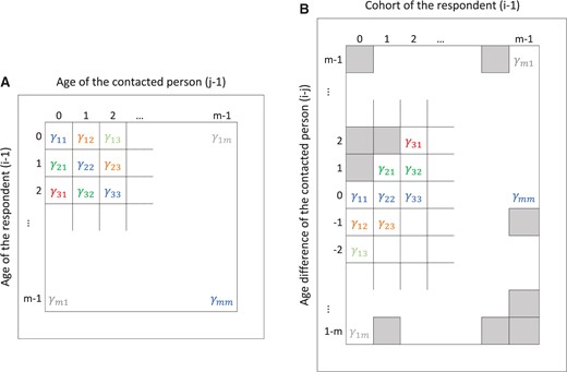
Schematic representation of the original data structure of |$\boldsymbol{\Gamma}$| over ages of respondents and ages of contacts (A) and the restructured matrix |$\breve{\boldsymbol{\Gamma}}$| over cohorts of the respondents and age differences of the contacted persons (B). Cells with nuisance parameters in |$\breve{\boldsymbol{\Gamma}}$| are depicted with gray squares.
Finally, define the |$m^2 \times 1$| vectors |$\mathbf{y}$|, |$\mathbf{e,}$| and |$\boldsymbol{\gamma}$| by arranging |$\mathbf{Y}$|, |$\mathbf{E,}$| and |$\boldsymbol{\Gamma}$| by row order into a vector, respectively. Note that the expected number of contacts can be written as E|$(\mathbf{y})=\boldsymbol{\mu}=\mathbf{e} \odot \boldsymbol{\gamma}$|, where |$\odot$| denotes component-wise multiplication (also known as Hadamard product).
The interest lies in estimating the unknown parameters |$\gamma_{ij}$| from data |$\mathbf{y}$|. Because of the overdispersion in the reported contact counts, we assume that the observed contacts are realizations from a negative binomial distribution, i.e., |$y_{ij} \sim \mbox{NegBin}(\mu_{ij},\alpha_{ij})$|. This implies that |$\mbox{E}({Y_{ij}})=\mu_{ij}$| and |$\mbox{Var}({Y_{ij}}) = \mu_{ij} + \mu_{ij}^2 \alpha_{ij}^{-1}$|. We consider two alternative parameterizations. First, assuming |$\alpha_{ij} = \mu_{ij}\phi^{-1}$|, where |$\phi>0$| denotes the dispersion parameter, implies that the variance is given by |$\mbox{Var}({Y_{ij}})=\mu_{ij}(1+\phi)$|. In the limiting case where |$\phi$| tends to zero, the mean and variance will be equal. Note that the variance term resembles the error term of an overdispersed Poisson distribution, also known as quasi-Poisson (Nelder and Lee, 1992). Second, the alternative parameterization with |$\alpha_{ij}=\phi^{-1}$|, implying that |$\mbox{Var}({Y_{ij}})=\mu_{ij}(1+\phi\mu_{ij})$| was also explored. The first and second parameterizations are further referred to as NB1 and NB2, respectively.
For modeling purposes, a log-link function is specified so that |$\log(\boldsymbol{\mu}) = \log(\mathbf{e})+\log(\boldsymbol{\gamma}) = \log(\mathbf{e})+\boldsymbol{\eta}$|, where |$\log(\boldsymbol{\gamma}) = \boldsymbol{\eta}$|. Let |$\mathbf{H}$| be the |$m \times m$| matrix with |$ij$|th element |$\eta_{ij}$| (the log contact rates). The parameters |$\eta_{ij}$| are penalized (Sections 2.2, 2.3, and 2.4) such that a smooth contact rate surface is obtained. Further, the proposed modeling approach ensures that estimated social contact rates are reciprocal. Reciprocity of contacts means that the total number of contacts on the population level from age |$i$| to age |$j$| must equal the total number of contacts from age |$j$| to age |$i$|.
Reciprocity of contacts can be expressed mathematically as |$\gamma_{ij}p_{i} = \gamma_{ji}p_{j}$|. This can be written as the difference |$\log(\gamma_{ij}) - \log(\gamma_{ji}) = \log(p_{j}) - \log(p_{i})$| and thus:
In matrix form:
where |$\mathbf{L}$| is a |$\frac{m(m-1)}{2} \times m^2$| allocation matrix with entries |$+1$| and |$-1$| to suit the left-hand side of (2.1) and vector |$\boldsymbol{\nu}$| is given by:
In case the dispersion parameter |$\phi$| is fixed, estimation of the parameters |$\boldsymbol{\eta}$| that satisfy the reciprocal constraints is performed through constrained penalized iterative reweighted least squares (C-PIRLS) (Nelder and Wedderburn, 1972; McCullagh and Nelder, 1989; Eilers and Marx, 1996; Wood, 2006). Given current estimates |$\hat{\boldsymbol{\eta}}^{[k]}$| at iteration |$k$|, parameter estimates |$\hat{\boldsymbol{\eta}}^{[k+1]}$| at iteration |$k+1$| are obtained by solving the set of linear equations:
In (2.3), |$\boldsymbol{\zeta}^{[k+1]}$| is a |$\frac{m(m-1)}{2} \times 1$| vector of Lagrange multipliers, |$\mathbf{W}^{[k]}$| is a |$m^2 \times m^2$| diagonal matrix with entries |$W_{ll}^{[k]} = \mu_{l}^{[k]}/(1+\phi)$| (for NB1) and |$W_{ll}^{[k]} = \mu_{l}^{[k]}/(1+\phi\mu_{l}^{[k]})$| (for NB2), |$\mathbf{P}^{*}$| will be introduced in later sections, and |$\mathbf{z}^{[k]}$| is a |$m^2 \times 1$| vector of so-called pseudodata given by:
The parameter estimates |$\hat{\boldsymbol{\gamma}}^{[k+1]}$| are obtained by exponentiation (i.e., |$\hat{\boldsymbol{\gamma}}^{[k+1]} = \exp\big(\hat{\boldsymbol{\eta}}^{[k+1]}\big)$|).
Rather than fixing |$\phi$| at a certain value, the interest is in a data-driven estimate of |$\phi$| as well. For this, a two-stage iteration scheme is undertaken, namely by iterating and cycling between holding |$\phi$| fixed and holding |$\boldsymbol{\eta}$| fixed at its current estimate. More specifically, by holding |$\phi$| fixed at the current estimate |$\hat{\phi}^{[k]}$|, estimates |$\hat{\boldsymbol{\eta}}^{[k+1]}$| are obtained through C-PIRLS. Next, |$\boldsymbol{\eta}$| is fixed at |$\hat{\boldsymbol{\eta}}^{[k+1]}$| and an updated estimate |$\hat{\phi}^{[k+1]}$| is obtained using the moment estimator (Breslow, 1984). This process is iterated until convergence. Moment estimation of |$\phi$| is based on the Pearson’s chi-squared statistic (Breslow, 1984), namely:
where |$\widehat{\rm ED}$| is the trace of the matrix given in (2.10). This leads to a straightforward estimate of |$\hat{\phi}^{[k]}$|:
For NB2, the denominator of the left-hand side of (2.5) is |$(1 + \phi \mu_{ij}^{[k]})\mu_{ij}^{[k]}$|. The updated estimate of |$\hat{\phi}^{[k]}$| can be obtained by a root-finding algorithm.
The above iterative process is repeated until convergence, namely until |$\max \mid \hat{\boldsymbol{\eta}}^{[k+1]} - \hat{\boldsymbol{\eta}}^{[k]} \mid < 10^{-4}$| and |$\mid \hat{\phi}^{[k+1]} - \hat{\phi}^{[k]} \mid < 10^{-4}$|.
2.2. Absence of smoothing over cohorts (|$\mathcal{M}_0$|)
Smoothing of the contact rates is performed in the dimensions of the respondent’s and contact’s ages (vertical and horizontal dimension, respectively, of the matrix in Figure 1A). For this, a second-order difference penalty (Eilers and Marx, 1996) is assumed between adjacent log contact rates |$\eta_{ij}$|. The penalty in the horizontal dimension is therefore given by:
This implies that a log contact rate is penalized by its two preceding (|$\eta_{i,j-2}$|, |$\eta_{i,j-1}$|) and succeeding (|$\eta_{i,j+1}$|, |$\eta_{i,j+2}$|) log contact rates. The penalty in the vertical dimension is created in a similar manner.
Using this second-order penalty (2.7) for the horizontal and vertical direction, the penalty term |$\mathbf{P}^{*}$| in (2.3) is a |$m^2 \times m^2$| matrix given by (see Marx and Eilers, 2005):
where |$\otimes$| denotes the Kronecker product and |$\lambda_1$| and |$\lambda_2$| are smoothing parameters for, respectively, the horizontal and vertical dimension in Figure 1A. The matrices |$\mathbf{D}_h$| and |$\mathbf{D}_v$| are second-order difference matrices, and |$\mathbf{I}$| is the identity matrix.
The optimal smoothing parameters |$\lambda_1$| and |$\lambda_2$| are chosen based on minimization of the Akaike Information Criterion (AIC) (Akaike, 1973) via grid search:
where |$\hat{L}$| is the maximized value of the likelihood function and the effective degrees of freedom, |$\widehat{\rm ED}$|, is the trace of the hat matrix given by (see Wood, 2006):
Note that adding 1 to |$\widehat{\rm ED}$| accounts for the estimation of the overdispersion parameter |$\phi$|.
In addition, the Bayesian Information Criterion (BIC) (Schwarz, 1978) is calculated, namely:
Note that for the AIC the effective degrees of freedom are less penalized than in BIC. Therefore, a less smooth model (higher degrees of freedom) is preferred for AIC, whereas the BIC selects a smoother surface (lower degrees of freedom).
2.3. Cohort smoothing by reordering the contact matrix (|$\mathcal{M}_1$|)
We now describe a new approach where contact rates are smoothed over the diagonal components (and all subdiagonals) and thus smoothing from a cohort perspective. For example, assuming again a second-order difference penalty implies that the contact rate |$\gamma_{ii}$| is penalized by the two preceding contact rates |$\gamma_{i-2,i-2}$| and |$\gamma_{i-1,i-1}$|, and the two succeeding contact rates |$\gamma_{i+1,i+1}$| and |$\gamma_{i+2,i+2}$|. Note that in approach |$\mathcal{M}_0$|, the contact rate |$\gamma_{ii}$| is not penalized by other values on the diagonal.
The smoothing over the dimension of the contact’s age is kept, since the distribution of the age of (grand)parents can in general be assumed smooth (e.g., children will meet their parents and grandparents who are, e.g., |$\pm$| 30 and |$\pm 60$| years older). Thus, the contact rate |$\gamma_{ij}$| is penalized by the contact rates |$\gamma_{i,j-2}$|, |$\gamma_{i,j-1}$|, |$\gamma_{i,j+1}$|, and |$\gamma_{i,j+2}$|. We describe how this can be achieved by restructuring the data and contact matrix over the cohorts and the contacts’ ages.
For this purpose, the contact matrix |$\boldsymbol{\Gamma}$| is restructured in such a way that each diagonal (the main diagonal and all subdiagonals) is present as a row in the restructured matrix. A graphical representation of this restructured matrix is given in Figure 1B. The restructured matrix |$\breve{\boldsymbol{\Gamma}}$| has dimension |$(2m-1) \times m$| and is constructed by entering row |$i$| of |$\boldsymbol{\Gamma}$| in column |$i$| of |$\breve{\boldsymbol{\Gamma}}$| at positions |$m-i+1$| to |$2m-i$|. In that manner, all subsequent (sub)diagonal elements are present in the same row.
By construction, matrix |$\breve{\boldsymbol{\Gamma}}$| contains nuisance contact rate parameters that are not of interest (gray squares in Figure 1B). A weight matrix will be included in the estimation step (see below), to avoid that these nuisance parameters influence parameter estimation. We note that the nuisance parameters will also not be included in the calculation of the effective degrees of freedom.
Restructured matrices |$\breve{\mathbf{Y}}$| and |$\breve{\mathbf{E}}$|, are created from |${\mathbf{Y}}$| and |${\mathbf{E}}$| similarly as |$\breve{\boldsymbol{\Gamma}}$|. Missing cell entries are present for |$\breve{\mathbf{Y}}$| and |$\breve{\mathbf{E}}$| at the same cells where the nuisance parameters are present for |$\breve{\boldsymbol{\Gamma}}$|. To handle these missing entries, we impute arbitrary values (e.g., 9999) in |$\breve{\mathbf{Y}}$| and |$\breve{\mathbf{E}}$| and construct a |$(2m-1) \times m$| weight matrix |$\breve{\mathbf{W}}$|, where the |$ij$|th entry of |$\breve{\mathbf{W}}$| equals zero if the |$ij$|th entry in |$\breve{\boldsymbol{\Gamma}}$| is a nuisance parameter and equals one otherwise.
For parameter estimation, define |$\breve{\mathbf{y}}$|, |$\breve{\mathbf{e}}$|, |$\breve{\mathbf{w,}}$| and |$\breve{\boldsymbol{\gamma}}$| be the |$(2m^2-m) \times 1$| vectors obtained by arranging the matrices |$\breve{\mathbf{Y}}$|, |$\breve{\mathbf{E}}$|, |$\breve{\mathbf{W,}}$| and |$\breve{\boldsymbol{\Gamma}}$| by column order into a vector. We have that |$\mbox{E}(\breve{\mathbf{y}}) = \breve{\boldsymbol{\mu}} = \breve{\mathbf{e}} \odot \breve{\boldsymbol{\gamma}} \odot \breve{\mathbf{w}}$|. The reciprocity assumption of the contacts, can again be written in matrix form as |$\mathbf{L} \breve{\boldsymbol{\eta}} = \boldsymbol{\nu}$|, where |$\mathbf{L}$| is an |$(\frac{m(m-1)}{2}) \times (2m^2-m)$| allocation matrix to accommodate the reciprocity constraints.
Estimation of the smoothed parameters |$\breve{\boldsymbol{\eta}}$| is again performed through C-PIRLS. Updated parameter estimates are obtained by solving the set of linear equations given in (2.3), where |$\boldsymbol{\eta}$| is replaced by |$\breve{\boldsymbol{\eta}}$|. Further, we now have that |$\mathbf{W}^{[k]}$| is an |$(2m^2-m) \times (2m^2-m)$| diagonal matrix with entries |$W_{ll}^{[k]} = \breve{\mu}_{l}^{[k]}/(1+\phi)$| (for NB1) and |$W_{ll}^{[k]} = \breve{\mu}_{l}^{[k]}/(1+\phi\breve{\mu}_{l}^{[k]})$| (for NB2) and |$\mathbf{z}^{[k]}$| is an |$(2m^2-m) \times 1$| vector of pseudovalues given by:
Although |$2m^2-m$| parameters |$\breve{\boldsymbol{\eta}}$| are estimated in this case, the interest is only in the |$m^2$| parameters of |$\breve{\boldsymbol{\eta}}$| corresponding to the non-nuisance parameters.
Again, a second-order difference penalty is assumed between adjacent log contact rates in the horizontal and vertical direction of Figure 1B. Therefore, the |$(2m^2-m) \times (2m^2-m)$| penalty matrix |$\mathbf{P}^{*}$| is:
where |$\lambda_1$| and |$\lambda_2$| are smoothing parameters for, respectively, the vertical and horizontal dimension in, i.e., age and cohort of the original data structure.
Due to the inclusion of the weight matrix |$\breve{\mathbf{W}}$| the nuisance parameters do not contribute in the calculation of the effective degrees of freedom (i.e., all nuisance parameters contribute a value of 0 in effective degrees of freedom).
2.4. Cohort smoothing by reordering the penalty matrix (|$\mathcal{M}_2$|)
The second approach to smooth from a cohort perspective is to rearrange the penalty matrix in such a manner that smoothing is performed on the diagonal elements (and all subdiagonals) of the contact matrix. The contact matrix itself is not rearranged and thus has the form of the Figure 1A.
The methodology is similar as described in Section 2.1. The |$m^2 \times m^2$| penalty matrix |$\mathbf{P}^{*}$| is given by:
where |$\lambda_{1}$| and |$\lambda_{2}$| are smoothing parameters for, respectively, the horizontal (smoothing in the dimension of the contact’s ages) and the diagonal dimension in Figure 1A. The |$m^2 \times m^2$| matrix |$\mathbf{P}_{d}^{*}$| is responsible for the penalization of the contact rates in the diagonal (and subdiagonal) direction. Thus, similar as in Section 2.3, the contact rate |$\gamma_{ii}$| is penalized by the two preceding contact rates |$\gamma_{i-2,i-2}$| and |$\gamma_{i-1,i-1}$|, and the two succeeding contact rates |$\gamma_{i+1,i+1}$| and |$\gamma_{i+2,i+2}$|.
The penalty matrix |$\mathbf{P}_{d}^{*}$| is less trivial to construct and has no easy mathematical formulation. An algorithmic approach is needed for the construction of |$\mathbf{P}_{d}^{*}$|. For example, in the specific case where |$\boldsymbol{\Gamma}$| is a |$4 \times 4$| matrix (i.e., |$\boldsymbol{\gamma} = \left\lbrace \gamma_{11}, \gamma_{12}, \gamma_{13}, \gamma_{14}, \gamma_{21}, \ldots, \gamma_{44} \right\rbrace$|), the penalty matrix |$\mathbf{P}_{d}^{*}$| is a |$16 \times 16$| matrix (see Section A of the supplementary material available at Biostatistics online).
A major advantage of using the penalty matrix |$\mathbf{P}_{d}^{*}$| to achieve smoothing from a cohort perspective is the absence of nuisance parameters in the matrix |$\boldsymbol{\Gamma}$| (cf. the approach in the previous section using |$\breve{\boldsymbol{\Gamma}}$|). This is a non-negligible computational gain, since only |$m^2$| parameters in |$\boldsymbol{\Gamma}$| need to be estimated, whereas the |$\mathcal{M}_1$| approach requires estimation of |$2m^2-m$| parameters in |$\breve{\boldsymbol{\Gamma}}$| (and thus including |$m(m-1)$| nuisance parameters).
2.5. Kink on the main diagonal of the social contact matrix
The use of smoothing approaches for estimating social contact rates can lead to estimates that are oversmoothed for individuals of the same age, meaning that the estimated contact rate is smaller than the true one in the population. For example, students make an above average number of contacts with individuals of their own age (e.g., in school, sport clubs, etc.). Smoothing approaches thus, potentially, lead to an underestimation of the social contact rates on the main diagonal of the contact matrix, especially for children and young adults. To take this into account, we introduce the use of a so-called kink on the main diagonal of the social contact matrix for |$\mathcal{M}_1$| and |$\mathcal{M}_2$|. The kink allows for a sudden increase (or decrease) of the estimated social contact rates for children and young adults of the same age.
The kink is introduced through a small adjustment in the penalty matrices (2.13) and (2.14). More specifically, in the dimension of the contact’s age, the social contact rates that belong to the main diagonal, i.e., |$\eta_{ii}$| and |$\gamma_{ii}$|, are not penalized. In (2.13), this is achieved by changing the |$(2m-3) \times (2m-1)$| matrix |$\mathbf{D}_v$| as follows:
From the above matrix |$\mathbf{D}_v^{*}$|, it is clear that the social contact rates that belong to the main diagonal, namely, |$\eta_{ii}$| and |$\gamma_{ii}$|, are not penalized since column |$m$| only has zero values. The penalty matrix in (2.13) is now reformulated as follows:
where |$\mathbf{I}_{m}^{(1)}$| and |$\mathbf{I}_{m}^{(2)}$| are diagonal indicator matrices given by:
where max.kink.age indicates the maximum age at which a kink on the main diagonal is possible. In penalty matrix (2.14), a similar adjustment is applied to the matrix |$\mathbf{D}_h$|.
Here, we calibrate max.kink.age = 31 (i.e., |$\lbrace 0,\ldots,30 \rbrace$| years). A sensitivity analysis with higher values for max.kink.age yielded quantitatively similar results.
It is worth noting that social contact rates on the main diagonal that are adjusted by the kink are still penalized in the diagonal dimension and thus smooth contact rates are obtained on the diagonals of the contact matrix. Models |$\mathcal{M}_{1}$| and |$\mathcal{M}_{2}$| offer a mathematical convenient way to allow for this kink and still allow for parameter penalization over the main diagonal. This is, by design, not achievable with model |$\mathcal{M}_{0}$|. The kink as defined above, acts through an adjustment of the penalty matrix such that main diagonal parameters are only penalized in the diagonal dimension, and not penalized in the horizontal and vertical directions. Such a penalization scheme is incompatible with |$\mathcal{M}_{0}$| as it would lead to main diagonal parameters that are not penalized at all.
Finally, we note that the introduction of this kink in |$\mathcal{M}_{1}$| and |$\mathcal{M}_{2}$| leads to a smoothed contact surface that is nondifferentiable on the main diagonal in the dimension of the contact’s age.
2.6. Quantifying the uncertainty of estimates
In order to quantify the uncertainty of the estimate |$\hat{\boldsymbol{\eta}}$|, we need to compute its associated variance–covariance matrix. For this purpose, we follow Wood (2006) and use a Bayesian approach to determine the posterior variance–covariance matrix by:
Moreover, as justified by large sample results, the corresponding posterior distribution is taken to be multivariate normal:
The above (approximate) posterior distribution can be used to calculate confidence intervals for parameters |$\eta_{ij}$| or for nonlinear functions of these parameters (such as |$\gamma_{ij}$|). An estimate of |$\mathbf{V}_{\boldsymbol{\eta}}$| can be obtained by plugging in |$\mathbf{W}$| at convergence together with the estimated optimal smoothing parameters |$\hat{\lambda}_{1}$| and |$\hat{\lambda}_{2}$| in |$\mathbf{P}^{*}$|.
The result in (2.17) can be used to generate social contact matrices by sampling from the obtained multivariate Gaussian distribution. This can be useful to acknowledge the variability originating from social contact data in the estimation of epidemiological parameters and/or health economic evaluations (Bilcke and others, 2011). Further computational and algorithmic considerations related to C-PIRLS are given in Section B of the supplementary material available at Biostatistics online.
3. Simulation study
A comparison of the methods introduced in Section 2 is implemented via a simulation study. We investigate both a scenario in which no kink is needed on the main diagonal, and a scenario in which a kink is specified. In the simulation study, the NB1 distribution will be considered.
3.1. Simulation setup
Our data-generating process is based on a so-called true social contact matrix, denoted by |$\boldsymbol{\Gamma}^{*}$|, from which data are simulated. To obtain such a matrix, a nonparametric regression is applied to the Belgian social contact data. More specifically, the observed contacts rates (see Figure 2B), |$y_{ij}/r_{i}$| are smoothed using local linear regression. Using a local linear regression approach, there is no guarantee that |$\mathbf{K}^{*} \equiv \boldsymbol{\Gamma}^{*} \odot \mathbf{P}$| is symmetric. Therefore, we derive a symmetric matrix from |$\mathbf{K}^{*}$|, denoted by |$\tilde{\mathbf{K}}^{*}$|, computed as |$ \left( \tilde{\mathbf{K}}^{*} \right)_{ij} = \left( \tilde{\mathbf{K}}^{*} \right)_{ji} = \frac{ \left( \mathbf{K}^{*} \right)_{ij} + \left( \mathbf{K}^{*} \right)_{ji}}{2}. $| The true contact surface, |$\tilde{\boldsymbol{\Gamma}}^{*}$| that is used for data simulation is obtained by |$ \tilde{\Gamma}^{*}_{ij} = \tilde{K}^{*}_{ij} / P_{ij} $|. Finally, we denote the log-transformed matrix by |${H}^{*}_{ij} = \log\left( \tilde{\Gamma}^{*}_{ij} \right)$|.

The number of respondent per age (A) and the observed log-contact rates (|$\log(y_{ij}/r_{i})$|) (B) of the Belgian social contact data. A white cell indicates that there were no contacts observed for those particular ages of the respondents and contacts.
In Figure 3, the true social contact matrices used to generate the data for the simulation study |$\tilde{\boldsymbol{\Gamma}}^{*}$| and |$\mathbf{H}^{*}$| are shown. To account for a kink in the simulation study, we proceed as follows. Let |$\tilde{\boldsymbol{\Gamma}}^{\dagger}$| denote the true social contact matrix with a kink on the main diagonal. Matrix |$\tilde{\boldsymbol{\Gamma}}^{\dagger}$| is similar as matrix |$\tilde{\boldsymbol{\Gamma}}^{*}$|, with the exception that the values of |$\tilde{\Gamma}^{\dagger}_{ii}$|, for |$i=1,\ldots,24$|, are artificially increased in the following manner:
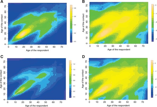
True social contact matrices |$\tilde{\boldsymbol{\Gamma}}^{*}$| (A and C) and |$\mathbf{H}^{*}$| (B and D) without a kink (A and B) and with kink (C and D) used for the data-generating process in the simulation study. The true social contact surfaces are obtained from a nonparametric regression using a local linear fit to the Belgian social contact data.
Thus, for ages between 0 and 23 a higher number of contacts is obtained on the main diagonal. Data are simulated using the same participant distribution as in the Belgian social contact data with sample size |$n=745$| (see Figure 2A). The observed number of contacts are simulated from the NB1 distribution (with |$\phi=2$|):
We simulate |$S=100$| data sets for each setting and fit models |$\mathcal{M}_0$|, |$\mathcal{M}_1$|, and |$\mathcal{M}_2$| without kink, and models |$\mathcal{M}_1$| and |$\mathcal{M}_2$| with kink to each data set. This yields estimated social contact matrices |$\hat{\boldsymbol{\Gamma}}^{(s)}$| and |$\hat{\mathbf{H}}^{(s)}$|, for |$s=1,\ldots,S$|. The estimation performance of the different methods are compared using the squared bias and mean square error (MSE). These scalar measures of performance are given by:
with similar definitions for |$\mbox{Bias}^{2}_{H}$| and |$\mbox{MSE}_{H}$|.
Besides the performance of pointwise estimators, we also assess the accuracy with which uncertainty is quantified by looking at the coverage performance of |$95\%$| pointwise confidence intervals (CIs) of |$\eta_{ij}$|. Using the approximate posterior distribution in (2.17), 95|$\%$| pointwise CIs are easily calculated (i.e., |$\pm 1.96 \times$| the square root of the Bayesian posterior variance). The reported nominal coverages of the CIs are calculated by averaging over all entries of the social contact matrix.
3.2. Simulation results
Results for the squared bias and MSE are presented in Tables 1 and 2, respectively. For all settings, we observe that models that smooth over cohorts (|$\mathcal{M}_1$| and |$\mathcal{M}_2$|) are performing better in terms of MSE than |$\mathcal{M}_0$|, and this holds for both |$\mathbf{H}^{*}$| and |$\breve{\boldsymbol{\Gamma}}^{*}$|. The squared bias results are somewhat less clear, but overall model |$\mathcal{M}_2$| is performing better. When comparing models |$\mathcal{M}_1$| and |$\mathcal{M}_2$|, we observe that the latter model has better performance.
Squared bias of the social contact matrices |$\mathbf{H}^{*}$|and |$\breve{\boldsymbol{\Gamma}}^{*}$|over |$S=100$|simulations using |$\mathcal{M}_0, \mathcal{M}_1$|and |$\mathcal{M}_2$|with and without a kink on the main diagonal
| Squared bias | Models without kink on main diagonal | |||||
|---|---|---|---|---|---|---|
| bias|$^{2}$| of |$\mathbf{H}^{*}$| (|$\mathbf{H}^{\dagger}$|) | bias|$^{2}$| of |$\breve{\boldsymbol{\Gamma}}^{*}$| (|$\breve{\boldsymbol{\Gamma}}^{\dagger}$|) | |||||
| Simulation setting | |$\mathcal{M}_0$| | |$\mathcal{M}_1$| | |$\mathcal{M}_2$| | |$\mathcal{M}_0$| | |$\mathcal{M}_1$| | |$\mathcal{M}_2$| |
| Without kink | 93.16 | 91.53 | 77.76 | 2.50 | 2.63 | 2.52 |
| With kink | 96.52 | 82.14 | 70.44 | 4.77 | 4.38 | 4.31 |
| Squared bias | Models with kink on main diagonal | |||||
| bias|$^{2}$| of |$\mathbf{H}^{*}$| (|$\mathbf{H}^{\dagger}$|) | bias|$^{2}$| of |$\breve{\boldsymbol{\Gamma}}^{*}$| (|$\breve{\boldsymbol{\Gamma}}^{\dagger}$|) | |||||
| Simulation setting | |$\mathcal{M}_0$| | |$\mathcal{M}_1$| | |$\mathcal{M}_2$| | |$\mathcal{M}_0$| | |$\mathcal{M}_1$| | |$\mathcal{M}_2$| |
| Without kink | – | 93.64 | 79.42 | – | 3.05 | 2.92 |
| With kink | – | 80.70 | 68.63 | – | 2.62 | 2.53 |
Mean square error of the social contact matrices |$\mathbf{H}^{*}$|and |$\breve{\boldsymbol{\Gamma}}^{*}$|over |$S=100$|simulations using |$\mathcal{M}_0, \mathcal{M}_1$|and |$\mathcal{M}_2$|with and without a kink on the main diagonal
| MSE | Models without kink on main diagonal | |||||
|---|---|---|---|---|---|---|
| MSE of |$\mathbf{H}^{*}$| (|$\mathbf{H}^{\dagger}$|) | MSE of |$\breve{\boldsymbol{\Gamma}}^{*}$| (|$\breve{\boldsymbol{\Gamma}}^{\dagger}$|) | |||||
| Simulation setting | |$\mathcal{M}_0$| | |$\mathcal{M}_1$| | |$\mathcal{M}_2$| | |$\mathcal{M}_0$| | |$\mathcal{M}_1$| | |$\mathcal{M}_2$| |
| Without kink | 154.73 | 130.41 | 123.72 | 4.79 | 3.99 | 3.96 |
| With kink | 156.94 | 123.59 | 120.50 | 7.11 | 5.86 | 5.87 |
| MSE | Models with kink on main diagonal | |||||
| MSE of |$\mathbf{H}^{*}$| (|$\mathbf{H}^{\dagger}$|) | MSE of |$\breve{\boldsymbol{\Gamma}}^{*}$| (|$\breve{\boldsymbol{\Gamma}}^{\dagger}$|) | |||||
| Simulation setting | |$\mathcal{M}_0$| | |$\mathcal{M}_1$| | |$\mathcal{M}_2$| | |$\mathcal{M}_0$| | |$\mathcal{M}_1$| | |$\mathcal{M}_2$| |
| Without kink | – | 133.15 | 126.00 | – | 4.57 | 4.51 |
| With kink | – | 122.71 | 119.25 | – | 4.41 | 4.40 |
In the simulation settings in which no kink is introduced on the main diagonal, we observe that models with a kink on the main diagonal perform slightly worse than those without a kink. However, in the simulation settings with a kink, a more pronounced difference is observed in favor of the models with a kink on the main diagonal, especially for |$\breve{\boldsymbol{\Gamma}}^{*}$|. The better performance of models including a kink is mainly due to the better estimation of the main diagonal components of the social contact matrix. No meaningful differences are observed outside the main diagonal region.
In general, the overdispersion parameter |$\phi$| is estimated well across all simulation settings. For example, in the simulation setting without a kink, model |$\mathcal{M}_2$| without a kink has an average estimate for |$\phi$| of 1.92 with 95|$\%$| of the estimated overdispersion parameters between 1.74 and 2.22. For the simulation setting with a kink, we have 1.93 (1.71–2.20) for model |$\mathcal{M}_2$| with a kink.
Table 3 highlights the nominal coverage results for |$\mathbf{H}^{*}$| (|$\mathbf{H}^{\dagger}$|) for the different settings. We observe that all models produce pointwise CIs with close to 95|$\%$| nominal coverage. In the simulation setting with a kink, a slight overcoverage is observed for models |$\mathcal{M}_1$| and |$\mathcal{M}_2$|. In this latter scenario, the average lengths of the 95|$\%$| CIs are 0.65, 0.61, and 0.60, for |$\mathcal{M}_0$| without a kink, |$\mathcal{M}_1$| with a kink and |$\mathcal{M}_2$| with a kink, respectively. This implies that the overcoverage is not directly associated with wider CIs. The results in Table 3 indicate that the large sample result in (2.17) can be used to construct CIs with appropriate nominal coverage.
Nominal coverage of 95|$\%$|pointwise confidence intervals of the social contact matrices |$\mathbf{H}^{*}$||$(\mathbf{H}^{\dagger})$|over |$S=100$|simulations using |$\mathcal{M}_0, \mathcal{M}_1$|, and |$\mathcal{M}_2$|with and without a kink on the main diagonal. The nominal coverage is calculated by averaging over the entire social contact matrix
| Models without kink | Models with kink | |||||
|---|---|---|---|---|---|---|
| on main diagonal | on main diagonal | |||||
| Simulation setting | |$\mathcal{M}_0$| | |$\mathcal{M}_1$| | |$\mathcal{M}_2$| | |$\mathcal{M}_0$| | |$\mathcal{M}_1$| | |$\mathcal{M}_2$| |
| Without kink | 95.10 | 94.51 | 95.92 | – | 93.90 | 95.36 |
| With kink | 95.01 | 96.26 | 97.26 | – | 96.22 | 97.26 |
4. Application: Belgian social contact data
The proposed smoothing methods are illustrated on the POLYMOD social contact data of Belgium, obtained through a population-based contact survey carried out over the period of March to May 2006. Participants kept a paper diary with information on their contacts over 1 day. A contact was defined as a two-way conversation of at least three words in each other’s proximity. The gathered information included the age of the contact, gender, location, duration, frequency, and whether or not touching was involved. Sampling weights—the inverse of the probability that a participant is included because of the sampling design—are based on official age and household size data of the year 2000 census published by Eurostat (Mossong and others, 2008). These sampling weights are included in the analysis.
We consider the contact data of all participants aged between 0 and 76 years (both included). We also restrict to contacts made with individuals between 0 and 76 years (both included). Thus, |$m=77$|. In total, we have information on 745 participants with 399 (53.6|$\%$|) females and 345 (46.3|$\%$|) males (one participant with missing sex information). The mean age of the participants is 31 years. A total of 13 493 contacts were reported, giving a crude mean of 18.1 contacts per participant. The age structure of the general population in which the contact survey is conducted in 2006 is obtained from Eurostat (2017), where the population size in the 0–76 years interval is |$N = 9~777~488$|.
Let |$w^{*}_{k}$| denote the normalized sampling weight of participant |$k$|, with |$k=1,\dots,745$|. The |$ij$|th input of |$\mathbf{Y}$| is |$y_{ij} = \sum_{k \ \in \ \mbox{age}_{i-1}} w^{*}_{k} \times \#contacts_{k,j-1}$| and corresponds to a weighted sum of the number of contacts made by respondents of age |$i-1$| with contacts of age |$j-1$|. Similarly, the inputs of the vector |$\mathbf{r}$| are given by |$r_{i} = \sum_{k \ \in \ \mbox{age}_{i-1}} w^{*}_{k}$|. In Figure 2B, the observed log-contact rates |$\log(y_{ij}/r_{i})$| are shown.
Social contact rates are estimated applying models |$\mathcal{M}_0$|, |$\mathcal{M}_1$|, and |$\mathcal{M}_2$| using both NB1 and NB2 distributional assumption. For |$\mathcal{M}_1$| and |$\mathcal{M}_2$|, both models with and without a kink are investigated. Table 4 provides the summary results of the fitted models.
Summary results of the fitted models to the Belgian social contact data. Optimal smoothing parameters, effective degrees of freedom, |$-2\log(\hat{L})$|, AIC, BIC, |$\phi,$|and computational time in seconds (T) are provided
| Model | |$\hat{\lambda_{1}}$| | |$\hat{\lambda_{2}}$| | |$\widehat{\rm ED}$| | |$-2\log(\hat{L})$| | AIC | BIC | |$\hat{\phi}$| | T (s) |
|---|---|---|---|---|---|---|---|---|
| Without kink | ||||||||
| |$\mathcal{M}_0$| NB1 | 15.17 | 16.64 | 181.5 | 20 732.7 | 21 097.7 | 22 318.0 | 3.08 | 93.7 |
| |$\mathcal{M}_0$| NB2 | 4.56 | 4.56 | 318.0 | 20 355.3 | 20 993.2 | 23 126.6 | 1.49 | 118.6 |
| |$\mathcal{M}_1$| NB1 | 22.76 | 1714.91 | 55.8 | 20 988.5 | 21 102.1 | 21 481.8 | 3.76 | 238.8 |
| |$\mathcal{M}_1$| NB2 | 4.16 | 5.0 | 307.0 | 20 471.6 | 21 087.6 | 23 147.5 | 1.59 | 377.2 |
| |$\mathcal{M}_2$| NB1 | 27.36 | 1564.02 | 59.5 | 20 994.2 | 21 115.2 | 21 519.5 | 3.76 | 50.5 |
| |$\mathcal{M}_2$| NB2 | 4.16 | 5.48 | 317.1 | 20 471.4 | 21 107.6 | 23 235.0 | 1.59 | 88.4 |
| With kink | ||||||||
| |$\mathcal{M}_1$| NB1 | 30.00 | 1584.89 | 54.3 | 20 967.6 | 21 078.2 | 21 448.2 | 3.70 | 239.4 |
| |$\mathcal{M}_1$| NB2 | 4.37 | 5.25 | 303.4 | 20 473.1 | 21 081.8 | 23 117.2 | 1.60 | 375.6 |
| |$\mathcal{M}_2$| NB1 | 40.00 | 1584.89 | 55.4 | 20 973.2 | 21 086.0 | 21 463.4 | 3.70 | 48.4 |
| |$\mathcal{M}_2$| NB2 | 4.56 | 5.48 | 313.2 | 20 472.8 | 21 101.2 | 23 202.4 | 1.60 | 85.4 |
It is observed that model |$\mathcal{M}_0$| with the NB2 distribution provides the lowest AIC value (smaller AIC is better). Whereas for the BIC, the lowest values are observed for the NB1 distribution and using models |$\mathcal{M}_1$| and |$\mathcal{M}_2$| both with kink. For both NB1 and NB2, it is observed that models |$\mathcal{M}_1$| and |$\mathcal{M}_2$| with kink have lower AIC and BIC values than models |$\mathcal{M}_1$| and |$\mathcal{M}_2$| without kink. All models with the NB2 distribution have higher effective degrees of freedom (|$\widehat{\rm ED}$| from 303.4 to 318.0) than the NB1 distribution models. For NB1, |$\mathcal{M}_{0}$| has higher effective degrees of freedom (|$\widehat{\rm ED}=181.5$|) than models |$\mathcal{M}_1$| and |$\mathcal{M}_2$| (|$\widehat{\rm ED}$| from 54.3 to 55.4). From here, we focus on the results of the NB1 distribution since these models have smoother surfaces.
Regarding the estimated smoothing parameters |$\hat{\lambda}_{1}$| and |$\hat{\lambda}_{2}$|, an interesting difference is observed between |$\mathcal{M}_0$| and models |$\mathcal{M}_1$| and |$\mathcal{M}_2$|. In |$\mathcal{M}_0$|, the optimal values for |$\hat{\lambda}_{1}$| and |$\hat{\lambda}_{2}$| are of similar magnitude, while for the models accounting for cohort smoothing, the optimal value for |$\hat{\lambda}_{2}$| is larger than |$\hat{\lambda}_{1}$|, indicating that more penalization is performed in the direction of the cohorts.
In terms of computational speed, fitting model |$\mathcal{M}_2$| is approximately 4 times faster as compared to model |$\mathcal{M}_1$|, as for the latter model |$2m^2-m=11~781$| parameters (including |$m^2-m$| nuisance parameters) need to be estimated, as compared to |$m^2=5929$| parameters for |$\mathcal{M}_2$|. It is also observed that fitting models |$\mathcal{M}_2$| is somewhat faster than |$\mathcal{M}_{0}$|.
In Figure 4, the estimated log contact rate surfaces, |$\hat{\mathbf{H}}$| for models |$\mathcal{M}_0$|, |$\mathcal{M}_1$| without a kink, and |$\mathcal{M}_2$| without a kink are shown for NB1. The figures for the mixing at the population level, |$\hat{\boldsymbol{\Gamma}} \odot \mathbf{P}$|, are provided in the supplementary material available at Biostatistics online (Figure 2). Generally, the surfaces are able to capture important features of human contact behavior. There is a clear difference in the estimated surfaces for model |$\mathcal{M}_0$| and models |$\mathcal{M}_1$| and |$\mathcal{M}_2$| in the sense that diagonal components are more pronounced for the models accounting for cohort smoothing. The shifted diagonal between children and parents is also more clearly visible.
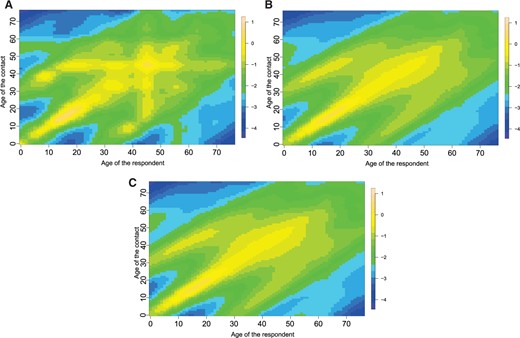
The estimated log contact rates surface, |$\hat{\mathbf{H}}$|, for models |$\mathcal{M}_0$| (A), |$\mathcal{M}_1$| (B) without kink, and |$\mathcal{M}_2$| without kink (C) with the NB1 distribution.
The estimated social contact rates are very similar for models |$\mathcal{M}_1$| and |$\mathcal{M}_2$| (see Figure 4 and Figure 3 of the supplementary material available at Biostatistics online). Further, based on the conclusions of the simulation study and the fact that |$\mathcal{M}_2$| is less computationally intensive, we prefer the use of model |$\mathcal{M}_2$| for the POLYMOD Belgian social contact.
In Figure 5, estimated contact surfaces are shown for model |$\mathcal{M}_2$| with kink for NB1 (95|$\%$| confidence intervals provided in Figure 4 of the supplementary material available at Biostatistics online). It is observed that the main diagonal has higher values for younger ages for the model including the kink and thus higher values on the main diagonal of |$\hat{\mathbf{H}}$| and |$\hat{\boldsymbol{\Gamma}} \odot \mathbf{P}$|. For the model without kink, the values in the estimated matrix |$\hat{\boldsymbol{\Gamma}} \odot \mathbf{P}$| range from 1496.2 to 162 986.5, whereas for the model with kink, the values range from 1608.4 to 375 371.5. The kink thus allows for a huge increase in the estimated number of contacts for children and young adults with individuals of the same age. These results enforce the fact that a kink can capture the effect of mixing with people of the same age, especially for children and young adults.
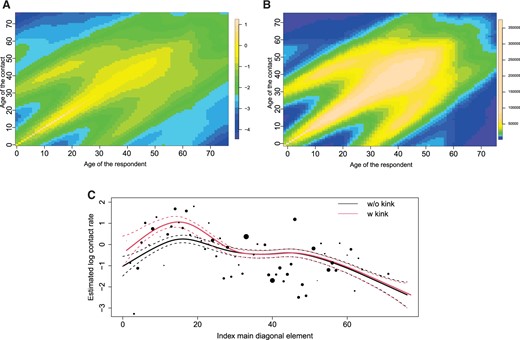
The estimated log contact rates surface (A), |$\hat{\mathbf{H}}$|, and the mixing at the population level (B), |$\hat{\boldsymbol{\Gamma}} \odot \mathbf{P}$|, for model |$\mathcal{M}_2$| with the NB1 distribution including an additional kink on the main diagonal. The diagonal elements of |$\hat{\mathbf{H}}$| for the model with and without a kink (C), together with the |$95\%$| confidence intervals based on 5000 simulation from (2.17). The dots indicate the observed log-contact rates and are proportional to the number of respondents of age |$i-1$|, |$r_{i}$|.
5. Discussion
Quantifying contact behavior contributes to a better understanding of how infectious diseases spread (Anderson and May, 1991; Edmunds and others, 1997). Social contact rates play a major role in mathematical models used to model infectious disease transmission. In this article, we describe a smoothing constrained approach to estimate social contact rates from self-reported social contact data. The proposed approach assumes that the contact rates are smooth from a cohort perspective as well as from the age distribution of contacts by following two alternative strategies.
The simulation study and the data application show that approach |$\mathcal{M}_2$|, in which the penalty matrix is reordered (and penalization is performed over the diagonal components), is performing better. It was observed that this method yielded the smallest MSE over all simulation settings. Additionally, confidence intervals with nominal coverage close to 95|$\%$| were obtained. In the Belgian data application, the computation time of method |$\mathcal{M}_2$| is three to four times faster than method |$\mathcal{M}_1$|, and so we recommend the use of the former approach for the estimation of social contact rates.
The true social contact surface used in the data-generating process of the simulation study was obtained through local linear regression of the raw social contact rates of the Belgian POLYMOD study. This approach is preferred for two reasons. First, by using the same data in the simulation study as in the application presented in Section 4, a better view of the performance of the different approaches can be obtained. Second, we are not aware of any easy applicable mathematical formula or fully parametric model of a 2D surface that would be suitable to represent a contact rate surface.
A grid search is needed to calibrate the smoothing parameters |$\lambda_{1}$| and |$\lambda_{2}$|. This is a disadvantage compared to the approach by van de Kassteele and others (2017) in which the amount of smoothing is directly estimated together with model parameters from the information in the data. However, with the availability of fast parallel computing and multicore machines, the grid search can be performed relatively fast.
In this article, the contact rates are assumed indifferent for men and women. Recently, van de Kassteele and others (2017) presented a Bayesian model for estimating social contact rates for men and women, with results suggesting that different contact patterns exist and thus that there is a gender effect. Future work could investigate how the methodology proposed in this article can be extended to estimate social contact rates by subgroups. A comparison with other methods used to smooth social contact data was not done in this article.
Future extensions could focus on the impact of social contact matrices obtained from different methods on key epidemiological parameters. In general, age-specific contact rates are also used as an input in the comparison and evaluation of vaccination schedules via future projections (Beutels and others, 2013). Most evaluations assume a fixed social contact rate matrix and thus no uncertainty is related to this input. The result derived in (2.17) offers a tool to account for the variability associated with the estimation of social contact rates. By simulation of new contact matrices from (2.17), the associated variability can be taken into account in the evaluation of vaccination strategies and related health economic evaluations.
Finally, our proposed methodology does not employ any regression basis such as B-splines because an exact link between the constraints and linear predictors is needed. We are exploring whether the proposed methodology can be extended to make use of basis functions that will likely lead to a reduction of the computational cost. Alternative ways of incorporating the reciprocal nature of the phenomenon will thus be necessary.
To ensure enough flexibility, no ad hoc choices about the age categories are made in modeling the contact matrices. Additionally, more and more mathematical models of infectious disease transmission use the high-dimensional 1-year matrices. The model-based approach as introduced here can deal with sparsity for certain cells in the matrix (i.e., cells for which few data/information is available). Nevertheless, if an age-stratified modeling approach is of interest, one can choose to directly estimate the contact rates in the different age groups taking the constraint of reciprocity into account (see Hens and Wallinga, 2019) or use our proposed diagonal smoothing approach on a social contact matrix using age categories (see Mossong and others (2008) for an example without diagonal smoothing). Alternatively, the smooth contact surface obtained from diagonal smoothing can still be used to come up with estimates for each combination of age categories by collapsing cells, however, this would surpass the goal of the proposed approach. Our method can be used for extrapolation to provide estimates of contact rates outside the age range observed in the data. However, we warn against doing this, as a more recent study for Belgium (anno 2010–2011) as opposed to the data used here (anno 2006) looked at contact data for individuals up to 99 years of age, and has shown that care needs to be taken when doing so given that contact rates still change substantially for older age groups (Van Hoang and others, 2021).
6. Software
Code to reproduce the results of this article is available at the GitHub repository https://github.com/oswaldogressani/Cohort_smoothing.
Supplementary material
Supplementary material is available online at http://biostatistics.oxfordjournals.org.
Acknowledgments
For the simulation study with the negative binomial model, we used the infrastructure of the VSC Flemish Supercomputer Center, funded by FWO and the Flemish Government—department EWI. Support from the University of Antwerp scientific chair in Evidence-Based Vaccinology is acknowledged to N.H.
Conflict of Interest: None declared.
Funding
This project has received funding from the European Research Council (ERC) under the European Union’s Horizon 2020 research and innovation programme (grant agreement 682540 - TransMID). The European Union’s Research and Innovation Action EpiPose (101003688 to O.G., N.H., and C.F.).
References
Eurostat. (
