


Summary
Whole-brain connectome data characterize the connections among distributed neural populations as a set of edges in a large network, and neuroscience research aims to systematically investigate associations between brain connectome and clinical or experimental conditions as covariates. A covariate is often related to a number of edges connecting multiple brain areas in an organized structure. However, in practice, neither the covariate-related edges nor the structure is known. Therefore, the understanding of underlying neural mechanisms relies on statistical methods that are capable of simultaneously identifying covariate-related connections and recognizing their network topological structures. The task can be challenging because of false-positive noise and almost infinite possibilities of edges combining into subnetworks. To address these challenges, we propose a new statistical approach to handle multivariate edge variables as outcomes and output covariate-related subnetworks. We first study the graph properties of covariate-related subnetworks from a graph and combinatorics perspective and accordingly bridge the inference for individual connectome edges and covariate-related subnetworks. Next, we develop efficient algorithms to exact covariate-related subnetworks from the whole-brain connectome data with an |$\ell_0$| norm penalty. We validate the proposed methods based on an extensive simulation study, and we benchmark our performance against existing methods. Using our proposed method, we analyze two separate resting-state functional magnetic resonance imaging data sets for schizophrenia research and obtain highly replicable disease-related subnetworks.
1. Introduction
Brain connectome analysis has attracted growing research interest in the field of neuroscience, aiming at revealing systematic neurophysiological patterns associated with human behaviors, cognition, and brain diseases (Simpson and others, 2013; Hu and others, 2022). In the past two decades, developments in neuroimaging techniques—including functional magnetic resonance imaging (fMRI) and diffusion tensor imaging—have facilitated large-scale measurements of whole-brain functional and structural connectivity (Bowman and others, 2012). In these experiments, brain neuroimaging data are collected for each participant to form a brain connectivity network characterizing the wiring among neural populations.
The brain connectome data can be encoded as a set of weighted networks on a common set of nodes shared by all participants, where a node represents a brain area and a weighted edge delineates the strength of the functional covariation or structural linkage between brain areas (Lukemire and others, 2021; Xia and Li, 2017; Cai and others, 2019; Warnick and others, 2018). Participants with different behavioral and clinical conditions tend to exhibit distinct brain connectivity patterns at global and local levels. In these studies, statistical methods have played a central role in discovering the systematic effects of a covariate (e.g., a clinical condition) on brain networks and have led to a comprehensive understanding of the underlying neurophysiopathological mechanisms (Zhang and others, 2017; Durante and others, 2018; Kundu and others, 2018; Cao and others, 2019; Wang and others, 2019).
In the present research, we focus on statistical methods for modeling multivariate connectivity edges constrained in a connectome adjacency matrix as outcomes and clinical and demographic conditions as covariates (Simpson and others, 2019; Zhang and others, 2023). These methods are alternatives to covariate-related connectivity network methods using principal component analysis and independent component analysis techniques (e.g., Shi and Guo, 2016; Zhao and others, 2021) that take time series at multiple brain regions as the input connectome data for each participant. Therefore, the two sets of methods can provide complementary perspectives to characterize the connectome patterns associated with the covariate of interest. In the neuroimaging literature, brain network analysis often refers to the analysis of prespecified “networks” (e.g., default mode network [DMN]), which boils down to assessing the association between the covariate and the averaged connection strength of edges in the network (Craddock and others, 2013). However, analysis of prespecified networks may miss the true covariate-related network while introducing false-positive findings. Lastly, cluster-wise multivariate edge inference methods (e.g., network-based statistic [NBS]) have also been used widely with the control of family-wise error rate (FWER) (Zalesky and others, 2010). The covariate-related networks in NBS are formed by a three-step procedure: (i) performing statistical analysis on each edge and attaining corresponding test statistics; (ii) applying a threshold to the test statistics of all edges and then searching the maximally connected networks of suprathreshold edges in the whole-brain connectome; (iii) conducting permutation tests for detected networks to control FWER. However, based on graph theories, a small proportion of suprathreshold covariate-related edges based on a sound threshold can almost surely connect all nodes in the connectome (Stepanov, 1970), and selecting subnetworks as a set of covariate-related edges involving all brain areas is less biologically meaningful (Craddock and others, 2013). Consequently, utilizing current methods for covariate-related network analysis (e.g., NBS) can result in a subpar inferential accuracy due to the presence of false-positive noise that hinders the extraction of subnetworks and the lack of statistical theory for testing extracted subnetworks.
To fill this gap, we propose a procedure called Statistical Inference for Covariate-Related Subnetworks (SICERS). We first define a covariate-related subnetwork as a set of edges associated with the covariate of interest that constitute an organized graph structure (e.g., a community and interconnected communities). Evaluating the network-level effect of a covariate on the whole-brain connectome requires (i) identifying subnetworks concentrated with covariate-related edges and (ii) allocating a large proportion of covariate-related edges into covariate-related subnetworks. We first show that given no network-level effect of a covariate, the chance of discovering a moderate-sized subnetwork concentrated with covariate-related edges is close to zero (by Lemma 2.1). In other words, detecting a reasonably sized and dense covariate-related subnetwork suggests the true effect on a brain network. This property is critical and motivates our method developments for subnetwork extraction and network-level inference. We demonstrate the SICERS procedure in Figure 1.
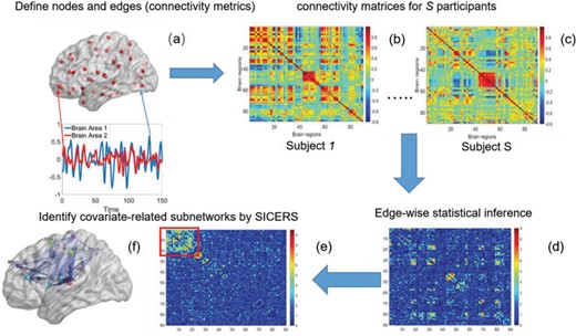
The SICERS pipeline: (a) define brain regions as nodes and connectivity metrics between each pair of nodes as edges; (b) and (c) calculate the connectivity matrix for each single subject in a study, where each off-diagonal element in the matrix represents the connectivity strength between two nodes, then identify differential connectivity patterns between clinical groups; (d) plot the edge-wise statistical inference, where each off-diagonal element is a negatively logarithmically transformed |$p$|-value (e.g., two-sample-test |$p$|-value per edge between clinical groups and a hotter point in the heatmap suggests larger group-wise difference); (e) reveal the disease-related subnetwork detected by SICERS; (f) show the corresponding 3D (3D) brain image. Note that (e) was obtained by reordering the nodes in (d) by listing the detected subnetwork first (i.e., these two graphs are isomorphic).
The article makes several contributions. First, our method provides a new tool for handling multivariate edge variables in brain connectome data for covariate-related subnetwork analysis. We develop a strategy to consolidate edge- and network-level analysis from a graph and combinatorics perspective, and propose an inference approach that is designed to test data-driven subnetworks (i.e., not prespecified) using a graph probabilistic model. Second, we develop an efficient algorithm to optimize the objective function for covariate-related subnetwork detection, which integrates dense subgraph extraction and community detection by imposing an |$\ell_0$| penalty on network edges. The |$\ell_0$| shrinkage term can effectively reduce the impact of false-positive noise and thus minimizes false-positive subnetwork detection. Our algorithm is also compatible with computationally intensive inference methods (e.g., permutation tests). Lastly, our findings in the data example reveal a novel schizophrenia-disrupted brain connectivity network that links three primary disease-related subnetworks including the DMN, salience network (SN), and central executive network (CEN) (Manoliu and others, 2014).
2. Methods
2.1. Background: brain connectome data and edge-wise inference
We denote |$\boldsymbol{Y}_{n\times T}^s$| as the region-level fMRI time series for a participant |$s=1, \ldots, S$|, where |$n$| is the number of regions of interest, and |$T$| is the length of time series. We assume that fMRI data are registered into a common template and thus brain regions are identical across participants (e.g., the Brainnetome Atlas by Fan and others, 2016). Let |$a^s_{ij}$| denote the connection strength between a pair of regions |$1 \leq i<j \leq n$|, which can be calculated by the correlation (or partial correlation/spectral coherence) between the two corresponding region-wise time series. A weighted |$n \times n$| adjacency matrix |$\boldsymbol{A}^s=\{a^s_{ij}\}$| records all |$n(n-1)/2$| pair-wise connectivity measures for participant |$s$|. |$\boldsymbol{A}^s\}$| maps to a population-level brain connectome structural graph |$G=\{V, E\}$|, where the node set |$V$| (|$|V|=n$|) represents regions of interest, the edge set |$E=\{e_{ij}\}$| indicates the functional connections between regions. |$V$| and |$E$| are identical across participants because we assume that the neurobiological definitions of brain regions and connectivity are shared across participants (Simpson and others, 2013). |$\boldsymbol{A}^s$| are multivariate random variables capturing the connection strengths of an individual, and thus outcomes. In addition, for each participant, we observe a vector of profiling covariates (e.g., the clinical status and demographic variables), denoted by |$\boldsymbol{x}_s= (x_{s,1}, \ldots, x_{s,L})^T$|.
Our goal is to assess the associations between |$\boldsymbol{A}^s$| and |$\boldsymbol{x}_s$|, revealing the underlying covariate-related neural connectomic mechanisms. Naturally, one can apply commonly used multivariate statistical models (e.g., multiple testing, regularized correction, and low-rank regression models) to identify a set of edges associated with covariates of interest. Consider a generalized linear model (Zhang and others, 2023):
Without loss of generality, we focus on one covariate of interest (e.g., clinical diagnosis) while adjusting for other confounding variables. Because subnetworks can vary among different covariates, we can perform covariate-specific subnetwork analysis and apply the procedure for each covariate of interest or interaction. Let |$\boldsymbol{B} = \{\beta_{ij}\}$| be the associated matrix of regression coefficients of interest. Then, the corresponding edge-wise hypotheses are
As our interest is to identify covariate-related subnetworks instead of individual parameters that |$\beta_{ij} \neq 0$|, we present |$\{ \beta_{ij} \}$| in a binary graph |$G^\beta= \{V, E^\beta\},$| where |$e^\beta_{ij}=1$| if |$\beta_{ij} \neq 0$| otherwise 0. In practice, we note that covariate-related edges |$\{ \beta_{ij} \neq 0 \}$| only contribute a small proportion of edges in the brain connectome (Chen and others, 2016), and more importantly their appearance in the network is concentrated in a few block-structured subnetworks (i.e., |$G^\beta$| is not random). Our proposed SICERS method will provide novel procedures for estimation and inference on these latent covariate-related subnetworks to answer the fundamental scientific problem of how a covariate of interest systematically affects the brain connectome.
2.2. The general model
As a starting point, we propose a general graph model that decomposes the population brain connectome structural graph into subnetworks related to the covariate and a subgraph that is not related to the covariate:
where each |$G_c= \{V_c, E_c\}$| is a covariate-related subnetwork, |$C$| is the number of subnetworks (neural subsystems) altered by the covariate, and |$G_0=\{V_0,E_0 \}$| is the remainder of |$G$| (i.e., covariate irrelevant). Specifically, |$V=\cup_{c=1}^C V_c \cup V_0$| , |$V_c\cap V_{c'}=\emptyset,$| and |$E=\cup_{c=1}^C E_c \cup E_0$|. In other words, |$G$| is formed by the union of |$C$| mutually disjoint covariate-related subnetworks |$G_1,\ldots, G_C$| and singleton nodes that do not belong to any subnetwork. |$G_0$| is defined as a union of singleton nodes and edges not in |$\left(\cup_{c=1}^C G_c\right)$|. |$G_c$| distinguishes itself from |$G_0$| as the density of covariate-related edges is higher in |$G_c$| than |$G_0$|, that is, |$\sum_{i,j \in G_c}I(\beta_{ij} \neq 0) / |E_c| >\sum_{i,j \in G_0}I(\beta_{ij} \neq 0)/(|E|-\sum_{c=1}^C|E_c|)$|. We further define |$\ell_0$| as the graph norm that measures the number of edges of a covariate-related subnetwork of |$G_c$|, that is, |$\|G_c\|_0=|E_c|$|. Consequently, |$\|G_0\|_0=0$| and |$\sum_{c=1}^C |E_c| < n(n-1)/2$| assuming that |$\left(\cup_{c=1}^C G_c\right)$| covers all nonisolated covariate-related edges.
Our model is closely related to but distinct from classical network models. When |$C=0$|, the model can be viewed as an Erdős–Renyi graph. In the general scenarios where |$C>0$|, our model differs from the traditional block structure in clustering and community-detection algorithms because our focus is on covariate-related subnetworks |$\left(\cup_{c=1}^C G_c\right)$| while treating |$G_0$| as irrelevant information. |$G_0$| consists exclusively of singletons and has |$|V_0|=\sum_{i}^n I(i \in G_0)$| and |$\|G_0\|_0=0$|, which resembles the nondense component of the dense subgraph model (Wu and others). On the other hand, our method differs from dense subgraph discovery models because we simultaneously consider multiple subnetworks |$G_1,\ldots, G_C$|. Therefore, our model is a combination of a dense subgraph model and a block structure model.
2.3. Statistical inference for covariate-related subnetworks
The statistical inference for covariate-related subnetworks |$\{G_c\}$| is distinct from the classical statistical inference on a single well-defined parameter (e.g., |$\beta_{ij}$|). In the context of graph models, the inference of |$G_c$| is naturally linked with graph theory and combinatorics. We propose a statistical inference framework to test covariate-related subnetworks when neither |$\{G_c\}$| nor |$C$| is known in (2.3). We consider the following test for the existence of the subnetwork structure:
Here, |$C=0$| means |$\sum_{c=1}^C|E_c|=0$|, that is, no covariate-related subnetwork exists. We propose the following lemma (2.1) as a graph–combinatorics-based procedure, to determine the rejection region for (2.4) based on the graph properties of subnetworks (i.e., the size and density of a subnetwork).
Specifically, we derive lemma (2.1) for network-level inference in the context of association parameter binary graph |$G^{\beta}$| and covariate-related subnetworks defined by the general model of population connectome structural graph |$G=\left(\cup_{c=1}^C G_c\right) \cup G_0$|. Without loss of generality, we define the densities of |$G$| and covariate-related subnetworks subgraph by
Directly developing inference method for covariate-related subnetworks is challenging, because |$\hat{G}_c$| is unknown before analyzing the sample data. We adopt the concept of “maximum quasiclique” in graph theory as an alternative to develop the inference theory while alleviating the required prior knowledge of |$G_c$|. In |$G^{\beta}$|, for any |$\gamma\in(p,1)$|, we call a subnetwork of this binary network a “|$\gamma$|-quasi clique” if its observed edge density is at least |$\gamma$|. Define a maximum |$\gamma$| quasiclique |$G^{\beta}[\gamma]$| to be the largest-in-size |$\gamma$|-quasi clique in |$G^{\beta}$|, and let |$|G^{\beta}[\gamma]|$| be the number of nodes in |$G^{\beta}[\gamma]$|. |$G^{\beta}[\gamma]$| can be detected using computationally efficient procedures in the existing literature; see Wu and Hao (2015) for a comprehensive review. Under the null hypothesis |$H_{G;0}$|, the graph |$G^{\beta}$| becomes an Erdős–Renyi graph with |$p=q$|. Next, we derive the probability bounds for the size given density for |$G^{\beta}[\gamma]$| under |$H_{G;0}$| and |$H_{G;1}$|.
In a binary graph |$G^{\beta}$|,
- when |$H_{G;0}: C\,{=}\,0$| is true, that is, |$p\,{=}\,q$|, assume that for any |$\gamma\in(p,1)$|, |$v_0\,{=}\,\omega(\sqrt{n})$| where |$\omega$| denotes a loose lower bound, and |$n$| large enough such that |$\{ 4/(\gamma-p)^2+ 4/[3(\gamma-p)]\}^{-1} v_0\geq \log n$|. Then, we have$$ {\mathbb{P}}\left( |G^{\beta}[\gamma]|\geq v_0|H_{G;0} \right) \leq 2n\cdot \exp\left( -\left\{\frac{4}{ (\gamma-p)^2} +\frac{4}{3(\gamma-p)} \right\}^{-1}\cdot v_0^2 \right)\!.$$
- when |$H_{G;a}: C\geq 1$| is true, assume that all subnetworks satisfy |$|G_c| >\omega(\sqrt{n})$| and set |$v_0=c_0\sqrt{n}$| for a small enough constant |$c_0>0$|, such that |$\min_{c=1,\ldots,C} |G_c|\geq v_0$|. Then, we have$$ {\mathbb{P}}\left( |G^{\beta}[\gamma]| \geq v_0 |H_{G;a} \right) \geq 1-\exp\left\{ -\frac{(q-\gamma)^2 v_0(v_0-1)/4}{1+(q-\gamma)/3} \right\}\!.$$
Intuitively, Lemma 2.1 states that (i) the probability of a nonsmall and dense subnetwork existing under |$H_{G;0}$| is almost zero, whereas (ii) the probability of a nonsmall and dense subnetwork existing under |$H_{G;1}$| approaches 1. Therefore, the probability bounds in Lemma 2.1 can be used to calculate both the type I error rate of an observed |$\hat{G}_c$| and the strength of |$\hat{G}_c$| associated with the covariate. Under simple scenarios where there is only one subnetwork present in |$G$|, we can directly calculate the type I error of |$\hat{G}_c$| by |$2n\cdot \exp\left( -\left\{\frac{4}{ (\gamma-p)^2} +\frac{4}{3(\gamma-p)} \right\}^{-1}\cdot|\hat{G}_c|^2 \right)$|, and then reject |$H_{G;0}$| if the type I error is less than the significance level |$\alpha$|. However, the inference procedure in our application is more complex as multiple covariate-related subnetworks may exist. In the field of neuroimaging statistics, a widely used statistical inference method for simultaneously testing multiple covariate-related subnetworks |$\hat{G}_1,\ldots,\hat{G}_C$| is the family-wise error control (FWER) strategy (e.g., permutation tests), which requires comparing subnetworks with different densities and sizes. For example, |$G_c$| and |$G_c'$| are subnetworks with densities and sizes (|$\gamma$|, |$v_0$|) and (|$\gamma'$|, |$v_0'$|) respectively. Lemma 2.1 provides a viable solution for the comparison by calculating two probability bounds |$2n\cdot \exp\left( -\left\{\frac{4}{ (\gamma-p)^2} +\frac{4}{3(\gamma-p)} \right\}^{-1}\cdot v_0^2 \right)$| versus |$2n\cdot \exp\left( -\left\{\frac{4}{ (\gamma'-p)^2} +\frac{4}{3(\gamma'-p)} \right\}^{-1}\cdot v_0'^2 \right)$|. The subnetwork with a lower probability bound is considered to have a stronger association with the covariate, as it is less likely to occur under |$H_{G;0}$| (see details in Section 2.5).
2.4. Extracting covariate-related subnetworks via ℓ0 graph norm penalty
We aim to extract covariate-related subnetworks |$\{G_c\}$| from the dependent variables and covariates |$\{\boldsymbol{A}^s, \boldsymbol{x}_s\}_{s=1}^S$|. We first estimate and test |$\{\beta_{ij}\}$| by (2.1). For a continuous brain connectivity measure (e.g., Fisher’s Z transformed correlation coefficients), both classic general linear model and autoregressive multivariate model accounting for the dependence can be applied (Bowman, 2005; Chen and others, 2020). Although the latter provides a more accurate inference (particularly for a small sample), the computational cost is much higher. In practice, for a sample of hundreds of participants, we adopt the general linear model because the statistical inference results of these two methods show little difference. The statistical inferential results for |$\{\beta_{ij}\}$| (e.g., the test statistics or |$p$|-values) can be stored in a matrix |$\boldsymbol{W}=\{w_{ij}\}$| (e.g., |$w_{ij} = -\log(p_{ij})$|), which will be used as the input to extract covariate-related subnetworks. We adopt |$p$|-values (and |$-\log(p_{ij})$|) due to its popularity in high-dimensional data analysis [e.g., false-discovery rate (FDR) and Manhattan plot] and capability to discern |$\beta_{ij} \neq 0$| versus |$\beta_{ij}= 0$|. Nevertheless, our method is applicable to |$\boldsymbol{W}$| generated from any valid statistical model.
Our goal is to cover covariate-related edges using a set of well-organized subgraphs with minimal (edge) sizes to achieve inference efficiency and accuracy in accordance with Lemma 2.1. We constrain subnetworks |$\{G_c\}$| in a plausible network structure, where |$G=\left(\cup_{c=1}^C G_c\right) \cup G_0$|, for the reasons stated in Section 2.2. Therefore, our model resembles but is distinct from the stochastic block model, where all nodes are assigned to a few communities, and the submatrix model, which only covers |$C=1$|. This graph structure—with several small communities and a majority of singleton nodes—poses a unique challenge for estimation. This is determined by the fact that a small proportion of edges are associated with the covariate.
As a highlight of our method, while most conventional community-detection techniques for stochastic block models typically demand relatively balanced community sizes |$|V_1|, \ldots,|V_c|$| that would contain most nodes |$|V_1|+\cdots+|V_C|=n$| or |$\approx n$|, our method addresses the case where all the blocks |$|V_c|$| put together could constitute only a small portion of the whole graph, that is, |$\sum_{c=1}^C |V_c|\ll n$|. Therefore, our approach can be considered as a tool for informative subnetwork extraction rather than clustering or community detection. As illustrated in Figure 2, several conventional community-detection techniques may encounter difficulties in extracting meaningful subnetworks from the inference matrix |$\boldsymbol{W}$| of an rs-fMRI brain connectome study (Adhikari and others, 2019).
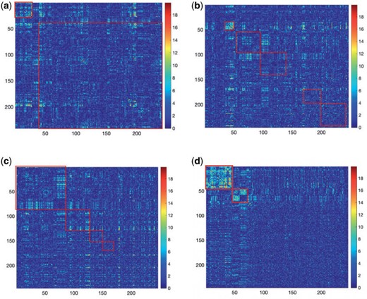
Subnetwork extraction by SICERS versus classical community-detection algorithms on a |$\boldsymbol{W}$| matrix with a structure of |$G=\left(\cup_{c=1}^C G_c\right) \cup G_0$|: (a) spectral clustering with 10 communities in Von Luxburg (2007); (b) Louvain method by Blondel and others (2008); (c) INFOMAP algorithm by Rosvall and Bergstrom (2008); (d) SICERS community detection.
To extract covariate-related subnetworks based on |$\boldsymbol{W}$| appears a conceptually straightforward approach by optimizing a valid objective function (e.g., likelihood function) in the conventional network community-detection literature (Bickel and Chen, 2009; Zhao and others, 2012). However, the results of these methods tend to yield subnetworks with a small proportion of covariate-related edges due to the false-positive noise. Instead, we resort to an |$\ell_0$| graph norm penalty-based objective function to extract covariate-related subnetworks from |$\boldsymbol{W}$|, where most edges are associated with the covariate. Our objective function is inspired by Lemma 2.1 and is thus specifically tailored for subnetwork-wise inference. The idea is very simple: for any detected subnetwork |$\hat{G}_c$|, we reward edge weights within this subnetwork while penalizing based on its size (i.e., increasing density and size). This objective function can lead to the discovery of a set of subnetworks with the maximal density and number of covariate-related edges. As shown in Lemma 2.1, the probability of observing a certain-sized covariate-related subnetwork (a |$\gamma$|-quasi clique) is slim with a high density |$\gamma$|. Similar ideas have been adopted in some network community-detection methods (Zhang and others, 2016). Specifically, we define
where “|$*$|” denotes the Hadamard (element-wise) matrix product and |$\delta_{ij}=1$| if |$i,j \in \forall G_c$| and 0 otherwise. Clearly, |$\bf{U}$| depends on the specified structure of the underlying graph |$G=(\delta_{ij})_{i,j}$|. Define |$\|\textbf U\|_1 = \sum_{i,j}|u_{ij}|$| and |$\|\textbf U\|_0=\sum_{i,j}I(|u_{ij}|>0)$|, where |$\|\quad\|_1$| and |$\|\quad\|_0$| are matrix-element-wise |$\ell_1$| and |$\ell_0$| norms. |$\|\textbf U\|_0$| is equivalent to the |$\ell_0$| graph norm, because we define |$\|G\|_0 =\sum_c^C \sum_{e_{ij}\in G_c} I(\delta_{ij}=1)$| in Section 2.2. Our core proposal is the following |$\ell_0$| graph norm shrinkage criterion:
where |$\lambda_0$| is a tuning parameter.
Optimizing the objective function (2.7) simultaneously estimates the number of subnetworks and the subnetwork memberships of all nodes in |$G = \cup_{c=1}^C G_c \cup G_0$|. Here, we consider a singleton as a subnetwork. The objective function (2.7) maximizes the edge weights with minimally sized subnetworks, which is mathematically equivalent to extracting maximally sized subnetworks (quasicliques) sizes while maximizing the density. Therefore, the optimization of (2.7) is governed by two goals: covering high-weight informative edges and using minimally sized subnetworks. Maximizing the first term |$\|\bf{U}\|_1$| can increase sensitivity by allocating a maximal number of high-weight edges to subnetworks, which promotes larger subnetworks; this is concordant with our aforementioned views in Section 2.3. In that, prespecifying density |$\gamma$| in Lemma (2.1) is not required because 2.7 automatically maximizes subnetwork density and size. We also penalize the |$\ell_0$| graph norm for maximizing the density of subnetworks. The second term can also suppress false-positive noise, because false-positive edges tend to be distributed in a random pattern in |$G$| rather than in an organized subgraph (Chen and others, 2015).
The conflicting nature of the two goals leads to a balance between the different goals that they represent in the optimization procedure, thereby producing meaningful results. The balance between them is tuned by |$\lambda_0$|; specifically, |$\lambda_0=0$| would send all nodes to one subnetwork, whereas a large |$\lambda_0$| prefers small communities and singletons (nodes not in any community, thus contributing zero |$\ell_0$| graph norm) even to the true community structure. In our theoretical analysis, we specify the range of tuning parameter |$\lambda_0$| (depending on |$\mu_0/\mu_1$|) in which our criterion provides a consistent estimation of the community structure, thereby controlling well the rates of both types of errors in the multiple testing procedure. In practice, select |$\lambda_0$| based on the likelihood function of the network (see supplementary material available at Biostatistics online).
We optimize (2.7) and extract covariate-related subnetworks using Algorithm 1. Specifically, we perform a grid search for |$C$|. For each value of |$C=C^\dagger$|, let |$\hat{G}(C^\dagger)$| be the estimated network structure by optimizing (2.7), and let |$\textbf{U}_{\hat{G}(C^\dagger)}$| be the corresponding matrix from Hadamard matrix multiplication. |$\textbf{U}_c$| is the submatrix of |$\textbf{U}$| corresponding to |$G_c$|. The outcome provides a set of maximal subnetworks with high density. In the supplementary material available at Biostatistics online, we provide detailed implementation and theoretical results to guarantee the consistency and optimality of |$\hat{C}, (\hat{G}_c)_{c=1,\ldots,\hat{C}}$|.
Subnetwork estimation
Data: Input: |$\boldsymbol{W}$|; tuning parameter |$\lambda_0$|
1. For |$C ^\dagger= 2$| to |$n-1$|
2. Optimize |$\mathop {\arg \,\max } \limits_{ G(C^\dagger)} \sum_{c=1}^{C^\dagger} \frac{\|\textbf{U}_c \|_1}{\|\textbf{U}_c \|_0^{\lambda_0}}$| (see details in the supplementary material available at Biostatistics online)
3. Select |$\hat{C}$| such that |$\mathop {\arg \,\max } \limits_{C^\dagger=2, \ldots, n-1} \log \| { \textbf{U}_{\hat{G}(C ^\dagger) }} \|_1 -\lambda_0 \log \| {\textbf{U}_{\hat{G}(C ^\dagger)}}\|_0$|
Output:|$\hat{C}, (\hat{G}_c)_{c=1,\ldots,\hat{C}}$|
2.5. Testing covariate-related subnetworks
Given a set of estimated covariate-related subnetworks |$(\hat{G}_c)_{c=1,\ldots,\hat{C}}$|, our goal is to assess statistical significance for each subnetwork. This is more general than the aforementioned hypothesis test (2.4) because the subnetwork-wise inference is needed for more than one subnetwork. Note that the testing hypothesis on a covariate-related subnetwork |$\hat{G}_c$| is distinct from classical statistical hypothesis tests because the parameters of the null hypothesis are based on an estimated |$\hat{G}_c$| rather than prespecified parameters. Because a subnetwork |$\hat{G}_c$| can be considered as a cluster of edges, we adopt the commonly used permutation tests to examine the significance of |$\hat{G}_c$| while controlling FWER (Zalesky and others, 2010; Nichols, 2012; Chen and others, 2015). However, the test statistic in the classic permutation tests is often trivial (e.g., using the number of supra-threshold edges in |$\hat{G}_c$| as the test statistic). Building on Lemma 2.1, we propose a new test statistic to reflect the combinatorial probability for a covariate-related subnetwork with a given density and size under the null hypothesis. We present the steps of our test in Algorithm 2.
Assess the significance of |$\hat{G}_c$|
Data: Input: |$\{\boldsymbol{A}^s, \boldsymbol{x}_s \}_{s=1,\ldots, S}$|, |$W$|, |$\hat C>0$|, |$\{\hat G_c\}_{c=1,\ldots,\hat C}$|, |$g(r)$|, |$\alpha$|
1. With a sound cut-off |$\hat{r}$|, set the binarized graph |$G[\hat{r}]: (G[\hat{r}])_{ij}=I(w_{ij}>\hat{r})$|
2. Estimate overall and within-subnetwork edge densities |$\hat p$| and |$\hat q$|
and set |$\hat\gamma:= \hat{q}$|
3. Calculate (Lemma 2.1) |$p$|-value-based test statistic by integrating |$r$| on its distribution |$g(r)$|: |$\mathcal{T}_0 ( \hat G_c )=\int 2n\cdot \exp\left\{ -|\hat{G}_c|^2\left\{\frac{2}{ (\hat\gamma-\hat{p})^2} +\frac{2}{3(\hat\gamma-\hat{p})} \right\}^{-1} \right\}g(r) {\rm d}r$|
4. Shuffle the group labels of the data and implement SICERS |$M$| times, and for each simulation |$m=1, \ldots, M$|, store the maximal test statistic |$\mathcal{T}_m=\sup_{c=1,\ldots,\hat C^m} \int 2n\cdot \exp\left\{ -|\hat{G}^m_c|^2/\left\{\frac{2}{ (\hat\gamma_m-\hat{p}_m)^2} +\frac{2}{3(\hat\gamma_m-\hat{p}_m)} \right\}^{-1} \right\}g(r){\rm d}r$|
5. Calculate the percentile of |$\mathcal{T}_0$| in |$\{\mathcal{T}_m \}$| as the FWER |$q$|-value and reject the null hypothesis if |$q<\alpha$|
Output: FWER significance values for |$\{\hat G_c\}_{c=1,\ldots,\hat C}$|
The above procedure can also be used to test the omnibus hypothesis (2.4) for |$C=0$| versus |$C>0$|, because any single reasonably sized and dense subnetwork |$\hat{G}_c$| can lead to a small |$p$|-value. The null distribution of the test statistic in (2.4) can be simulated well by the permutation procedure. Therefore, the FWER can be controlled effectively by the above permutation test, yielding a corrected |$p$|-value for each |$\hat{G}_c$| (Nichols, 2012).
3. Simulations
In this section, we evaluate the performance of our method on synthetic data and compare it with benchmarks. We assess the accuracy of SICERS on two levels: (i) subnetwork-level inference accuracy by tallying the false-positive and false-negative covariate-related subnetworks; (ii) edge-level assessment to measure the quality of significant covariate-related subnetwork and overall performance by comparing |$\hat{G}_c$| with |$G_c$| and counting the false-positive and false-negative edges. The covariate-related subnetwork inference is satisfactory only if network- and edge-level inference are both accurate.
First, we simulate brain connectome data |$\mathcal{A} = \{\boldsymbol{A}^1,...,\boldsymbol{A}^S\}$| in a common two-sample testing setting, although we can easily extend it to the regression setting. We consider two cohorts of participants with equal sample sizes. We denote healthy controls by |$s=1,\ldots,[S/2]$| and patients by |$s=[S/2]+1,\ldots,S$|, where |$[\;]$| denotes the floor operator. The number of brain regions is |$|V|=n=200$|, and there are 19 000 edges correspondingly. We consider two disease-related subnetworks |$G_1$| and |$G_2$| with |$|V_1|=25$| and |$|V_2|=50$|. For a patient |$s\geq [S/2]+1$|, for all |$(i,j): i\in V_1/V_2, j\in V_1/V_2$|, we set |$a_{ij}^s \sim N(\eta_2, \sigma^2)$|; for all other |$(s,i,j)$|, we set |$a_{ij}^s \sim N(\eta_1, \sigma^2)$|. We vary |$\theta=\eta_2-\eta_1$| and |$\sigma$| to emulate different effect sizes (i.e., signal-to-noise ratios). We set the variance term |$\sigma = 0.5, 1, 2$| given |$\theta=1$|, corresponding to values of Cohen’s |$d$| of |$1.2, 0.8$|, and 0.5, respectively. Two sample sizes of |$S=480$| and |$S=240$| were used. For each combination of parameters, we simulate 100 repeated data sets.
For each brain connectome data set |$\mathcal{A}$|, we perform edge-wise two-sample tests on |$\{a^1_{ij},\ldots, a^{[S/2]}_{ij}\}$| versus |$\{a^{[S/2]+1}_{ij},\ldots, a^S_{ij}\}$| and obtain the inference matrix |$\boldsymbol W$| by |$w_{ij} = -\log p_{ij}$|. We then apply SICERS to |$\boldsymbol W$|, estimating disease-related subnetworks and performing subnetwork-level statistical inference. We benchmark our approach against the popular methods for brain connectivity analysis including NBS and comparable subnetwork extraction methods by dense subgraph extraction algorithms (e.g., greedy) and community-detection algorithms (e.g., Louvain).
Subnetwork-level inference results. First, we evaluate the accuracy of SICERS at the network-level. Correctly identifying a covariate-related subnetwork involves two aspects: (i) extracting a |$\hat{G}_c$| that is close to |$G_c$| and (ii) rejecting the null hypothesis for |$\hat{G}_c$|. Therefore, we consider that our goal of network-level inference is met if SICERS rejects the null hypothesis for an estimated subnetwork |$\hat{G}_c$| that is similar to |$G_c$| (e.g., the Jaccard index for edge sets of |$\hat{G}_c$| and |$G_c$| is greater than 50|$\%$|). We denote an estimated subnetwork as a false-positive finding when we reject the null hypothesis and the Jaccard index between |$\hat{G}_c$| and |$G_c$| is less than 50|$\%$|. We record a false-negative finding for |$G_c$| if we fail to estimate |$\hat{G}_c$| with a Jaccard index of greater than |$50\%$| in reference to |$G_c$| and reject the null hypothesis. We calculate the power and false-positive rate (FPR) as the proportions of true-positive and false-positive inference across the 100 repeated data sets with the corresponding standard errors.
The results for the network-level summarized statistics are presented in Table 1. Our network-level inference is generally robust and accurate for both |$G_1$| and |$G_2$|. The power and FPR of network-level inference rely on the capability of subnetwork extraction because the power is 0 if no |$\hat{G}_c$| is detected and FPR is high if the significant |$\hat{G}_c$| largely deviates from |$G_c$|. The subnetwork extracted by NBS is often different from |$G_c$| due to the influence of noise, which leads to low power and high FPR. The inference accuracy is also determined by the subnetwork size, effect size, sample size, and noise level (results for a range of network sizes are in supplementary material available at Biostatistics online). SICERS outperforms the comparable methods due to the superior performance of its |$\ell_0$| shrinkage-based subnetwork extraction and advanced inference approach (see Algorithm 2).
Network-level inference results across all settings. The power is calculated separately for each of the two subnetworks (|$G_1$||$|V_1|=25$| and |$G_2$||$|V_2|=50$|), while the FPR is based on the aggregate false-positive findings. The means (standard deviations) of power and FPR are summarized based on 100 repeated simulations. SICERS generally performs well for all settings, followed by Louvain, Dense, and NBS. The Power and FPR largely rely on accurate subnetwork extraction and inference. Large subnetwork size, effect size, and sample size can improve the accuracy of subnetwork extraction and yield greater test statistics, thus increase power and sensitivity. SICERS outperforms the other methods because the |$\ell_0$| shrinkage and our new statistical inference methods can better capture and characterize covariate-related subnetworks
| |$S = 240$| | |$S = 120$| | |||||||
|---|---|---|---|---|---|---|---|---|
| Cohen’s |$d$| | 1.2 | 0.8 | 0.5 | 1.2 | 0.8 | 0.5 | ||
| SICERS | Power | |$G_1$| | 1(0) | 0.98(0.14) | 0.84(0.37) | 1(0) | 1(0) | 0.86(0.35) |
| |$G_2$| | 1(0) | 1(0) | 1(0) | 1(0) | 1(0) | 1(0) | ||
| FPR | 0(0) | 0.05(0.13) | 0.03(0.09) | 0(0) | 0.03(0.09) | 0.03(0.09) | ||
| Louvain | Power | |$G_1$| | 1(0) | 0.92(0.27) | 1(0) | 1(0) | 0.86(0.35) | 1(0) |
| |$G_2$| | 1(0) | 1(0) | 1(0) | 1(0) | 1(0) | 1(0) | ||
| FPR | 0.08(0.17) | 0.07(0.16) | 0(0) | 0.11(0.2) | 0.09(0.19) | 0.01(0.05) | ||
| Dense | Power | |$G_1$| | 1(0) | 1(0) | 0.36(0.48) | 1(0) | 1(0) | 0.06(0.24) |
| |$G_2$| | 1(0) | 1(0) | 1(0) | 1(0) | 1(0) | 1(0) | ||
| FPR | 0(0) | 0.33(0) | 0.44(0.08) | 0(0) | 0.33(0) | 0.49(0.04) | ||
| NBS | Power | |$G_1$| | 0.14(0.35) | 0(0) | 0(0) | 0.26(0.44) | 0(0) | 0(0) |
| |$G_2$| | 1(0) | 0(0) | 0(0) | 1(0) | 0(0) | 0(0) | ||
| FPR | 0.1(0.21) | 1(0) | 1(0) | 0.08(0.2) | 1(0) | 1(0) | ||
Edge-level inference results. Given significant covariate-related subnetworks, we further evaluate the deviation of |$\hat{G}_c$| from |$G_c$| by measuring the edge-level difference. The |$\hat{G}_c$| versus |$G_c$| differences are measured at the edge-level with respect to sensitivity and FDR as follows: |$\text{Sensitivity} = \frac{\sum_{i<j}I(e_{ij}\in G_c,e_{ij}\in \hat G_c)}{\sum_{i<j}I(e_{ij}\in G_c)} \text{ and FDR} = \frac{\sum_{i<j}I(e_{ij}\notin G_c,e_{ij}\in \hat G_c)}{\sum_{i<j}I(e_{ij}\in \hat G_c)}.$|
Table 2 summarizes the performance of all methods in all settings. In general, SICERS, network detection, and dense algorithms can recover the covariate-related subnetworks. When the effect size is smaller, network detection and subgraph extraction algorithms tend to cover a maximal number of informative edges and thus also include false-positive edges in the estimated subnetworks; therefore, the detected subnetworks may differ from the true network. SICERS is more robust to false-positive noise for small effect size because it imposes an |$\ell_0$| penalty term on the objective function. NBS is more sensitive to noise because the subnetwork detection extraction algorithm of NBS seeks maximally connected components. Lastly, we compare the network analysis method with the univariate method BH-FDR (|$q=0.05$|). Without the aid of graph information, the univariate inference method tends to select a high proportion of false-positive edges and fails to recognize the network structure.
Edge-level inference results across all settings. The TPR and FDR are calculated separately for each of the two subnetworks (|$G_1$||$|V_1|=25$| and |$G_2$||$|V_2|=50$|). The means (standard deviations) of TPR and FDR are summarized based on 100 repeated simulations. TPR is determined by the proportion of edges in |$G_c$| that can be recovered by |$\hat{G}_c$|, and FDR is the proportion of edges in |$\hat{G}_c$| are not in |$G_c$|. TPR = 1 and FDR = 0 suggest a perfect recovery of |$G_c$| by |$\hat{G}_c$|. SICERS outperforms the comparable methods because the objective function can maximize the signal while suppressing noise, and thereby better recovers the underlying true |$G_c$|.
| |$S = 240$| | |$S = 120$| | |||||||
|---|---|---|---|---|---|---|---|---|
| Cohen’s |$d$| | 1.2 | 0.8 | 0.5 | 1.2 | 0.8 | 0.5 | ||
| SICERS | TPR | |$G_1$| | 1(0) | 0.87(0.2) | 0.91(0.19) | 1(0) | 0.9(0.2) | 0.88(0.2) |
| |$G_2$| | 1(0) | 1(0) | 1(0) | 1(0) | 1(0) | 1(0) | ||
| FDR | |$G_1$| | 0(0) | 0(0) | 0(0.01) | 0(0) | 0.02(0.04) | 0.02(0.04) | |
| |$G_2$| | 0(0) | 0.03(0.04) | 0.09(0.21) | 0(0) | 0.04(0.05) | 0.09(0.19) | ||
| Louvain | TPR | |$G_1$| | 1(0) | 1(0) | 1(0) | 1(0) | 1(0) | 1(0) |
| |$G_2$| | 1(0) | 1(0) | 1(0) | 1(0) | 1(0) | 1(0) | ||
| FDR | |$G_1$| | 0.21(0.1) | 0.58(0.12) | 0.44(0.11) | 0.25(0.11) | 0.58(0.12) | 0.41(0.16) | |
| |$G_2$| | 0.16(0.06) | 0.03(0.03) | 0.04(0.04) | 0.16(0.05) | 0.02(0.03) | 0.03(0.03) | ||
| Dense | TPR | |$G_1$| | 1(0) | 1(0) | 1(0) | 1(0) | 1(0) | 1(0) |
| |$G_2$| | 1(0) | 1(0) | 1(0) | 1(0) | 1(0) | 1(0) | ||
| FDR | |$G_1$| | 0(0) | 0(0) | 0(0) | 0(0) | 0(0) | 0(0) | |
| |$G_2$| | 0(0) | 0(0) | 0.35(0.27) | 0(0) | 0(0) | 0.52(0.13) | ||
| NBS | TPR | |$G_1$| | 1(0) | NA | NA | 1(0) | NA | NA |
| |$G_2$| | 1(0) | NA | NA | 1(0) | NA | NA | ||
| FDR | |$G_0$| | 0.28(0.05) | NA | NA | 0.21(0.1) | NA | NA | |
| |$G_2$| | 0.59(0.16) | NA | NA | 0.54(0.21) | NA | NA | ||
| BH-FDR | TPR | 1(0) | 0.95(0) | 0.94(0) | 1(0) | 0.94(0.01) | 0.75(0.01) | |
| FDR | 0.18(0.01) | 0.5(0) | 0.54(0) | 0.18(0.01) | 0.5(0) | 0.54(0.01) | ||
The average computing time of SICERS is around 14 min (greedy: 6 min and Louvain: 3 min) on a PC with Intel i7-9700K CPU and 16GB of RAM.
4. Applications to brain connectome data
4.1. Data background
We applied our SICERS method to rs-fMRI brain connectome analysis for schizophrenia research. The data were collected at the School of Medicine of the University of Maryland to investigate the associations of brain functional connectivity (Adhikari and others, 2019). The imaging acquisition parameters, patient inclusion and exclusion criteria, and preprocessing steps are described in detail in the supplementary material available at Biostatistics online.
To assess the replicability of brain connectome analysis, we used two independent data sets: a primary set |$D^1$| and a validation set |$D^2$|. The primary data set |$D^1$| contained 70 schizophrenia patients (age = |$40.80\pm13.63$| years) and 70 control subjects (age = |$41.79\pm13.44$| years) matched by age (|$t=0.62$|, |$p=0.54$|) and sex ratio (|$\chi^2=0$|, |$p=1$|). The validation data set |$D^2$| contained another 30 individuals with schizophrenia (age = |$39.73\pm13.79$| years) and 30 control subjects (age = |$39.73\pm14.16$| years) matched by age (|$t=0.27$|, |$p=0.78$|) and sex ratio (|$\chi^2=0.09$|, |$p=0.77$|). The primary and validation data sets were randomly selected and shared recruitment procedures, inclusion and exclusion criteria, and imaging acquisition and preprocessing steps. Nodes of the connectome graph |$G$| were specified by the commonly used automated anatomical labeling (AAL). Time courses of all voxels within a 10-mm sphere around the centroid of each region were preprocessed as region-wise signals, followed by calculating 4005 Pearson correlation coefficients between the time courses of the 90 AAL regions (i.e., |$n=90$| in all |$\boldsymbol{A}^s$|). We used Fisher’s |$Z$| transformation and normalization to obtain connectivity matrices. We performed statistical analysis on these data sets separately, identified the covariate-related subnetworks, and compared significant disease-related subnetworks for |$D^1$| and |$D^2$|. We also compared the results obtained by SICERS with those of conventional edge-wise inference and commonly used network methods.
4.2. Covariate-related subnetworks
For |$D^1$|, we first conducted an edge-wise Wilcoxon rank sum test for each age and sex adjusted edge |$A_{ij}$| to obtain the |$p$|-value |$p_{ij}$| and the inference matrix |$W^1$| with elements |$w_{ij}=-\log (p_{ij})$|, although regression models could also be applied. Then, we applied SICERS to |$W^1$|, and our method detected one significant subnetwork |$\hat G_1^1$| with an empirical subnetwork |$p$|-value of less than |$0.001$|. This subnetwork contained 22 nodes, including the left medial frontal cortex, bilateral insula, bilateral anterior and middle cingulate cortices, bilateral Heschl gyrus and superior temporal cortices, bilateral paracentral and postcentral cortices, right precentral cortex, and precuneus (Figures 3(a)–(c)) (a full list of region names is given in Table S1 of the supplementary material available at Biostatistics online).
![Applying SICERS to clinical data $D^1$ (a)–(c) and replication data $D^2$ (d)–(f). (a) A heatmap of $\log(p)$ of the first data set ($D^1$); hotter pixels indicate more differential edges between cases and controls, and there is no apparent topological pattern for these hot edges. (b) We then perform SICERS in $D^1$ and find a significant subnetwork [the bold square, which is magnified in (c)]. (c) The enlarged disease-relevant subnetwork in $D^1$ with region names. (d) A heatmap of $\log(p)$ of the second data set ($D^2$). (e) The disease-relevant subnetwork was detected by using $D^2$ alone. (f) The enlarged network in $D^2$ with region names. To save space here, versions of the enlarged plots (c) and (f) with more-readable axis labels are included in the supplementary material available at Biostatistics online.](https://oup.silverchair-cdn.com/oup/backfile/Content_public/Journal/biostatistics/25/2/10.1093_biostatistics_kxad007/1/m_kxad007f3.jpeg?Expires=1750071021&Signature=GD6sKb~I3fEqtqMYmOank~v2uMoU9Mm~Wyct10dBA6hyrkYPWFnHsQ-AjQk0ecF5udpjvZtO4NWrf4Ccz2t-J3H5ztHlGNpaDCUrI8GzbA0oOYElzG7Agu4hj6VOxOCkGfxjFEE4CtAQEH4ObxtJWSrluVAtaM1~NepSttIJVgBliVk23U74wmtMCMkZKkHe-Ub8ik8FYwaIsoDLptS5pAD0nWe-fgwTmA4Qc2USWp7vpc8RnNR4aPx6t~Z-dGygVyV1ILCRs59e5LYIV-A1W71BffwRaoue0Y4oB8WllXtl0eXcwtqeN4~jMANeKR9gpJL1IMCqOJG4vm21~6Ypyw__&Key-Pair-Id=APKAIE5G5CRDK6RD3PGA)
Applying SICERS to clinical data |$D^1$| (a)–(c) and replication data |$D^2$| (d)–(f). (a) A heatmap of |$\log(p)$| of the first data set (|$D^1$|); hotter pixels indicate more differential edges between cases and controls, and there is no apparent topological pattern for these hot edges. (b) We then perform SICERS in |$D^1$| and find a significant subnetwork [the bold square, which is magnified in (c)]. (c) The enlarged disease-relevant subnetwork in |$D^1$| with region names. (d) A heatmap of |$\log(p)$| of the second data set (|$D^2$|). (e) The disease-relevant subnetwork was detected by using |$D^2$| alone. (f) The enlarged network in |$D^2$| with region names. To save space here, versions of the enlarged plots (c) and (f) with more-readable axis labels are included in the supplementary material available at Biostatistics online.
We then applied the same steps of SICERS to |$D^2$| and also detected one significant subnetwork |$\hat G_1^2$| of 21 nodes, including the left medial superior frontal gyrus, bilateral insula, bilateral anterior and middle cingulate cortices, bilateral Heschl gyrus, Rolandic operculums, supplementary motor areas, paracentral lobules, postcentral lobules, and left precuneus (Figures 3(d) and (e)). In both |$\hat G_1^1$| and |$\hat G_1^2$|, most edges showed reduced connectivity in patients with schizophrenia.
4.3. Replicability of disease-related subnetworks
A remarkable feature of our method is the high replicability of its network-level findings. Specifically, we find that the disease-related subnetworks for |$D^1$| and |$D^2$| are almost identical (|$\hat G_1^2\subset \hat G_1^1$|), which would occur with near-zero probability if significant |$H_{(i,j)}$|’s were not organized as subnetworks but rather scattered randomly. This demonstrates that the subnetwork structure detected by our method reflects not randomness but significant patterns that emerge stably across different independently collected data batches.
We also applied the NBS and univariate inference methods to input data (|$D^1$| and |$D^2$|). Neither NBS nor BH-FDR selected significant subnetworks/edges due to influence of noise. Rather, the uncorrected |$p$|-value of |$0.005$|—a commonly used threshold in the field of neuroimaging (Derado and others, 2010)—was applied to |$W^1$| and |$W^2$|; 430 and 22 suprathreshold edges, respectively, were reported for the two data sets. However, among the two sets of suprathreshold edges, only two edges overlapped. To summarize, for these data sets, none of the benchmark methods rejected any individual |$H_{(i,j);0}$| and thus they all reported no pattern discovery, whereas our SICERS method—by exploiting the network structure—detected significant subnetwork structure with good replicability.
4.4. Biological insights from the covariate-related subnetwork
The brain region constellation of the covariate-related subnetwork consists of inferior frontal, superior temporal, insula, cingulate, and paracentral areas (as shown in Figure S5 in supplementary material available at Biostatistics online). These brain regions comprise three well-known networks: the SN (bilateral), part of the DMN, and part of the CEN. A large body of literature on schizophrenia research has reported well-replicated findings in the neurobiology of schizophrenic disorders pertaining to these three networks (Orliac and others, 2013). The consensus is that functional connections within and between these networks are weaker in patients with schizophrenia than in healthy controls (Lynall and others, 2010), although the potentially confounding effects of medications in these studies have not been ruled out effectively. This is aligned well with our finding that all edges in the disease-related subnetwork show decreased connectivity strengths in patients. Our findings regarding disease-related subnetworks are novel because they provide an integrated understanding of the intrinsic large-scale networks altered by the brain disorder. They reveal systematically the disruption of high-level coordination between neural populations that is linked with clinical symptoms of schizophrenia, including deficits in information processing or blunted reward (SN), language (temporal gyri), and anhedonia (CEN), and—more importantly—the integrated function formed by the interactions of these networks. In summary, our disease-related subnetwork analysis provides a comprehensive investigation of disease-specific brain networks and thus can yield new insights to understand the complex neurobiology of a brain disorder. We further demonstrate the utility of our method by investigating the age- and sex (covariate)-related subnetworks based on 22 000 participants collected from UK Biobank in supplementary material available at Biostatistics online.
5. Discussion
We have developed a new tool—SICERS—to identify covariate-related subnetworks in brain connectome data. Our work represents a new strategy for handling multivariate edge variables as outcomes constrained in an adjacency matrix. In practice, a covariate may influence a small proportion of edge outcomes that may reside in organized subgraphs/subnetworks. Like the popular cluster-wise inference for brain activity analysis, SICERS aims to extract covariate-related subnetworks as clusters of covariate-related edges for connectome analysis. However, extracting latent covariate-related subnetworks is more challenging than extracting activity clusters of spatially adjacent voxels. A small proportion of selected edges can almost surely connect nodes into a subnetwork including all nodes, and a covariate-related subnetwork involving all nodes is neither biologically sound nor statistically accurate. To address this challenge, we define a covariate-related subnetwork as a subgraph of an organized structure (e.g., a community) and concentrated with covariate-related edges. Lemma 1 demonstrates that the chance of a false-positive, nontrivial, and dense subnetwork is close to zero. Using both theoretical and numerical results in Sections 3 and 4, we further show that by leveraging this property, our subnetwork-level analysis can improve both network-level and edge-level sensitivity while controlling the false-positive findings.
We implement computationally efficient algorithms for SICERS to extract subnetworks covering maximal covariate-related edges (high sensitivity) with |$\ell_0$| penalty on subnetwork size. The |$\ell_0$| penalty ensures that the selected subnetworks are dense and suppresses false-positive edges (i.e., fewer nodes are included). Our algorithm differs from dense subgraph extraction algorithms because SICERS can reveal multiple subnetworks more effectively (as seen in the simulations). Our algorithm also suggests that implementing the |$\ell_0$| penalty for multivariate edge variables can be less computationally expensive than the |$\ell_0$| penalty for the traditional variable selection setting of a vector of variables. In addition, we perform the network-level statistical inference by the permutation test to control the FWER (Eklund and others, 2016) with tailored subnetwork-level test statistics. Since SICERS focuses on network-level inference, it cannot capture individual covariate-related edges that are not part of subnetworks. An alternative approach is to use edge-level inference with FWER/FDR correction to identify individual covariate-related edges.
SICERS is generally applicable to multivariate edge variables, for example, structural and functional brain connectome data. Although we focus on a single covariate in SICERS, we can extend the method straightforwardly to a contrast of parameters combining multiple covariates or a dominating factor of multiple covariates by dimension–reduction techniques. The software package for SICERS is at https://github.com/shuochenstats/SICERS.
Supplementary material
Supplementary material is available at http://biostatistics.oxfordjournals.org.
Acknowledgments
Conflict of Interest: The authors declare no conflict of interest.
Funding
This work was supported by the National Institutes of Health under Award Numbers 1DP1DA04896801, EB008432 and EB008281.
