


Summary
Transcriptome-wide association studies (TWAS) have been increasingly applied to identify (putative) causal genes for complex traits and diseases. TWAS can be regarded as a two-sample two-stage least squares method for instrumental variable (IV) regression for causal inference. The standard TWAS (called TWAS-L) only considers a linear relationship between a gene’s expression and a trait in stage 2, which may lose statistical power when not true. Recently, an extension of TWAS (called TWAS-LQ) considers both the linear and quadratic effects of a gene on a trait, which however is not flexible enough due to its parametric nature and may be low powered for nonquadratic nonlinear effects. On the other hand, a deep learning (DL) approach, called DeepIV, has been proposed to nonparametrically model a nonlinear effect in IV regression. However, it is both slow and unstable due to the ill-posed inverse problem of solving an integral equation with Monte Carlo approximations. Furthermore, in the original DeepIV approach, statistical inference, that is, hypothesis testing, was not studied. Here, we propose a novel DL approach, called DeLIVR, to overcome the major drawbacks of DeepIV, by estimating a related but different target function and including a hypothesis testing framework. We show through simulations that DeLIVR was both faster and more stable than DeepIV. We applied both parametric and DL approaches to the GTEx and UK Biobank data, showcasing that DeLIVR detected additional 8 and 7 genes nonlinearly associated with high-density lipoprotein (HDL) cholesterol and low-density lipoprotein (LDL) cholesterol, respectively, all of which would be missed by TWAS-L, TWAS-LQ, and DeepIV; these genes include BUD13 associated with HDL, SLC44A2 and GMIP with LDL, all supported by previous studies.
1. Introduction
Transcriptome-wide association studies (TWAS) have been successful in identifying putative causal genes for complex human traits (Gusev and others, 2016; Gamazon and others, 2015). TWAS is essentially a (two-sample) two-stage least squares (2SLS) approach in instrumental variable (IV) regression for causal inference. In stage 1, we regress the expression level of a gene on its nearby (called cis) SNPs based on a small set of individuals. In stage 2, we impute the gene expression for an independent and larger genome-wide association study (GWAS) data set using the stage 1 fitted model and then correlate the imputed gene expression with the GWAS trait to make inferences about gene–trait associations (Gusev and others, 2016). Although largely effective, the standard TWAS (TWAS-L) assumes only a linear relationship between the gene expression and the trait. However, the association between the gene expression and the trait can be nonlinear, which may lead to a loss of statistical power if the standard TWAS is applied. Indeed, as demonstrated by a recent extension of TWAS, called TWAS-LQ (Lin and others, 2021), incorporating a quadratic term of a gene’s expression into the TWAS model identified additional genes associated with Alzheimer’s disease, high-density lipoprotein (HDL), and low-density lipoprotein (LDL) cholesterol, which would be missed by the standard TWAS. Due to its parametric nature, TWAS-LQ lacks the flexibility when more general nonlinear relationships are present. Several random-effects model-based approaches, such as PMR-Egger (Yuan and others, 2020) and VC-TWAS (Tang and others, 2021), were recently proposed to address some shortcomings of the standard TWAS. PMR-Egger adopted a likelihood inference framework to overcome the drawback of ignoring the estimation uncertainty in stage 1, while VC-TWAS relaxed the assumption that the total SNP effects on the outcome were a linear function of the estimated SNP-exposure effect. It is noted that PMR-Egger is in the framework of IV regression for causal inference, but, strictly speaking, VC-TWAS is not. These methods had their own limitations. For example, PMR-Egger assumed a linear effect of the gene expression on the outcome, and constant horizontal pleiotropic effects of the SNPs, either of which may not hold in practice. VC-TWAS modeled the SNP effects on the gene expression and on the outcome differently (while the former effects were used as the weights for the latter) thus, it could not distinguish the SNP-outcome effects mediated through gene expression from the direct/pleiotropic effects of the SNPs, and consequently not aiming to test for the causal effect of the gene (Deng and Pan, 2021). Furthermore, the kernel function being used in VC-TWAS implicitly determined the functional form of the SNPs on the outcome (Pan, 2011); a linear kernel used therein implied a linear SNP-outcome association.
Since TWAS is a special case of IV regression, it is natural to consider nonparametric IV methods for flexible TWAS modeling. Given the recent impressive performance of deep neural networks in various applications, to leverage their ability to learn arbitrarily complex functions, DeepIV (Hartford and others, 2017) has been proposed as a flexible nonparametric method to perform IV analysis. However, as will be discussed in Sections 2 and 5, DeepIV is both unstable and slow for TWAS analysis. In addition, the original DeepIV approach focused on prediction and did not consider hypothesis testing. In this article, we propose a new approach to deep learning (DL) for IV Regression, called DeLIVR, and its hypothesis testing framework. In addition, we also propose a robust test in the possible presence of invalid IVs.
We will use the GTEx gene expression data (GTEx Consortium, 2020) and the UK Biobank GWAS data (Sudlow and others, 2015) for both simulations and real data analysis. We will compare the Type I error rate and power of DeLIVR to those of DeepIV and parametric TWAS methods (TWAS-L and TWAS-LQ) through simulations. The performance of the robust test in DeLIVR will also be evaluated. For the real data analysis, we will use HDL and LDL as the traits (as in Lin and others (2021)) and compare the performance of DeLIVR to other methods mentioned above.
The article is organized as follows: in Section 2, we first introduce DeepIV and its limitations before proposing our new method, DeLIVR, and its hypothesis testing framework, including the robust test. In Section 3, we use simulations to demonstrate the superior performance of DeLIVR over other methods, in Section 4, we evaluate the performance of the methods in the real data analysis. We end with Section 5 by summarizing our findings and some potential limitations of the current study.
2. Materials and methods
2.1. Setup and notation
The true causal model for IV regression is illustrated in Figure 1. Here, |$\boldsymbol{Y} \in \mathbb{R}^{n \times 1}$|, |$\boldsymbol{X} \in \mathbb{R}^{n \times 1}$|, and |$\boldsymbol{Z} \in \mathbb{R}^{n \times m}$| are the GWAS trait, a gene’s expression levels, and some SNPs (as IVs), respectively, where |$n$| is the number of individuals and |$m$| is the number of SNPs. |$\boldsymbol{U} \in \mathbb{R}^{n \times 1}$| is the unobserved confounder affecting both |$\boldsymbol{X}$| and |$\boldsymbol{Y}$|. There are three assumptions to ensure valid IVs:
the distribution of |$\boldsymbol{X}$| given |$\boldsymbol{Z}$| is not constant in |$\boldsymbol{Z}$| (relevance);
|$\boldsymbol{Z}$| is independent of |$\boldsymbol{Y}$| given |$\boldsymbol{X}$| and |$\boldsymbol{U}$| (exclusion);
|$\boldsymbol{Z}$| is independent of the confounding variable |$\boldsymbol{U}$| (exchangeability).
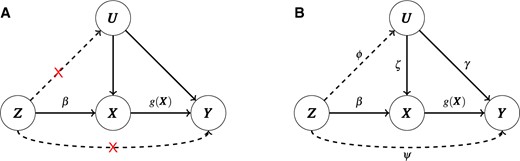
A diagram illustrating the true causal model (A) with all the three valid IV assumptions satisfied or (B) with the exclusion and exchangeability assumptions violated.
2.2. DeepIV
In stage 1, if all three IV assumptions hold, we have |$\boldsymbol{X}|\boldsymbol{Z} \sim N(\boldsymbol{Z\beta}, \sigma^2_{\boldsymbol{X}} \boldsymbol{I}_n)$| by (2.1), where |$\sigma^2_{\boldsymbol{X}} = \sigma^2_{\boldsymbol{U}} + \sigma^2_1$|, and we fit a linear model to have |$\hat{\boldsymbol{\mu}}_{\boldsymbol{Z}} = \boldsymbol{Z\hat{\beta}}$| and |$\hat{\sigma}_{\boldsymbol{X}}^2 = ||\hat{\boldsymbol{\mu}}_{\boldsymbol{Z}} - \boldsymbol{X}||^2_2 / n$| with |$n$| being the sample size in stage 1. Then, |$\hat{F}(\boldsymbol{X}|\boldsymbol{Z})$| is simply |$N(\hat{\boldsymbol{\mu}}_{\boldsymbol{Z}},\hat{\sigma}_{\boldsymbol{X}}^2)$|, from which we can easily sample.
In DeepIV, the interest lies in estimating |$g(\boldsymbol{X})$| given an estimate of |$F(\boldsymbol{X}|\boldsymbol{Z})$|. Its estimating equation corresponds to the Fredholm integral equation of the first kind, which is a notorious ill-posed problem (Kress and others, 1989). This ill-posed inverse problem implies that consistent estimation of |$F(\boldsymbol{X}|\boldsymbol{Z})$| and |$E(\boldsymbol{Y}|\boldsymbol{Z})$| does not necessarily yield a consistent estimator of |$g(\boldsymbol{X})$| (Newey, 2013). Note that the cause of the ill-posed inverse problem is due to estimating |$g(\boldsymbol{X})$| through solving the integral equation (2.3), hence not only DeepIV but also other similar nonparametric IV methods would suffer from it. Regularization methods were proposed to overcome the problem, but the effectiveness depends on specific implementation, which is particularly difficult for DL due to its many hyperparameters and high computational cost. Newey (2013) also showed that it is challenging to estimate the nonlinear effects; in a special case of series approximation (one of the regularization methods), the variance of the estimator was inversely proportional to the IV strengths (i.e., correlation between the IVs and |$\boldsymbol{X}$|); that is, the weaker the IVs, the larger the variance of |$\hat{g}(\boldsymbol{X})$|. For our problem of TWAS, as an overwhelming majority, if not all, of the SNPs (as IVs) are only weakly correlated with |$\boldsymbol{X}$|, the estimation instability is expected to be exacerbated.
High computational cost is another issue when the sample size is large since the training time is further prolonged with the increased training sample size by repeated MC sampling for any given nontrivial network structure. To obtain a reasonably accurate estimate of the integral, we usually need to draw at least dozens of MC samples for a single training sample, which quickly becomes problematic with a typical sample size of TWAS in tens to hundreds of thousands.
2.3. New method: DeLIVR
In this section, we present a new DL-based IV regression method, called DeLIVR, as an alternative to DeepIV, circumventing the two major shortcomings of DeepIV by directly estimating, and subsequently making inference with, |$\hat{E}(g(\boldsymbol{X})|\boldsymbol{Z})$|. That is, we estimate |$E(g(\boldsymbol{X})|\boldsymbol{Z})$| directly without estimating |$g(\boldsymbol{X})$|. Let |$\hat{h}_{\theta}$| be a neural network taking |$\hat{\boldsymbol{\mu}}_{\boldsymbol{Z}} = \hat{E}(\boldsymbol{X}|\boldsymbol{Z}) = Z\hat{\beta}$| as input, we use |$\hat{h}_{\theta}(\hat{\boldsymbol{\mu}}_{\boldsymbol{Z}})$| as the estimate for |$E(g(\boldsymbol{X})|\boldsymbol{Z})$|.
We will show next that if the goal is to uncover whether there is a causal relationship between the exposure |$\boldsymbol{X}$| and the outcome |$\boldsymbol{Y}$|, then estimating |$g(\boldsymbol{X})$| would not be necessary. Instead, based on the following results, directly estimating |$E(g(\boldsymbol{X})|\boldsymbol{Z})$| as a function of |${\boldsymbol{\mu}}_{\boldsymbol{Z}}$| would be effective to answer the question.
Suppose |$X|Z \sim N(\mu_Z, \sigma^2)$| with unknown |$\mu_Z$| in a region containing an open interval and |$\sigma^2$| being a known constant, and |$g(X)$| is a univariate function in |$X$| (and independent of |$\mu_Z$|), then
|$E(g(X)|Z)=c$| if and only |$g(X)=c$|, a constant (almost surely, a.s.).
|$E(g(X)|Z)$| is linear in |$\mu_Z$| if and only if |$g(X)$| is linear in |$X$| (a.s.).
|$E(g(X)|Z)$| is a |$k$|th degree polynomial in |$\mu_Z$| if and only if |$g(X)$| is a |$k$|th degree polynomial in |$\mu_Z$| (a.s.).
The proof of the proposition can be found in the Supplementary material available at Biostatistics online. Here are two simple examples: |$E(X^2|Z)=\mu_Z^2+ \sigma^2$| and |$E(X^3|Z)=\mu_Z^3 + 3\mu_Z \sigma^2$|. A few more examples to contrast |$g(X)$| and |$E(g(X)|Z)$| are given in Table S1 of the Supplementary material available at Biostatistics online. In addition to the normal distribution as used throughout, the proposition may hold for other distributions in the exponential family (as shown in the proof); if we consider only the sufficient condition, then it may hold for other location-scale distributions such as the gamma distribution with |$\beta$| fixed and |$\boldsymbol{\mu}_{\boldsymbol{Z}} = \alpha_{\boldsymbol{Z}} \beta$| as shown in Table S1 of the Supplementary material available at Biostatistics online. Although the proposition (and thus DeLIVR) relies on the parametric assumption on |$F(\boldsymbol{X}|\boldsymbol{Z})$|, DeepIV is no exception in that it requires a specific distribution to implement its MC sampling; further distributional assumptions (e.g., a distribution in the exponential family) are needed for model identification for DeepIV and other related nonparametric IV regression methods (Newey, 2013).
The above proposition lends theoretical support for directly inferring |$E(g(\boldsymbol{X})|\boldsymbol{Z})$|, instead of |$g(\boldsymbol{X})$|, to detect any association between |$\boldsymbol{X}$| and |$\boldsymbol{Y}$|. Although the sufficient condition can be easily proved, the necessary condition is not obvious and only holds almost surely, requiring the completeness of the distribution, such as the normality (or one from the exponential family as shown in its proof). It is important for the proposition to hold to ensure the validity of making inference using |$E(g(\boldsymbol{X})|\boldsymbol{Z})$|. Otherwise, there might be cases where testing with |$E(g(\boldsymbol{X})|\boldsymbol{Z})$| has no statistical power, for example, |$E(g(\boldsymbol{X})|\boldsymbol{Z})$| is constant in |$\boldsymbol{\mu}_{\boldsymbol{Z}}$| but |$g(\boldsymbol{X})$| is not constant in |$\boldsymbol{X}$|; likewise, there might be cases where controlling the Type I error rates is impossible. Although the first two statements in Proposition 1 are two special cases of the third statement with |$k=0$| and |$k=1,$| respectively, we write them out to emphasize that it is equivalent to use either |$g(\boldsymbol{X})$| or |$E(g(\boldsymbol{X})|\boldsymbol{Z})$| to infer (i) no association, (ii) a linear association, and (iii) a nonlinear polynomial association between |$\boldsymbol{X}$| and |$\boldsymbol{Y}$|, respectively. Furthermore, if |$g(\boldsymbol{X})$| is locally smooth enough to be well approximated by a polynomial and thus by a Taylor expansion, then |$E(g(\boldsymbol{X})|\boldsymbol{Z})$| can be also approximated by a polynomial of the same order, suggesting that the same neural network architecture can be used for both DeepIV and DeLIVR.
We implemented both DeepIV and DeLIVR in Python 3.7.9 with TensorFlow 2.3.0 (Abadi and others, 2015) as a feed-forward neural network with five hidden layers and a skip-layer connecting the inputs to the output; see Section S4 of the Supplementary material available at Biostatistics online for details. The skip-layer was used to explicitly account for linear effects. We used the Adam optimizer (Kingma and Ba, 2015) with the default hyperparameter values. We discuss using a simpler architecture on real data in Section S3 of the Supplementary material available at Biostatistics online.
2.4. TWAS-L and TWAS-LQ
2.5. Hypothesis testing
In this section, we introduce hypothesis testing for discovering potential causal relations. Motivated by Chernozhukov and others (2018), we perform hypothesis testing on an independent test set, mainly to avoid possible pitfalls with over-fitted DL models with the training data. Let |$\boldsymbol{Z}$| be the IVs of the gene in an independent test set, and |$\hat{E}(g(\boldsymbol{X})|\boldsymbol{Z})$| be the estimated conditional mean of |$g(\boldsymbol{X})$| given |$\boldsymbol{Z}$|. We want to perform the following two tests,
- Global test: On the test set, we fitwhere |$\boldsymbol{\epsilon}_{G} \sim N(\mathbf{0}, \sigma^2_G \boldsymbol{I}_n)$| is the independent error term, then test |$ H_0:\beta=0 \ vs. \ H_1:\beta\neq 0. $|(2.7)$$\begin{align} {\boldsymbol{Y} = \alpha+\beta \ \hat{E}(g(\boldsymbol{X}) | \boldsymbol{Z}) + \boldsymbol{\epsilon}_{G}} , \end{align}$$
- Nonlinearity test: On the test set, we first fitwhere |$\boldsymbol{\epsilon}_{NL} \sim N(\mathbf{0}, \sigma^2_{NL}\boldsymbol{I}_n)$| is the independent error term, then test |$ H_0:{\beta}_2=0 \ vs. \ H_1:{\beta}_2\neq 0. $|(2.8)$$\begin{align} {\boldsymbol{Y} = \alpha+\beta_1 \ \hat{E}(\boldsymbol{X}|\boldsymbol{Z}) + \beta_2 \ \hat{E}(g(\boldsymbol{X}) | \boldsymbol{Z}) + \boldsymbol{\epsilon}_{NL}}, \end{align}$$
Note that we can do similar tests for TWAS-LQ, with the global test being the F-test on both the linear and quadratic terms, while the nonlinearity test on only the quadratic term. TWAS-L can only test for linearity.
2.6. Combining p-values
Since we need an independent test set to perform hypothesis testing, we have to partition the given data set into two parts as the training and the test data respectively, but the results may vary with different data partitions. In addition, as shown in Kim and others (2015), hyperparameters tuned for estimation may not be optimal for testing. Therefore, it is better to train the model multiple times with different hyperparameters and data partitions then combine the p-values using some methods as described in Liu and Xie (2020) and Hommel (1983), to which we will refer as the Cauchy Combination Test and Hommel’s method, respectively.
The Cauchy Combination Test statistic is calculated as |$T = \sum_{i=1}^{d} \omega_i \tan\{(0.5 - p_i) \pi\}$|, where |$d$| is the total number of runs, |$p_i$| are the p-values, and |$\sum_{i=1}^{d} \omega_i = 1$| are the weights. We will use |$\omega_i = 1/d$|. The combined p-value then is |$ p = 1/2 - (\arctan T)/\pi$|.
For Hommel’s method, let |$\alpha$| be the significance level, |$p_{(k)}$| be the ordered p-values, and |$C_d = \sum_{i=1}^{d} 1/i$|. Then we reject the null hypothesis if there exists at least one |$k$| such that |$ p_{(k)} \leq \frac{1}{C_d} \cdot \frac{k}{d} \cdot \alpha, \quad k = 1,\dots d. $|
2.7. Robust inference on nonlinear causal effects
The idea is that by projecting onto the orthogonal complement of |$\mathrm{Im}(\boldsymbol{Z}_*)$|, we remove any linear direct/pleiotropic effects of |$\boldsymbol{Z}$|, thus bypassing the effects of invalid IVs. Note that this only allows us to test for nonlinear relationships between |$\boldsymbol{X}$| and |$\boldsymbol{Y}$|, especially those cannot be approximated well by a linear function. If |$g(\boldsymbol{X})$| is linear or approximately linear, we do not expect this method to have much statistical power.
In the above robust test, we use the fitted DeLIVR model |$\hat{h}_\theta$| that is trained without accounting for invalid IVs. Alternatively, we can train a robust DeLIVR model, called rDeLIVR, in the projected space (orthogonal to the column space of |$\boldsymbol{Z}_*$|), thus accounting for invalid IVs (with linear direct effects), then conducting hypothesis testing as before. Since, it performed similarly to the (simpler) robust test in simulations, we skip its detailed discussion.
2.8. Real data
GTEx eQTL data. We used the GTEx v8 whole blood gene expression and SNP data in stage 1, which consists of 670 individuals and 20 315 genes. To remove the effects of some covariates (and latent factors from data normalization), we regressed the gene expression (|$\boldsymbol{X}$|) on 68 covariates, then used the standardized residuals as the new |$\boldsymbol{X}$|. For each gene, we extracted the SNPs from its cis-region by expanding 100 kb upstream and downstream its coding region. SNPs with minor allele frequency (MAF) |$\leq$| 0.05 or missing values were also excluded. We further pruned the SNPs so that the absolute value of the pairwise Pearson correlation between any two SNPs was less than 0.8. If the number of SNPs was still larger than 50 after pruning, we would keep the top 50 SNPs with the highest correlations (in their absolute values) with the gene’s expression levels |$\boldsymbol{X}$|. Next, we normalized the data and used backward selection with AIC as the criterion to select SNPs. The final model would be a linear regression model given by the backward selection procedure. If the final model had fewer than two SNPs, then the gene would not be included in the subsequent analysis. For each gene, the F-test was also performed to assess the fit of the final model; if the F statistic was |$\le 10$|, the gene was discarded (i.e., not used in the subsequent analysis) to avoid biases from weak IVs. Note that for TWAS-LQ, we had two stage 1 models (2.5). Therefore, in order to perform both global and nonlinearity test, we required the F statistics for both stage 1 models to be |$\geq 10$|. Otherwise, the gene was discarded for TWAS-LQ.
UKBiobank GWAS data. For stage 2 analysis, we used HDL and LDL cholesterol as the traits. Only the data from the individuals of white British ancestry were used. Any individual who might be a close relative of another was also removed. The number of individuals varies across genes (with a median of 200 000), so any gene with fewer than 500 individuals was removed. After screening, 4701 genes were included in stage 2. Next, we imputed the gene expression using the (estimated) regression coefficients obtained from the GTEx data to obtain |$\hat{\boldsymbol{\mu}}_{\boldsymbol{Z}}$|, then fitted the models (DeLIVR, DeepIV, and the two TWAS models) as described in Section 2. For each gene, the data were divided into the nonoverlapping training, validation and test sets with a ratio of 5:1:4, 4:1:5, or 3:1:6 for DeLIVR and DeepIV. We used the training set to estimate |$E(g(\boldsymbol{X})|\boldsymbol{Z})$| and |$g(\boldsymbol{X})$|, then the test set to perform hypothesis testing described in Section 2.5. The validation set was used to tune hyperparameters of the models. To account for the variation of the model and data partition, we first trained the DeLIVR model with three different data partitions, hyperparameters, and initializations. Then, for those genes with small Cauchy p-values (of the same order of magnitude as the Bonferroni adjusted cutoff) or identified by TWAS-L, we repeated the training process for 21 more times (7 times for each sample splitting ratio) and then used both the Cauchy Combination Test and Hommel’s method to select significant genes (|$p \leq 0.05/4701$|). For DeepIV, the data partition ratio was the same, but we only trained it on the significant genes identified by DeLIVR due to its long running time. To study the power difference due to testing on a fraction of the data, we also ran TWAS-L on only the test sets (ignoring the training and validation set). Additionally, we combined the p-values of TWAS-L on test data with those of DeLIVR to improve the power of DeLIVR.
3. Simulations
3.1. Simulation set-ups
We address two problems in the simulation study. First, we compare the Type I error rate and the power of DeLIVR to those of DeepIV and the parametric TWAS methods, namely TWAS-L and TWAS-LQ, introduced in Section 2. We also demonstrate the flexibility of DeLIVR and DeepIV to estimate |$E(g(\boldsymbol{X})|\boldsymbol{Z})$| with more complex functional forms since we need to estimate |$E(g(\boldsymbol{X})|\boldsymbol{Z})$| for hypothesis testing. Note that DeepIV aims to estimate |$g(\boldsymbol{X})$| and therefore |$E(g(\boldsymbol{X})|\boldsymbol{Z})$| is estimated by MC simulations. Second, we assess the power of the proposed robust test on detecting nonlinear relationships in the presence of invalid IVs with both uncorrelated and correlated pleiotropy.
Next, we describe the simulation setup for the robust test. We selected the invalid IVs (SNPs) as follows: let |$m$| be the number of SNPs, |$\mathcal{I}_k \subseteq \{1,\dots,m\}$| be the set of indices for |$k$| invalid IVs. We first selected |$\mathcal{I}_1$| at random, then for |$k\geq2$|, |$\mathcal{I}_k = \mathcal{I}_{k-1} \bigcup \{i\}$|, where |$i \in \{1,\dots,m\}/\mathcal{I}_{k-1}$| was selected randomly. For gene CDK2AP1, |$m = 2$| so we only ran the simulations for |$k = 1$| invalid IV. For gene NT5DC2, |$m = 6$| so we ran for |$k = 1, 2, \text{ and } 3$| invalid IVs. Once the invalid IVs were selected, for both correlated and uncorrelated pleiotropy, we generated |$\boldsymbol{\psi}, \boldsymbol{\phi} \stackrel{iid}{\sim} N(\boldsymbol{0}, {0.01}*\boldsymbol{I}_k)$|, |$\boldsymbol{U} = \boldsymbol{Z}_{\mathcal{I}_k}\boldsymbol{\phi} + \boldsymbol{\epsilon}_{\boldsymbol{U}}$|, |$\boldsymbol{X} = \boldsymbol{Z\hat{\beta}} + \boldsymbol{U} + \boldsymbol{\epsilon_1}$|,|$\boldsymbol{Y} = g(\boldsymbol{X}) + \boldsymbol{Z}_{\mathcal{I}_k} \boldsymbol{\psi} + \boldsymbol{U} + \boldsymbol{\epsilon_2}$|, where |$\boldsymbol{Z}_{\mathcal{I}_k}$| was the matrix of |$k$| invalid IVs, |$\boldsymbol{\epsilon}_{\boldsymbol{U}} \sim N(\boldsymbol{0}, 0.7\boldsymbol{I}_n)$|, |$\boldsymbol{\epsilon_1}, \boldsymbol{\epsilon_2} \stackrel{iid}{\sim} N(\boldsymbol{0}, 0.3\boldsymbol{I}_n)$|. For uncorrelated pleiotropy, we set |$\boldsymbol{\phi} = \boldsymbol{0}$|. We repeated the experiment 100 times for each |$g(\boldsymbol{X})$| except the linear case. The invalid IVs remained the same for each repeat—only the data were regenerated.
We also provide the expression and phenotype heritability for each setup as an indicator of the “signal-to-noise ratio.” For expression heritability, we used the coefficient of determination, |$R^2$|, of the stage 1 linear regression model. For phenotype heritability, we only account for the heritability due to the true causal cis-SNPs alone, that is, the heritability is defined as |$\text{Var}(g(\boldsymbol{Z\hat{\beta}}))/\text{Var}(\boldsymbol{Y})$|. Note that here |$\boldsymbol{\hat{\beta}}$| was obtained by TWAS-L on GTEx and used to generate the data, so |$\boldsymbol{Z\hat{\beta}} = E(\boldsymbol{X}|\boldsymbol{Z})$| was the true mean. We report the mean phenotype heritability calculated over 1000 runs in Section S2 of the Supplementary material available at Biostatistics online, which was mostly around 5e|$-$|5 except being about 1.5e|$-$|3 for the cubic models. The expression heritability for all setups was 0.167.
3.2. DeLIVR had higher power than DeepIV
Table 1 shows the Type I error rates and the powers for all methods. All methods could control the Type I error rate at the nominal level of 0.05. DeLIVR and DeepIV had lower power than TWAS-L and TWAS-LQ for the linear case. However, combining the p-values of TWAS-L and DeLIVR improved the power, and for the nonlinear cases, DeLIVR had higher power than the parametric models in spite of the sample splitting, while DeepIV was still lower powered. Note that the phenotype heritability for the cubic case was much higher than that for the linear case, but TWAS-L and TWAS-LQ were still lower powered compared to DeLIVR, even when the true |$g(X)$| could be approximated well by a linear function (e.g., for CDK2AP1). In practice, when the true |$g(\boldsymbol{X})$| is unknown, DeLIVR offers more flexibility than parametric models in detecting nonlinear causal effects and is expected to have higher power than DeepIV.
| TWAS-L | TWAS-LQ | DeLIVR | DeLIVR + TWAS-L | DeepIV | ||||||||||
|---|---|---|---|---|---|---|---|---|---|---|---|---|---|---|
| Gene | Global | Nonlinear | Global | Nonlinear | Global | Global | Nonlinear | |||||||
| CDK2AP1 | Null | 0.06 (0.05) | 0.05 (0.05) | 0.05 (0.05) | 0.05 | 0.05 | 0.05 | 0.08 | 0.07 | |||||
| Linear | 0.98 (0.95) | 0.92 (0.91) | 0.04 (0.07) | 0.78 | 0.01 | 0.84 | 0.49 | 0.02 | ||||||
| Quadratic | 0.06 (0.09) | 0.55 (0.53) | 0.64 (0.62) | 0.64 | 0.57 | 0.63 | 0.27 | 0.24 | ||||||
| Cubic | 0.91 (0.87) | 0.84 (0.78) | 0.07 (0.09) | 1.0 | 0.95 | 1.0 | 0.84 | 0.51 | ||||||
| NT5DC2 | Null | 0.05 (0.05) | 0.03 (0.06) | 0.04 (0.06) | 0.05 | 0.04 | 0.05 | 0.05 | 0.04 | |||||
| Linear | 0.93 (0.90) | 0.88 (0.85) | 0.05 (0.06) | 0.69 | 0 | 0.77 | 0.33 | 0.05 | ||||||
| Quadratic | 0.13 (0.14) | 0.84 (0.81) | 0.88 (0.84) | 0.81 | 0.71 | 0.81 | 0.42 | 0.37 | ||||||
| Cubic | 0.13 (0.14) | 0.15 (0.16) | 0.10 (0.12) | 0.47 | 0.37 | 0.45 | 0.08 | 0.04 | ||||||
3.3. DeLIVR provided more accurate and stable estimates of E(g(X)|Z) than DeepIV
Figure 2 shows the fitted models of DeLIVR and DeepIV for gene NT5DC2. The black dashed lines are the true |$E(g(\boldsymbol{X})|\boldsymbol{Z})$| as a function of |$\boldsymbol{\mu}_{\boldsymbol{Z}}$|, and the grey points are |$\boldsymbol{Y}$| for each unique value of |$\hat{\boldsymbol{\mu}}_{\boldsymbol{Z}}$|. The red dashed lines are the average of |$\hat{E}(g(\boldsymbol{X})|\boldsymbol{Z})$| over 100 runs given by DeLIVR. The red shaded area is the “empirical point-wise confidence intervals”—the 97.5th and 2.5th percentiles from the 100 runs. The estimates for DeepIV were calculated by MC simulations. DeLIVR was almost unbiased for the true |$E(g(\boldsymbol{X})|\boldsymbol{Z})$|. On the other hand, DeepIV could only capture the general shape of the true function, and the estimates were very unstable with large variability, even after averaging over 100 runs, which explained its low power.
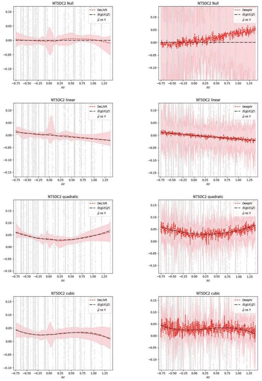
Estimates of |$E(g(\boldsymbol{X})|\boldsymbol{Z})$| given by DeLIVR left) and DeepIV (right): the dash-dotted line is the true |$E(g(\boldsymbol{X})|\boldsymbol{Z})$|; the dashed line is the average of |$\hat{E}(g(\boldsymbol{X})|\boldsymbol{Z})$| over 100 runs; the shaded area is the empirical point wise |$95\%$| CI of |$\hat{E}(g(\boldsymbol{X})|\boldsymbol{Z})$|.
Section S2 of the Supplementary material available at Biostatistics online presents the results for gene CDK2AP1 and the estimated |$g(\boldsymbol{X})$| given by DeepIV.
3.4. Robust test of DeLIVR maintained correct Type I errors in the presence of invalid IVs
Table 2 shows the Type I error rates and power of the robust test of DeLIVR for gene NT5DC2 with both uncorrelated and correlated pleiotropy. DeLIVR could control the Type I error rate at the nominal level of 0.05 with the robust test whereas the default nonlinearity test had dramatically inflated Type I error rates of nearly 1 if there were any invalid IVs. On the other hand, we observed slightly decreasing power of the robust test as the number of invalid IVs increased.
| Models | DeLIVR | ||||||||||||
|---|---|---|---|---|---|---|---|---|---|---|---|---|---|
| No. of invalid IVs | 0 | 1 | 2 | 3 | |||||||||
| Horizontal pleiotropy | Tests | Nonlinear | Robust | Nonlinear | Robust | Nonlinear | Robust | nonlinear | robust | ||||
| Correlated and uncorrelated | Null | 0.03 | 0.07 | 0.84 | 0.07 | 0.99 | 0.03 | .96 | .05 | ||||
| Linear | 0.01 | 0.03 | — | 0.08 | — | 0.09 | - | .06 | |||||
| Quadratic | 0.74 | 0.52 | — | 0.60 | — | 0.47 | - | .34 | |||||
| Cubic | 0.47 | 0.59 | — | 0.38 | — | 0.33 | - | .40 | |||||
| Uncorrelated | Null | 0.04 | 0.08 | 0.86 | 0.06 | 0.88 | 0.07 | .98 | .07 | ||||
| Linear | 0.02 | 0.06 | — | 0.01 | — | 0.06 | - | .02 | |||||
| Quadratic | 0.80 | 0.57 | — | 0.62 | — | 0.51 | - | .27 | |||||
| Cubic | 0.45 | 0.53 | — | 0.31 | — | 0.23 | - | .14 | |||||
When there was no invalid IV, the robust test lost power, as compared to the (default) nonlinearity test, in the quadratic case but not necessarily in the cubic case. The results for rDeLIVR and CDK2AP1 were similar and thus relegated to Section S2 of the Supplementary material available at Biostatistics online.
3.5. Results for PMR-Egger and VC-TWAS
Due to the space limit, we put the results in the Supplementary material available at Biostatistics online. The general conclusions were the same as discussed in the Introduction.
4. Real data: DeLIVR identified additional genes associated with lipids
For real-data analysis, we will only report the results of the Cauchy Combination Test as the significant genes identified by the Hommel’s method were a subset of those identified by the Cauchy Combination Test. The quantile–quantile plot for p-values is shown for TWAS-L and DeLIVR (Figure 3), and we found that the p-values for DeLIVR were better calibrated than TWAS-L. DeepIV did not identify any significant genes for either traits, so we will focus on comparing DeLIVR with TWAS-L and TWAS-LQ. Figure 3 shows the number of significant genes identified for each method. For HDL, TWAS-L discovered 87 significant genes, and with the global test, DeLIVR discovered 58 genes, 49 of which overlapped with those discovered by TWAS-L. Compared to using the entire data set, testing TWAS-L on the test set only identified 58 genes, showing that the power difference between TWAS-L and DeLIVR was mainly due to the difference in the test sample sizes. Additionally, combining the p-values of DeLIVR and TWAS-L on test data improved the number of significant genes to 65, 61 of which overlapped with those identified by TWAS-L. The nonlinearity test for DeLIVR discovered 10 significant genes, 2 of which were identified by the TWAS-L model. TWAS-LQ identified four genes with the global test, one of which was also identified by DeLIVR. As for the nonlinearity test, TWAS-LQ identified two genes, one of which was identified by DeLIVR. There were eight novel genes solely discovered by both the global test and the nonlinearity test of DeLIVR, among which BUD13 was previously found to be associated with HDL. For example, many variants in BUD13 have been found to be related to HDL and other metabolic traits in both European and Asian populations (Johansen and others, 2010; Zhang and others, 2017; Lin and others, 2016; Oh and others, 2020).
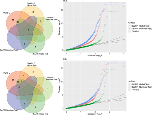
Venn diagrams (left) and Q–Q plots (right) for the numbers of the significant genes for HDL (top) and LDL (bottom); the results of DeLIVR were given by the Cauchy Combination Test over 21 repeated runs for each gene.}
For LDL, TWAS-L discovered 51 significant genes, and with the global test, DeLIVR discovered 40 genes, 29 of which overlap with those discovered by TWAS-L. Testing TWAS-L on the test set identified 35 genes, and combining the p-values of DeLIVR and TWAS-L on test set improved the number of significant genes to 45. The nonlinearity test for DeLIVR discovered 12 significant genes, 5 of which were also identified by TWAS-L. Compared to TWAS-L and TWAS-LQ, the nonlinearity and global test of DeLIVR discovered seven novel genes associated with LDL. Out of the newly identified genes, SLC44A2 and GMIP were identified as significant contributors to the LDL level in many ethnic groups by various studies (Sinnott-Armstrong and others, 2021; De Vries and others, 2019).
The analysis above was based on the assumption that all IVs were valid, which might not be true. Therefore, we applied the robust test in DeLIVR to the significant genes discovered by the nonlinearity test (12 for HDL and 11 for LDL). We used the same Bonferroni corrected cutoff as before (|$0.05/4701 = 1.1\mathrm{e}-5$|). For HDL, none of the genes were significant, though gene BUD13 on chromosome 11 was almost significant with a p-value of |$3.6\mathrm{e}-4$|. For LDL, MAU2 and YJEFN3 on chromosome 19 were significant with p-values of |$6.8\mathrm{e}-14$| and |$2.3\mathrm{e}-7$|, respectively. The plots for the fitted models of these genes are given in Section S3 of the Supplementary material available at Biostatistics online. We can see that for all three genes, DeLIVR showed some nonlinear trends not captured by TWAS-LQ.
5. Discussion
In this article, we have proposed a DL-based IV regression method, DeLIVR, to discover potentially nonlinear causal effects for a more flexible and nonparametric TWAS analysis. In addition, a general hypothesis testing framework was also proposed, along with a robust test in the presence of invalid IVs. In our simulation study, we found that DeLIVR had much higher power than DeepIV, an existing and perhaps best-known DL-based IV regression method. DeLIVR also outperformed the existing TWAS models, such as TWAS-L and TWAS-LQ, when the parametric models were mis-specified. For example, when the true causal relationship between the gene expression/exposure and the trait/outcome was cubic, the nonlinearity test of TWAS-LQ had power of 0.07, dramatically lower than 0.95 of DeLIVR. The simulation study also revealed that DeepIV was unstable in estimating the true causal function |$g(\boldsymbol{X})$|, leading to its low statistical power. Applying DeLIVR to the GTEx and UK Biobank data led to some new discoveries. For example, DeLIVR identified eight genes associated nonlinearly with HDL, which were missed by both parametric TWAS-L, TWAS-LQ, and nonparametric DeepIV. Some of these findings were supported by previous studies. For example, out of the newly discovered genes, BUD13 has been reported to have significant associations with HDL (Johansen and others, 2010; Zhang and others, 2017; Lin and others, 2016; Oh and others, 2020). Similarly, DeLIVR uniquely identified seven putative causal genes for LDL, all of which were missed by TWAS-L, TWAS-LQ, and DeepIV. Some of these genes were still deemed significant by the robust test of DeLIVR after accounting for the possible presence of linear pleiotropic effects of invalid IVs.
Although TWAS has been extensively applied in the last few years, we are not aware of any studies aiming to detect the nonlinear causal relationships with a nonparametric method. Some recently proposed methods addressing the nonlinearity issue, such as TWAS-LQ and PolyMR (Sulc and others, 2021), were however parametric, which may lose power when mis-specified as discussed above. On the other hand, an existing popular nonparametric method, DeepIV, was slow and gave unstable estimates when applied to TWAS data, while hypothesis testing was not studied before. We also note that, although we have focused on TWAS, the proposed method can be broadly applied to other problems, especially if the goal is for nonlinear association testing.
There are a few limitations in this study. First, the major innovation of DeLIVR is to estimate |$E(g(\boldsymbol{X})|\boldsymbol{Z})$|, instead of the causal function |$g(\boldsymbol{X})$|, to serve the purpose of association analysis in TWAS. Hence, DeLIVR does not offer an estimate of |$g(\boldsymbol{X})$|, which may be important in some applications. As a result, DeLIVR is more relevant to association testing (e.g., metabolome- or proteome-wide association studies, in addition to TWAS) than to other IV regression problems. Second, DeLIVR is not applicable to the widely available GWAS summary data, as it requires individual-level data to perform the analysis. Third, the robust test in DeLIVR only works if the underlying causal function is highly nonlinear—cannot be well approximated by a linear function; otherwise, we would lose power. It also depends on the assumption of linear pleiotropic effects of SNPs on a trait, which is however reasonable given small effect sizes of SNPs on complex traits and/or often a small sample size in stage 1, though it is possible and interesting to extend it to nonlinear. Finally, while the power of DL is for multivariate data, we have only considered univariate TWAS with a single gene (or exposure); extensions to multivariate TWAS (or multivariate regression) with multiple genes (or exposures) (Knutson and others, 2020) will be useful.
Data and code availability statement
The GTEx data are available to the approved user at https://www.ncbi.nlm.nih.gov/gap/, and the UKB data are available to the approved user at https://www.ukbiobank.ac.uk/. The R and Python code can be found at https://github.com/RuoyuHe/DeLIVR. For a gene with a total sample size of 200 000, it took approximately 90–120 min to run DeLIVR for all 21 repeats on the AMD Rome.
Supplementary material
Supplementary material is available at http://biostatistics.oxfordjournals.org.
Acknowledgments
The authors thank the reviewers for many helpful comments and suggestions.
Conflict of Interest: The authors declare no conflicts of interest.
Funding
National Institutes of Health (NIH) (U01AG073079, R01AG065636, RF1AG067924, R01AG069895, R01AG074858, R01GM126002, and R01HL116720); and The Minnesota Supercomputing Institute (MSI). The Genotype-Tissue Expression (GTEx) Project was supported by the Common Fund of the Office of the Director of the National Institutes of Health, and by National Cancer Institute (NCI), National Human Genome Research Institute (NHGRI), National Heart, Lung, and Blood Institute (NHLBI), National Institute on Drug Abuse (NIDA), National Institute of Mental Health (NIMH), and National Institute of Neurological Disorders and Stroke (NINDS). The data used for the analyses described in this article were obtained from dbGaP Project #26511. The access to the UK Biobank (UKB) data was approved through UKB Application #35107.
References
GTEx Consortium. (
