


Summary
The rich longitudinal individual level data available from electronic health records (EHRs) can be used to examine treatment effect heterogeneity. However, estimating treatment effects using EHR data poses several challenges, including time-varying confounding, repeated and temporally non-aligned measurements of covariates, treatment assignments and outcomes, and loss-to-follow-up due to dropout. Here, we develop the subgroup discovery for longitudinal data algorithm, a tree-based algorithm for discovering subgroups with heterogeneous treatment effects using longitudinal data by combining the generalized interaction tree algorithm, a general data-driven method for subgroup discovery, with longitudinal targeted maximum likelihood estimation. We apply the algorithm to EHR data to discover subgroups of people living with human immunodeficiency virus who are at higher risk of weight gain when receiving dolutegravir (DTG)-containing antiretroviral therapies (ARTs) versus when receiving non-DTG-containing ARTs.
1 Introduction
Dolutegravir (DTG) is an orally administered antiretroviral medication that in combination with other antiretroviral medications has been approved for the treatment of human immunodeficiency virus (HIV) infection (World Health Organization, 2018). DTG-containing antiretroviral therapies (ARTs) have many advantages such as promising treatment efficacy, high medication resistance barrier, and low cost compared with ARTs previously recommended by the World Health Organization (WHO) (NAMSAL ANRS 12313 Study Group, 2019; Phillips and others, 2019; Venter and others, 2019). However, several randomized trials (Calmy and others, 2020; NAMSAL ANRS 12313 Study Group, 2019; Sax and others, 2020; Venter and others, 2019, 2020) and observational studies (Bourgi, Jenkins, and others, 2020; Bourgi, Rebeiro, and others, 2020; Esber and others, 2022; Surial and others, 2021) have found larger average weight gain among people receiving DTG-containing ARTs. Weight gains can have negative consequences among people living with HIV including increased risk of cardiovascular and metabolic diseases as well as other comorbidities (Achhra and others, 2016; Herrin and others, 2016; Kim and others, 2012). A few studies have explored how weight gain differs between subgroups defined by some individual characteristics (Bourgi, Jenkins, and others, 2020; Calmy and others, 2020; Sax and others, 2020; Venter and others, 2020), but all of these studies focused on subgroups that were pre-specified by the investigators and did not attempt data-driven subgroup discovery.
Data-driven discovery of subgroups with heterogeneous treatment effects requires larger sample sizes than estimation of population average treatment effects (Dahabreh and others, 2016). Unlike randomized controlled trials, which are usually powered to detect average treatment effects in the overall population, electronic health records (EHRs) often contain rich longitudinal data collected on a large number of diverse individuals in a “real world” setting. This makes EHRs well suited for more fine-grained treatment effect analyses such as discovering subgroups with heterogeneous treatment effects and estimating long-term effects of sustained treatments. However, treatment effect estimation using EHRs involves several challenges including: (i) EHRs have repeated measures over time, and these measures are not temporally aligned with the number of repeated measures and timing of the measurements often being informative about outcomes; (ii) potential time-varying confounding; and (iii) potentially informative dropout (i.e., individuals that dropout of the EHRs systematically differ from those who do not dropout).
Tree-based methods stratify the covariate space into interpretable subgroups making them ideal for subgroup discovery (Su and others, 2008). In contrast, most other blackbox machine learning algorithms produce completely personalized predictions (rather than subgroup-specific predictions), and are therefore not applicable for subgroup discovery unless the personalized predictions are post-processed to create subgroups. Previous work on tree-based methods for discovering subgroups with differential treatment effects has mostly focused on cross-sectional randomized (Foster and others, 2011; Seibold and others, 2016; Steingrimsson and Yang, 2019; Su and others, 2009) or non-randomized data (Athey and Imbens, 2016; Yang and others, 2022). Additionally, previously proposed tree-based methods for treatment effect estimation with longitudinal data (Su and others, 2011; Wei and others, 2020) cannot handle both non-randomized time-varying treatment assignment and dropout.
In this article, we develop the first tree-based algorithm for discovering subgroups with heterogeneous treatment effects when comparing the effects of time-varying treatments using non-randomized longitudinal data, in the presence of potentially informative dropout (censoring). The algorithm we develop, referred to as the subgroup discovery for longitudinal data (SDLD) algorithm, extends the generalized interaction tree algorithm (Yang and others, 2022) by combining it with longitudinal targeted maximum likelihood estimators (TMLEs) (Petersen and others, 2014; Stitelman and others, 2012; van der Laan and Gruber, 2012; Van der Laan and Rose, 2018; Van der Laan and Rose, 2011; Van Der Laan and Rubin, 2006). The SDLD algorithm recursively splits the covariate space into disjoint subgroups using splitting decisions that are based on maximizing treatment effect heterogeneity as quantified by subgroup-specific TMLEs. TMLEs are doubly robust (Bang and Robins, 2005; Robins and others, 1994), semi-parametric efficient (Stitelman and others, 2012; Van der Laan and Rose, 2018), and, under mild conditions, guarenteed to take values in the support of the outcome. We apply the algorithm to perform the first data-driven discovery of subgroups with differential effect of DTG-containing ARTs on weight using EHRs of people living with HIV in western Kenya.
2 Data structure and target parameter
For , let be a vector of time-dependent covariates (that includes measures of the outcome Yk) measured at time k, Ak be the binary treatment indicator at time k, Ck be an indicator whether a person drops out at time k, and be the outcome at time K + 1. The baseline covariates can include covariates that do not vary over time and baseline values of time-varying covariates. We assume the following time ordering of the data
By the time ordering assumption, each variable has no causal effect on those measured before. For a vector , define , and X without subscript indicates a vector from time 0 to K (i.e., ). We assume that if an individual drops out at time k, all quantities measured after time k are not observed. That is, Ck = 1 implies that , and are not observed.
Let be the vector of potential outcomes (Rubin, 1974; Robins and Greenland, 2000) under intervention on individual i to set the treatment vector to a and to abolish censoring (i.e., intervention to set ). Similarly, let be the potential covariate trajectory of the ith individual under intervention to set the treatment vector to a and to abolish censoring.
Let take values in . Any set defines a subgroup consisting of individuals with . Define the treatment effect contrasting treatment regimes and within subgroup w as . That is, is the subgroup-specific average treatment effect contrasting the treatment regimes and . Our objective is to find mutually exclusive and exhaustive subgroups of where splitting decisions are made to maximize the between subgroup treatment effect difference.
3 Subgroup discovery for longitudinal data (SDLD) algorithm
3.1 Generalized interaction tree algorithm
In this section, we briefly review the generalized interaction tree algorithm that has been used to discover subgroups with heterogeneous treatment effects for cross-sectional randomized trial data (Steingrimsson and Yang, 2019; Su and others, 2009) and cross-sectional observational data (Yang and others, 2022).
The generalized interaction tree algorithm consists of three steps: initial tree building, pruning, and final tree selection. The algorithm starts by splitting the data into an initial tree building dataset and a validation dataset. Algorithm 1 describes the initial tree building process that runs on the initial tree building dataset where the generalized interaction tree algorithm recursively partitions the covariate space into subgroups until a pre-determined stopping criterion is met (e.g., there are too few observations in each subgroup to justify further splitting). At each attempt to partition the covariate space, the algorithm focuses on discovering subgroups that maximize differences between subgroup-specific treatment effect estimators (using some estimator, , of the treatment effect in subgroup w). In Section 3.2, we describe three subgroup-specific treatment effect estimators appropriate for the longitudinal data structures presented in Section 2. For a given subgroup-specific treatment effect estimator , define the splitting criterion for splitting a subgroup (node) w into two exclusive and exhaustive subgroups l and r as
The splitting criterion (3.1) estimates a standardized difference between the treatment effects in the two subgroups l and r. Selecting the subgroups l and r by maximizing the splitting criterion (3.1) results in a split that tries to find the pair of subgroups that have the largest difference in estimated treatment effects (i.e., maximizing estimated between subgroup treatment effect heterogeneity).
Initial tree building process for the SDLD algorithm
1: Define the root node as consisting of all observations. Set the root node as the node under consideration.
2: Define as the j-th component of the baseline covariate vector. In the node under consideration, find all permissible pairs, , that split the covariate space into two groups defined by and , where J is the number of components in the baseline covariate vector.
3: Run through all possible splits in Step 2 and split the node under consideration into two new subgroups based on the split that maximizes the splitting criterion (3.1).
4: If a pre-determined stopping criterion is met, stop the tree building process; otherwise, on every node that is not already split and has not met the stopping criterion, repeat Steps 2-4.
We refer to the result of Algorithm 1 as the initial tree . The initial tree usually substantially overfits to the data and to reduce overfitting a pruning algorithm uses the initial tree building dataset to create a set of subtrees of that are candidates for being the final tree (i.e., the final model). The pruning algorithm is described in detail in Supplementary Appendix A. In short, the pruning algorithm is based on the split complexity, which for a tree ψ is defined as
where is the set of internal nodes, is the value of the splitting criterion for internal node w, is the number of internal nodes, and λ is a positive penalization parameter. The first term in (3.2) is a measure of the treatment effect heterogeneity of the tree and each additional split in the tree is guaranteed to increase (or at least not decrease) the first term. To offset that, the second term penalizes the size of the tree (a measure of the complexity of the model). For a fixed λ, a subtree of the initial tree is said to be an optimal subtree if it maximizes . Varying λ from 0 to results in a sequence of subtrees of different sizes, , that all are optimal for different intervals of λ.
In the original classification and regression tree algorithm for outcome prediction (Breiman and others, 1984), the final tree from the sequence of trees created by the pruning algorithm is selected by optimizing a cross-validated objective function. However, as the true treatment effect is unknown for all individuals (we only observe at most one of the potential outcomes or ), there is no observed treatment effect for each individual to compare the treatment effect predictions to in the cross-validation procedure. Hence, cross-validation cannot be applied directly to select the final tree in the generalized interaction tree algorithm. To overcome that, the generalized interaction tree algorithm selects the final tree by estimating the split complexity on the validation dataset. For a given tree () and a fixed λ, we calculate the validation split complexity by recalculating the split complexity in (3.2) using the validation dataset. The final tree is selected as the tree that maximizes the validation split complexity. For a fixed λ, a split improves the split complexity if the value of the splitting criterion is larger than λ. If there is no treatment effect heterogeneity, the splitting criterion (3.1) follows a distribution. Hence, selecting λ as the quantile of the distribution () implies that split complexity is improved if and only if the null hypothesis of no difference in treatment effect between the nodes l and r is rejected when using the splitting criterion (3.1) as the test statistic and conducting the test at a level α. Based on this, we propose to select λ as a quantile of the distribution.
By implementing the initial tree building, pruning, and final tree selection, the generalized interaction tree algorithm stratifies the covariate space into mutually exclusive and exhaustive subgroups (terminal nodes).
3.2 Subgroup-specific treatment effect estimation
Implementation of the generalized interaction tree algorithm relies on estimating the subgroup-specific treatment effect . In this section, we describe how TMLE can be used to estimate for a treatment regime a.
3.2.1 Identifiability
The following identifiability assumptions are needed for the potential outcome mean to be identifiable (Bang and Robins, 2005; Pearl and Robins, 1995; Robins, 1986):
Consistency: For time k, , and for every individual receiving treatment that has not dropped out of the study, their observed outcome at time k + 1 () is equal to their potential outcome and their observed covariate trajectory is equal to their potential covariate trajectory.
Sequential exchangeability: At time k, , the potential outcomes ( are independent of treatment Ak and censoring status Ck conditional on past treatment and covariate trajectories.
- Positivity: For time k, , and all such that the density ,where is defined as the empty set and . The positivity assumption says that conditional on past treatment and covariate history there is a positive probability of continuing to follow the treatment regime of interest.
Using these assumptions, the potential outcome mean can be written as
or as a series of iterated conditional expectations (Robins, 1986)
3.2.2 Estimation
Before describing the longitudinal TMLE we start by describing inverse probability weighting (IPW) (Robins and Rotnitzky, 1992) and g-computation estimators (Robins, 1986) that are sample analogs of expressions (3.3) and (3.4), respectively. Denote the probability of following the treatment regime of interest at time k, , conditional on observed treatment and covariate history and not having dropped out from the study as
Similarly, denote the probability of not dropping out from the study at time k, , conditional on observed treatment and covariate history as
For simplicity of notation, denote as and as . Define and let be an estimator of using a model for treatment assignment and a model for being censored at each time. Last, let be a prediction from the model for the ith individual (i.e., the predicted probability that the ith individual follows the treatment regime a and is not censored). Using the sample analog of identification result in (3.3), the IPW estimator is given by
If consistently estimates , the IPW estimator is consistent.
The g-computation estimator, sometimes referred to as the iterative conditional expectation estimator (Wen and others, 2021), is calculated by iteratively estimating the conditional expectations in identification result (3.4), where all the estimators for the conditional expectation are restricted to data from subgroup w. That is, the g-computation estimator is implemented using the following steps:
Estimate using data from individuals that did not dropout (i.e., ). Use the estimator to create predictions for each individual with setting their treatment regime to . Denote the predictions by .
Use as a pseudo-outcome and estimate the conditional expectation of conditional on and among those with . Use the estimator to create predictions . Repeat this iterative process until the conditional expectation that is estimated is only conditional on treatment at the baseline visit A0 and the baseline covariates . Denote the resulting predictions by .
The g-computation estimator is calculated as the subgroup average of the predictions .
The g-computation estimator is consistent if all the conditional expectation estimators required for its implementation are consistent.
The longitudinal TMLE is similar to the g-computation estimator described above, but it updates the conditional expectation of the outcome in each iterative conditional expectation model using the treatment regime and dropout information, targeted to reduce bias (Kreif and others, 2017; van der Laan and Gruber, 2012). Specifically, in the first step of obtaining the g-computation estimator, we use an additional “targeting” step where we fit an intercept only model using as the outcome with as an offset and with weights , where the treatment assignment and the probability of being censored at each time are estimated. We denote the resulting predictions by and this targeting step is performed for each iterative conditional expectation. The TMLE estimator is then calculated as the subgroup average of the predictions . In contrast to the IPW and g-computation estimators, TMLE is doubly robust (van der Laan and Gruber, 2012). That is, it is consistent when either (i) all models for the treatment assignment and the dropout probability are correctly specified or (ii) all models for the conditional expectation of the outcome are correctly specified. It is semi-parametric efficient when all the models are correctly specified (van der Laan and Gruber, 2012). TMLE is a substitution estimator, and is therefore, under mild assumptions, guaranteed to fall within the support of the outcome . While we focus on TMLE in the remainder of the manuscript, the IPW, g-computation, or other estimators could be used including the estimator developed in Bang and Robins (2005) that is also doubly robust.
3.3 Subgroup discovery for longitudinal data (SDLD) algorithm
The SDLD algorithm is defined by using the longitudinal TMLE as the treatment effect estimator in the generalized interaction tree algorithm. We implemented the SDLD algorithm using the R package rpart to build the initial tree and we constructed the longitudinal TMLE used in the user-specified splitting rules and node-specific estimators in rpart using the R package ltmle (Lendle and others, 2017). In Supplementary Appendix C, we present simulations that show good finite sample performance of the SDLD algorithm for identifying the correct subgroups. The SDLD algorithm splits the covariate space into disjoint and exhaustive subgroups based on maximizing between subgroup treatment effect heterogeneity and within each subgroup a treatment effect estimator is calculated (terminal node estimator). The following theorem is proved in Supplementary Appendix B.
If Assumptions B.1–B.5 in Supplementary Appendix B hold, the SDLD algorithm is L2 consistent.
At each splitting decision, the SDLD algorithm discovers subgroups by searching over all possible covariate and split-point combinations and selecting the combination that maximizes between subgroup heterogeneity estimated by the splitting criterion (3.1). As a result, the observed treatment effect heterogeneity is likely overestimated and that results in bias in the subgroup-specific treatment effect estimators. Data splitting can be used to get unbiased subgroup-specific treatment effect estimators (Fithian and others, 2014; Yang and others, 2022). Data splitting separates the data into two disjoint and exhaustive parts. One part is used for fitting the SDLD algorithm and producing a list of subgroups and the other part is used for subgroup-specific treatment effect estimation and confidence interval construction. As the data used for subgroup discovery and subgroup-specific treatment effect estimation are independent, the TMLE estimators for the subgroup-specific treatment effect inherit the theoretical properties of the TMLE estimator. The downside of data splitting is the reduced sample size used for both fitting the SDLD algorithm and for estimating subgroup-specific estimators of treatment effect, likely resulting in lower power for detecting subgroups and wider confidence intervals for subgroup-specific treatment effect estimators.
4 Discovering subgroups with differential weight gain when on DTG-containing ARTs versus non-DTG-containing ARTs
DTG is an antiretroviral medication that belongs to the class of integrase strand transfer inhibitors. In combination with other medications, DTG has shown promising results for improving viral suppression in clinical trials and is globally used today (Kandel and Walmsley, 2015). A concern with DTG-containing ARTs has been the emergence of substantial weight gain as a potential side effect. A recent phase III trial conducted in South Africa (Venter and others, 2019, 2020) compared two DTG-containing ARTs with standard of care over a 96-week follow-up period. Substantially higher weight gains were seen in the two groups receiving DTG-containing ARTs compared with the standard of care group. Another phase III trial conducted in Cameroon also showed larger weight gains when on DTG-containing ART compared with a low-dose efavirenz-based ART (Calmy and others, 2020; NAMSAL ANRS 12313 Study Group, 2019). Of particular concern is that weight gain associated with DTG-containing ARTs has been shown to be associated with increased truncal fat, a known risk factor for adverse cardiovascular outcomes among people living with HIV (Lake, 2017).
Not all people are expected to be at the same risk for increased weight gain associated with DTG-containing ARTs. In the South African trial previously described, weight gain was greater for females and people with lower CD4 counts or higher viral loads. Similarly, in the Cameroon trial weight gain was more severe among women. Discovering subgroups of people for whom being on DTG-containing ARTs is more likely to cause substantial weight gain can help the development of treatment recommendations or monitoring plans tailored to a person’s risk profile.
The Academic Model Providing Access to Healthcare (AMPATH) partnership is a consortium of research institutions focusing on prevention and treatment of HIV in western Kenya (Tierney and others, 2007). AMPATH administers the AMPATH’s open-source electronic medical record system (AMRS), which is a large-scale EHR database that has information on clinical encounters, lab measurements, and demographic characteristics. We implemented the SDLD algorithm on data from AMRS to discover subgroups with differential effect of DTG-containing ARTs on weight.
We included people living with HIV who were at least 18 years old, were initiating or on ART, and had data on or after July 1, 2016 in AMRS. For each individual, we defined time 0 as July 1, 2016 if the person was enrolled in AMPATH before that time and as the enrollment date at AMPATH if the person was enrolled after July 1, 2016. To structure the data, we used time periods with a length of 200 days and captured data at time k within days , for (e.g., we used data from days 0 to 199 to create and days 200 to 399 to create ). We focused on the first five time periods (1000 days) as the data on people that were always on DTG-containing ARTs became sparse over time, resulting in unstable estimates over longer follow-up. We censored individuals at time k if there was no clinical visit in the time periods after time k. As pregnancy leads to natural weight gain, we excluded women that were pregnant at baseline and censored individuals at time k – 1 if they were first recorded as pregnant at time k, . We excluded one individual who had a data entry error whose ART start date was recorded before date of birth and individuals that had no outcome or treatment information available in any time period.
Since there are differences in the expected weight gain between individuals who are newly initiating ART and those who are switching ARTs while virally suppressed (Lakey and others, 2013; Guaraldi and others, 2021), we restricted the analysis to patients who were treatment free at time 0. We defined treatment free as patients who were either newly initiating ART at time 0 or had a viral load measurement that is missing or greater than or equal to 200 (i.e., not virally suppressed) at time 0 and did not have a clinical visit in the 200-day period immediately before time 0. This resulted in an analysis set consisting of 62,073 individuals who had a total of 843,287 unique clinical visits.
The outcome of interest was weight in kilograms at time 4 (i.e., Y4 collected within days 800–999). Treatment at each time was defined as 1 if an individual was receiving a DTG-containing ART and 0 if not. The two treatment regimes of interest were always on and never on DTG-containing ART. We included HIV viral load, systolic blood pressure, diastolic blood pressure, weight, height, whether the individual had active tuberculosis, was being treated for tuberculosis, was married or living with partner, and whether the individual was covered by the National Health Insurance Fund as time-dependent covariates. The vector of baseline covariates included the values of time-varying covariates at time 0, gender, age when starting ART, age at time 0, time on ART at time 0, whether the individual was enrolled on or after July 1, 2016, and whether the individual was newly initiating ART or had been on ART 200 days before time 0. Further details on how we pre-processed the data and how we handled missing data and multiple clinic visits within each time period are provided in Supplementary Appendix D.1.
When implementing the SDLD algorithm, we applied data splitting by randomly selecting 60% of the dataset (37,243 individuals) for tree building using the SDLD algorithm and 40% (24,830 individuals) for subgroup-specific treatment effect estimation. In the tree building dataset, we randomly sampled 80% (29,794 individuals) for initial tree building and used the remaining 20% (7,449 individuals) as the validation set used for final tree selection. As the influence curve-based variance estimate for continuous outcomes implemented by the ltmle package may be anti-conservative, we constructed confidence intervals for the subgroup-specific treatment effects using the non-parametric bootstrap with 1,000 bootstrap samples.
Implementing the SDLD algorithm requires estimating models for the probability of treatment assignment, the probability of dropping out of the study, and the estimation of the pseudo-outcome at each time. For all these models, we used generalized linear regression models with linear and additive main effects for all past covariate and treatment variables fitted using only data in the subgroup under consideration.
Figure 1 shows the estimated average weight had all individuals been always or never on DTG-containing ARTs (left) and the average weight gain when comparing always being on DTG-containing ARTs to never being on DTG-containing ARTs (right) at each time. The confidence intervals are estimated using the non-parametric bootstrap with 10,000 bootstrap samples. The numerical values of the estimates and the corresponding confidence intervals used for making Figure 1 and the number of individuals always and never on DTG-containing ARTs at each time are included in Table S4 in Supplementary Appendix D.2. The results show that sustained treatment with a DTG-containing ART leads to increased weight gain compared with never receiving DTG; the estimated weight gain increases from 1.09 kg at time one (i.e., days 200–399) to 1.30 kg at time four (i.e., days 800–999).
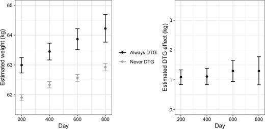
Estimated average weight (left) using TMLE if always and never being on a DTG-containing ART and estimated effect on average weight (right) comparing always versus never being on a DTG-containing ART at each time. Error bars show 95% confidence intervals estimated using the non-parametric bootstrap.
Figure 2 shows the final tree structure produced by the SDLD algorithm with subgroup-specific treatment effect estimates and associated 95% confidence intervals. The final tree splits on gender. The results suggest that the effects of DTG-containing ARTs are larger for females than males (1.98 vs –0.14 kg) although the 95% bootstrap confidence intervals are slightly overlapping ([-1.08, 0.74] for males and [0.69, 3.17] for females). Results from randomized trials and other data sources support the finding that additional weight gains due to being on DTG-containing ARTs are larger among females than males (Bourgi, Jenkins, and others, 2020; Calmy and others, 2020; Sax and others, 2020; Venter and others, 2020).
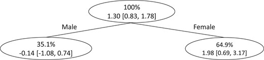
Final tree structure when the SDLD algorithm is applied to data from EHRs on people living with HIV in western Kenya to discover subgroups with heterogeneous effects of DTG-containing ARTs on weight gain. Within each subgroup, the first row shows the percentage of the dataset that belongs to the subgroup and the second row shows the estimated weight gain comparing being always versus never on DTG-containing ARTs and associated 95% confidence interval.
We caution that the subgroup-specific treatment effect estimators only have a causal interpretation if the identifiability and the statistical modeling assumptions are met. A key untestable identifiability assumption is the sequential exchangeability assumption. A recent manuscript (Bourgi and others, 2022) analyzing data on HIV patients in Western Kenya found that gender, CD4 count, weight at baseline, and whether the patient was receiving active tuberculosis therapy were associated with a greater weight gain. In our analysis we account for gender, weight at baseline, viral load, and whether the patient had active tuberculosis. Viral load and whether the patient had active tuberculosis are expected to be highly correlated with CD4 count and whether receiving active tuberculosis therapy, respectively.
Supplementary Appendix D presents additional results including the proportion of underweight and overweight participants across time, distribution of tenofovir disoproxil fumarate containing ARTs when always and never on DTG-containing ARTs, and stability of the SDLD algorithm across data splits. Figure S2 in Supplementary Appendix D compares influence curve based and bootstrap-based confidence intervals and shows that the influence curve-based confidence intervals are much narrower.
In Supplementary Appendix E, we present the analog analysis when the analysis set is not restricted to treatment-free patients. The results are similar to the analysis presented in this section. The final tree from the SDLD algorithm first splits on gender and then makes another split in the female group on whether age at time 0 is less than 42.8 or not. However, the data-split bootstrap-based confidence intervals for younger and older females are highly overlapping. In Supplementary Appendix D, we present the number of times the final tree implemented on the treatment-free analysis set splits on each variable and following gender the variables that are most commonly used for splitting are age at ART initiation and age at time 0.
5 Discussion
We developed the SDLD algorithm for discovering subgroups with heterogeneous treatment effects using longitudinal observational data. The algorithm combines the generalized interaction tree algorithm with longitudinal targeted maximum likelihood estimation and can handle time-varying non-randomized treatment assignment and dropout. We used the algorithm to discover subgroups of individuals with differential weight gain when receiving DTG-containing ARTs using data from AMPATH. Our results suggest that gender is the primary modifier of weight gain from receiving DTG-containing ARTs versus non-DTG-containing ARTs, with females gaining more weight than males. This result is consistent with prior literature where subgroup analyses using pre-specified subgroups (not data-driven subgroup discovery) showed larger weight gains among females.
Our analysis focused on comparing DTG-containing ARTs to other non-DTG-containing ARTs and did not distinguish among different antiretroviral medications included in DTG-containing ARTs. Previous studies have evaluated different DTG-containing ARTs (Venter and others, 2019) and the results show that the weight gains might differ depending on what medications DTG is combined with. Further investigation into specific DTG-containing ARTs might provide a more fine-grained understanding of the effect of DTG on weight gain. When implementing the SDLD algorithm there is a trade-off between identifying spurious subgroups (type I like error) and failing to identify true subgroups (type II like error). That trade-off is largely controlled through the selection of the tuning parameter λ where larger values of λ result in smaller trees (less type I like errors). In the analysis presented in Section 4, we have taken a rather conservative approach by selecting λ as the 95th quantile of the distribution, but if the goal of the analysis is more exploratory a smaller λ value can be used (e.g., the 90th quantile of the distribution).
The SDLD algorithm defines subgroups based on baseline covariates. Extending the algorithm to dynamically update the subgroups when new information becomes available is of interest (Sun and others, 2020). Although our application focuses on always and never receiving DTG-containing ARTs, the SDLD algorithm can accommodate other treatment regimes as well. Furthermore, the SDLD algorithm results in a single tree structure that creates an interpretable treatment effect stratification rule by partitioning the covariate space into identifiable subgroups with differential treatment effects. For computational simplicity, we used generalized linear regression to estimate the nuisance functions required for implementation of the TMLE. But estimating the nuisance functions using the super learner (van der Laan and others, 2007) provides an appealing alternative that allows for more flexible estimation that is less susceptible to model misspecification.
Funding
This work was supported in part by Patient-Centered Outcomes Research Institute (PCORI) awards [ME-2019C3-17875, ME-2021C2-22365]; National Library of Medicine (NLM) grant [R01LM013616]; and National Institute of Allergy and Infectious Diseases (NIAID) awards [P30AI042853, R01AI167694, K24AI134359]. The content is solely the responsibility of the authors and does not necessarily represent the official views of the NLM, NIAID, PCORI, PCORI’s Board of Governors, or PCORI’s Methodology Committee.
Supplementary material
Supplementary material is available at http://biostatistics.oxfordjournals.org.
Because the dataset in Section 4 cannot be made publicly available, we simulated a dataset with similar structure. Details of the simulated dataset and the results we obtained when applying the SDLD algorithm to this dataset are provided in Supplementary Appendix C.3. The simulated dataset, and the R code used to implement the SDLD algorithm on the dataset are available at github.com/jiabei-yang/SDLD.
Conflict of Interest
None declared.
