Multiple imputation of more than one environmental exposure with nondifferential measurement error

Summary

1 Introduction

Prevalence of allergic disease and asthma among children is increasing worldwide. Sensitization to indoor allergens increases the risk of asthma morbidity. Sensitization to multiple allergens is common among asthmatic children. Exposure to multiple allergens may produce larger health effects than would be predicted based on each allergen, and thus it is important to study the coexposure to allergen mixtures on asthma morbidity. However, the measures of indoor allergen concentrations are often subject to measurement error (Daly and others, 2005) that distort statistical inferences (Wald, 1940), leading to flawed scientific conclusions. Specifically, regression coefficients of variables subject to measurement error are often attenuated (Thomas and others, 1993; Marshall and Hastrup, 1996; Pollack and others, 2012; Keogh and others, 2020), and effects of other variables are subject to bias when variables subject to measurement error are included as covariates (Marshall and others, 1999).

This article is motivated by the Neighborhood Asthma and Allergy Study (NAAS) for assessing the associations between coexposure to multiple indoor allergens and the exhaled nitric oxide level, a test for asthma diagnosis and management, of 7–8 years old asthmatic children in New York City. Homes of participating families were visited during which a detailed questionnaire was administered, and a dust sample was collected from the child’s bed. The indoor allergens in the dust samples were measured by immunoassays that are subject to measurement error. To correct for this, calibration data that measure both true and estimated concentrations of the allergens are needed. In the NAAS, such calibration data are available from the standard samples of the same immunoassay plates used for measuring the indoor allergens of the NAAS samples. Specifically, standard samples with known allergen concentrations are diluted, and the estimated allergen concentrations are recorded. Because the calibration data only contain the true and measured concentrations of allergens, this is an external calibration problem (Pauls and McCoy, 1986). For internal calibration, the calibration data also contain information of other variables.

The literature on covariate measurement error has largely concerned the case of a single exposure (Keogh and Bartlett, 2021; Guo and others, 2012; Messer and Natarajan, 2008; Pollack and others, 2012). To correct for the measurement error in immunoassays, the classical calibration (CC) method is often used (Higgins and others, 1998). The standards data are first used to create a calibration curve relating measurements to the true concentrations, and the estimated concentration of new samples are then read off from the calibration curve. Another commonly used method with external calibration is the external regression calibration (RC) (Spiegelman and others, 2001) or regression prediction (RP) (Guo and others, 2012), which regresses the true concentrations to the measurements in the standards and then predicts the concentrations of the new samples. However, when the measurement error is substantial, both CC and RP are biased (Keogh and Bartlett, 2021; Guo and others, 2012). Alternatively, Guo and Little (2011) apply multiple imputation (MI) for missing data to accommodate measurement error in such settings.

Regression models with a set of correlated covariates with measurement error are less studied. In this article, we propose a constrained chained equations multiple imputation (CEMI) method, in which we treat the true concentrations in the main study sample as missing and utilize MI to fill in these values. Standard MI algorithms without constraints do not work with external calibration, because there is insufficient information to estimate all the imputation model parameters (Guo and Little, 2011). Our constrained CEMI method addresses this problem by exploiting parameter restrictions based on strong nondifferential measurement error (NDME) assumptions. We assume that the measurement error is independent of the outcome and the other covariates in the model, given the true values of the exposures, and is reasonable in our study. This assumption is stronger than the usual NDME assumption, which assumes the measurement error is independent of the outcome given the true values of the exposures and other error-free covariates. We show in simulations that with external calibration the constrained CEMI method outperforms CC and RP in estimating regression coefficients, and when standard errors are estimated by the bootstrapped MI method it yields confidence intervals (CIs) with closer to the nominal level coverage. We further extend the constrained CEMI method to the setting where some of exposure measures are only known to be below some thresholds or limits of detection (LODs).

2 Methods

2.1 Background

We consider data structures displayed in Figure 1, where Y denotes a response variable, $X=(X1,X2,…,Xp)T$ denotes the true value of p exposures, $W=(W1,W2,…,Wp)T$ are the corresponding error-prone measures of X, and Z denotes other covariates, assumed to be measured without error. The blanks in Figure 1 denote unobserved values. Information about the measurement error is contained in calibration data with measured and true values of the exposures both recorded. We call the calibration data internal when they are a random sample from the main study, as in Figure 1c. We call the calibration data external when they are from another source, where information of Y and Z are not available. Figure 1 shows two external calibration scenarios. In Figure 1a, the multiple exposures share the same calibration data. In Figure 1b, each X variable has its own calibration data and the correlations between X’s are not observed. Figure 1d and e are special cases of Figure 1a and b, respectively, in which some of the measures of W in the main study sample are below LODs.

Fig. 1

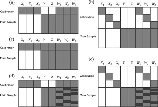
Three study designs using calibration data for correcting measurement errors in the main study sample: (a) external design with common calibration data for all Xs, (b) external design with different calibration data for each X, (c) internal design, and (d), (e) external design with common or different calibration data but some measures in W in the main study sample are below LODs. The gray areas denote observed data, the blanks denote missing data, and the black areas denote data below LODs.

Open in new tabDownload slide

To estimate the β coefficients in model (2.1), commonly used methods for regression with covariates subject to measurement error include the method that ignores measurement error (naive regression), the CC method, and the RP method under external calibration or the RC method under internal calibration. The naive method ignores the measurement error and uses the coefficients of the error-prone covariate W to estimate the coefficients of X in the regression of Y on X given Z.

The β coefficients in model (2.1) are then estimated by fitting regression of Y on $X^mainCC=(X^main,1CC,…,X^main,pCC)$ and Z, computed on the main study data. The CC method is biased when the measurement error is nontrivial.

The β coefficients in model (2.1) are then estimated by fitting regression of Y on $X^mainRP=(X^main,1RP,…,X^main,pRP)$ and Z, based on the main study sample. The RP method requires X does not depend on Y or Z. It corresponds to the RC method when there are no covariates Z. Under the internal calibration in Figure 1c, the RC method is used instead by regressing each X on both the corresponding W and Z.

2.2 Constrained chained equations multiple imputation

An alternative approach for measurement error is to use MI to fill in the missing data in the main study and calibration samples, and in particular X in the main study sample by assuming data are missing at random (MAR) (Cole and others, 2006; Guo and Little, 2011). Chained equations algorithms provide a flexible set of methods for the multivariate MI. See in particular the mice package in R (van Buuren and Groothuis-Oudshoorn, 2011), the mi command in Stata (StataCorp, 2021), and the SAS/R/Stata callable independent software IVEware (Raghunathan and others, 2001). The chained equations approach proceeds with the imputation of one variable at a time, by fitting a model with the variable to be imputed as the dependent variable and the other variables in the data set as the independent variables. Once a variable is imputed, both the observed and imputed values of this variable are utilized in the imputation of others. The imputation process continues until all missing data are imputed, and the procedure is iterated. The entire imputation process is repeated M times to obtain M complete data sets each from the cycles of the chained equation process. Although the imputation models are not necessarily Bayesian, Bayesian models are attractive in allowing uncertainty in the parameter estimation of imputation models and yielding proper imputations of missing values (Rubin, 1987).

Chained equations MI requires modification in the setting of measurement error with external calibration, because the information from calibration samples is insufficient to identify the model parameters. Strong NDME assumptions are used to overcome this challenge. For the external calibration design in Figure 1a, because Y and Z are not measured in the calibration sample, we assume that each exposure W_j does not depend on the outcome Y or the error-free covariates Z, given the true values of all the elements of the exposures X (strong NDME Assumption S1). For the external calibration design in Figure 1b, we need an even stronger assumption because each exposure uses separate calibration samples. We assume that W_j is independent of not only Y and Z but also other ${Xk,k≠j}$ given X_j (strong NDME Assumption S2). Both assumptions are stronger than the usual NDME assumption, which assumes the error-prone measures do not depend on the outcome, given the true values of the exposures and the error-free covariates (Carroll and others, 2016). The strongest NDME Assumption S2 is reasonable for the immunoassays data with measurement error due to biological variation in our NAAS application.

To implement the constrained CEMI method, the calibration samples are first concatenated with the main study sample to obtain data with one of the structures as shown in Figure 1. The chained equations algorithm is applied assuming data are MAR with constraints on the regression parameters of the imputation models implied by the strong NDME assumptions. With the external design in Figure 1a, the strong NDME Assumption S1 implies that the distribution of Y and Z only depends on X but not W. Figure 2a shows the imputation matrix for the constrained CEMI under this design, in which rows correspond to the variables to be imputed and columns correspond to the predictors of the imputation models. In each iterate of the chained equations process, an imputation model is fit for each variable in the rows of the imputation matrix using the variables in the columns with a check mark as the predictors. Variables in the columns without a check mark are excluded, reflecting the constraints imposed on the constrained CEMI. Under this external calibration design, the constraints are only imposed in the imputation models for Y and Z but not for X. We show in Section SA of the supplementary material available at Biostatistics online the steps of one iterate of the constrained CEMI with all variables measured in continuous scale.

Fig. 2

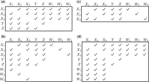
Four imputation matrices, applying constraints of the strong NDME assumptions, used in the constrained CEMI method for correcting measurement errors in the main study sample: (a) external design with a common calibration data for all Xs under the strong NDME Assumption S1, (b) external design with different calibration data for each X under the strong NDME Assumption S2, (c) internal design under the strong NDME Assumption S2, and (d) external design with a common calibration sample and some measures of W in the main study data below LODs under the strong NDME Assumption S1.

Open in new tabDownload slide

For the external calibration design with a different calibration sample for each X in Figure 1b, W and X are not fully observed in all the calibration samples. Figure 2b shows the imputation matrix. With the strong NDME Assumption S2 for this external design, each W only depends on the corresponding X. For example, to impute the missing values of W₁ in the calibration samples not for W₁, we fit a Bayesian linear model of W₁ given X₁ using the calibration sample for W₁ and the observed W₁ and imputed X₁ in the main study sample. The missing W₁ in the calibration samples not for W₁ is then imputed with draws from its posterior predictive distribution given the imputed values of X₁ in its previous iterate. The strong NDME Assumption S2 also implies that the distribution of X₁ depends on X₂, X₃, Y, Z, and W₁ but not on W₂ or W₃. Similar constraints are applied to the imputations of X₂ and X₃.

With external calibration, the calibration data are included in the imputation step, because they contain information that is useful for imputing X in the main study sample. But after imputation, the calibration sample has nothing more to contribute in estimating the regression of $Y∼X+Z$⁠. Actually, the random variation in the imputed Y and Z in the calibration samples add nothing but noise to the estimates (Von Hippel, 2007; Little and Zhang, 2011). Therefore, only the main study sample is used in the postimputation analyses.

Finally, with internal calibration in Figure 1c, Y, Z, and W are fully observed in both the main study sample and the calibration sample. We only need to impute X in the main study sample. Unlike external calibration, the calibration data in internal calibration can be used to improve the estimation of the regression of $Y∼X+Z$ in the postimputation analyses. Therefore, the combined data of the main study and calibration samples should be used in the postimputation analyses, unless the analysis of interest is only on the main study data. The strong NDME assumptions are not required anymore and only the MAR assumption is needed, but the constraints in Figure 2c can be applied to increase efficiency when the postimputation analyses only involve the main study sample and the strong NDME Assumption S2 is reasonable.

2.3 Variance estimation for the constrained CEMI

Rubin’s variance estimation method (Rubin, 1987) for MI data (see Section SB of the supplementary material available at Biostatistics online for details) does not apply under external calibration here, when the calibration and main study data are involved in the imputation but only the main study sample is used in the postimputation analyses. Reiter (2008) showed that Rubin’s variance estimator can have positive bias in this situation, leading to coverage rates for the CIs above the nominal level. Reiter (2008) instead proposed a two-stage imputation procedure to generate imputations that allow for consistent variance estimates. Specifically, m sets of draws for imputation model parameters are obtained in the first stage, and n sets of draws of X are obtained given each set of imputation model parameters in the second stage, yielding $M=m×n$ imputed data sets. The results from the M imputed data sets are then combined using a modified variance combining rule (see Section SC of the supplementary material available at Biostatistics online for details). We found that Reiter’s formula can produce unnecessarily small degrees of freedom associated with a t distribution and very wide CIs, and thus considered other methods for variance estimation.

2.4 Extension to handle measures below LODs

Measures below LOD, also called nondetects, present another challenge to the statistical analysis of allergen concentrations estimated using immunoassays. The data structure is presented in Figure 1d and e for the two external calibration scenarios, in which some measures of W₁, W₂, and W₃ in the main study sample are below LODs. Data below LODs are typically replaced with LOD/2 or LOD/$2$⁠. Although the simple substitution with a constant method is easy to apply, it can result in large bias in both descriptive statistics and analytic inference particularly when the variable concerned is measured on the log scale. Alternatively, multiple imputation can be used to impute data below LODs.

Data below LODs for which the true values are unknown are interval censored, with the true values between 0 and the LOD level. To impute each W in the main study sample, we can use a tobit regression (Tobin, 1956). The constrained CEMI method proceeds by adding one more imputation step. For external calibration in Figure 1d, the updated imputation matrix is shown in Figure 2d. We consider a univariate tobit regression for each W_j, where W_j follows a normal distribution $N(ξ0j+Xξj,σj2)$ with mean $ξ0j+Xξj$ and variance $σj2, j=1,…,p$⁠. Bayesian computation for the tobit regression can be intensive and thus we estimate the model parameters using the maximum likelihood estimation (MLE). The imputed value of W_j for the censored observation is then obtained by draws from the truncated normal distribution with mean and variance of the normal distribution estimated using MLE and the imputed values falling between 0 and LOD. A similar imputation algorithm for nondetects also applies to the external design with separate calibration data in Figure 1e using the imputation matrix in Figure 2b. Because each W_j only depends on X_j under the strong NDME Assumption S2, we consider a univariate tobit regression for each W_j assuming $Wj∼N(ξ0j+ξjXj,τj2)$⁠. We denote the modified constrained CEMI method for handling data below LODs the CCEMI-LOD.

We wrote a custom function in R for implementing the tobit regression imputation for nondetects, which can be utilized within the mice function in R. We include the R code of this custom function and a sample code for implementing the CCEMI-LOD method in our project GitHub.

3 Simulation study

We run 500 simulations for each combination of ρ_xx, ρ_xz, and $σ2$⁠. In each simulation, we generate 300 observations for the main sample and 100 for the calibration sample; We remove X values from the main study sample and also remove (Y, Z) values from the calibration sample in external calibration. We compare the constrained CEMI (CCEMI) method to the naive regression, CC, and RP in external calibration or RC in internal calibration. To access the utility of constraints imposed in the constrained CEMI method, we apply the mice package in R without any constraints on the imputation matrix, that is, including all the available variables as independent variables in the imputation models. We generate 20 imputations for each simulated data and use the default Rubin’s method for variance estimation. We call this the unconstrained CEMI (UCEMI) method. Finally, we include a benchmark estimator (Full), which fits model (3.8) using the true values of X as if they were measured. All the postimputation analyses use the main study data only, except for Simulation 3 under internal calibration, in which the CCEMI and UCEMI are performed first using the combined data of the main study and calibration samples and then on the main study data only.

3.1 Simulation 1: External design with common calibration data

We first consider the external design in Figure 1a, where the three exposures share the same calibration data. Figure 3 shows the violin plots for the estimates of $γ$ coefficients in model (3.8) across the 500 simulations comparing the naive regression, CC, RP, UCEMI, CCEMI, and the benchmark methods. Rows are for each of γ coefficients and columns are for various combinations of $(σ2,ρxx,ρxz)$⁠. The true values of $γ$$(γ1=1.2,γ2=0.8,γ3=0.4,γz=0.4)$ are plotted using horizontal lines. The noncoverage rate (⁠$×1000$⁠) of 95% CI of each estimator is shown on the top of each plot, with 50 being the nominal level. As expected, the naive regression estimates are biased, and empirical noncoverage rates of 95% CIs significantly exceed the nominal level in all simulation scenarios. The CC method also performs poorly, with substantial bias and high noncoverage rate, particularly when the measurement error, $σ2$⁠, is large. The bias also increases with the magnitude of the γ coefficients, with the largest bias observed in estimating γ₁ associated with X₁. RP performs better than the naive and CC methods in estimating the coefficients associated with X but performs poorly in estimating γ_z. Specifically, the RP method yields smaller bias than the naive and CC methods with much better coverage for $(γ1,γ2,γ3)$ when $σ2$⁠, ρ_xx, and ρ_xz are small, but the bias increases and the confidence coverage gets worse as the measurement error and correlations increase. Under all simulation scenarios considered here, the CCEMI method has very small empirical bias and the bootstrapped MI approach for variance estimation yields CIs with coverage rates close to the nominal level for all the $γ$ coefficients. Compared to the benchmark method, the estimates of the CCEMI have similar bias but larger variation.

Fig. 3

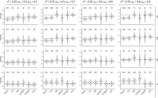
Results in Simulation 1 for the external design with a common calibration data for all X. Each plot shows the violin plots of the estimates and the noncoverage rates (⁠$×1000$⁠) of associated 95% CIs from the 500 replicates of simulation using the naive regression, CC, RP, UCEMI, CCEMI, and the benchmark estimator using true values of X (Full), with $σ2$⁠, ρ_xx, and ρ_xz taking different values.

Open in new tabDownload slide

We also assess the performance of the unconstrained CEMI. The estimates from the UCEMI method using the mice package are biased, highlighting the importance of the constraints imposed by the strong NDME assumptions. Rubin’s MI combining rule for variance estimation in the mice package leads to very wide 95% CIs (Figure S1 of the supplementary material available at Biostatistics online). In a simulation not shown here, we also found that although Reiter’s two-stage multiple imputation and variance estimation method improves the performance over the Rubin’s variance estimation in our settings, the coverage rate of 95% CIs can still be problematic.

3.2 Simulation 2: external design with different calibration data

The second external design with distinct calibration data for each exposure, as shown in Figure 1b, represents the data structure of the NAAS data application with indoor allergen exposures measured using immunoassays. As in Simulation 1, Y and Z are not observed in the calibration samples. In addition, some of X and W in the calibration sample also require imputations. We generate 100 observations for each calibration sample. Figures S2 and S3 of the supplementary material available at Biostatistics online show the simulation results. The findings are similar to Simulation 1. The CCEMI is superior to the other methods, with the smallest empirical bias and close to the nominal level confidence coverage.

3.3 Simulation 3: internal design

Simulation results of the internal calibration design with the postimputation analyses of CCEMI and UCEMI using the combined data of the main study and calibration samples are presented in Figure S4 of the supplementary material available at Biostatistics online. The findings are similar to the two external designs for the naive, CC, and RP methods. The RC method performs similarly to RP in estimating the coefficients associated with X but is less biased than RP in estimating the coefficient associated with Z. Both UCEMI and CCEMI (using the imputation matrix in Figure 2c) perform very well. The UCEMI works well here because the strong NDME assumption is not needed to identify the model parameters. Moreover, Rubin’s method yields valid variance estimates in both UCEMI and CCEMI with the 95% CIs having close to the nominal level coverage.

The results of CCEMI and UCEMI using the main study data only are in Figure S5 of the supplementary material available at Biostatistics online. The point estimates of UCEMI and CCEMI from the 500 replicates of simulation have their means and medians close to the true values of the regression coefficients, although UCEMI has more variation in the estimates than CCEMI, as seen in the elongated tails in the violin plots. This suggests that, as expected, the constraints with the strong NDME Assumption S2 improve efficiency in the regression coefficient estimates, when the postimputation analyses only use the main study data and the strong NDME Assumption S2 is reasonable. However, Rubin’s method does not provide consistent variance estimates, leading to wider 95% CIs for the UCEMI method. In contrast, the BMI method used in CCEMI improves the variance estimation (Figure S6 of the supplementary material available at Biostatistics online).

3.4 Simulation 4: external design with data below LODs

In this last simulation, we examine the performance of the CCEMI-LOD method when some measures of W in the main study sample are below LODs. We consider the two external calibration designs in Figure 1d and e. We conduct three simulations, assuming that (a) 10% of data below LOD in each W of the main study sample, (b) 30% of data below LOD in each W of the main study sample, and (c) 50% of data are below LOD for W₁ and W₂ and 10% of data below LOD for W₃. The scenario (c) mimics the proportion of data below LODs in our NAAS application. We fix $σ2=0.25, ρxx=0.3$⁠, and $ρxz=0.3$⁠. For the naive, CC, RP, and UCEMI estimators, we replace data below LODs with LOD/$2$⁠. Figure 4 shows the simulation results for the external design with common calibration data. In all scenarios, CCEMI-LOD performs best with very small bias and close to the nominal level coverage rate. RP performs poorly in estimating the regression coefficients associated with X when the proportion of data below LODs is large. The naive regression, CC, RP, and UCEMI also yield large bias in the estimation of regression coefficients associated with Z. Results from the external design with separate calibration data are similar and can be found in the Figure S7 of the supplementary material available at Biostatistics online.

Fig. 4

Results in Simulation 4 for the external design with common calibration data and data below LODs. Each plot shows the violin plots of the estimates and the noncoverage rates (⁠$×1000$⁠) of associated 95% CIs from the 500 replicates of simulation using the naive regression, CC, RP, UCEMI, our proposed modified constrained CEMI with tobit regression (CCEMI-LOD), and the benchmark estimator using true values of X (Full), with $σ2=0.25$ and $ρxx=ρxz=0.3$⁠.

Open in new tabDownload slide

4 Application to the NAAS

To correct for the measurement error in the indoor allergens, we use the standards data from the immunoassay plates that were used in the NAAS as the calibration data, where standards with known allergen concentrations are diluted and the estimated allergen concentrations are recorded. This application has a data structure similar to Figure 1e, an external design with separate calibration data for each allergen and some W in the main study nondetectable. In the NAAS, 58% of W measurements are below LODs for Der f 1 and Bla g 2, and 8% of data are below the LOD for Mus m 1. The correlations among W are all close to 0.3. The first row of Figure S8 of the supplementary material available at Biostatistics online shows the scatter plots of natural log-transformed Der f 1, Bla g 2, and Mus m 1 between the true concentrations (X) and the estimated values (W) in the calibration data. The regressions of W on X are linear with slopes close to 1 for all three allergens.

We apply the naive regression, CC, RP, and CCEMI-LOD methods to estimate the β coefficients in model (4.11). Data below LODs are replaced with LOD/$2$ for naive, CC, and RP. The CCEMI-LOD imputes not only the unobserved X but also W for those below LODs in the NAAS sample. The second row of Figure S8 of the supplementary material available at Biostatistics online shows the scatter plots of natural log-transformed Der f 1, Bla g 2, and Mus m 1 in the NAAS data with draws of X and the observed W using black dots and draws of X and draws of W for those below LODs using gray circles in one imputation. The regressions of each W on the corresponding imputed X in the NAAS are also linear with slopes close to 1.

Figure 5 shows the estimates and 95% CIs of β coefficients in the linear model (4.11) using the CC, RP, and CCEMI-LOD methods to correct for measurement error in indoor allergens, compared with the naive regression. The CC and RP provide similar estimates as the naive regression, while the CCEMI-LOD results in larger estimates for the β coefficients associated with log(Der f 1), log(mus m 1), and White race. Specifically, all methods estimate a positive association between exposure to dust mite and FeNO levels, but the CCEMI-LOD estimates a stronger association than the other methods. The naive, CC, and RP approaches suggest no association between exposure to mouse allergen and FeNO level but the CCEMI-LOD estimates a positive association with the lower bound of the 95% CI close to zero. The CCEMI-LOD also finds children of White race to have higher levels of FeNO than Others race on average. The estimated regression coefficients of all the methods can be found in the Table S1 of the supplementary material available at Biostatistics online.

Fig. 5

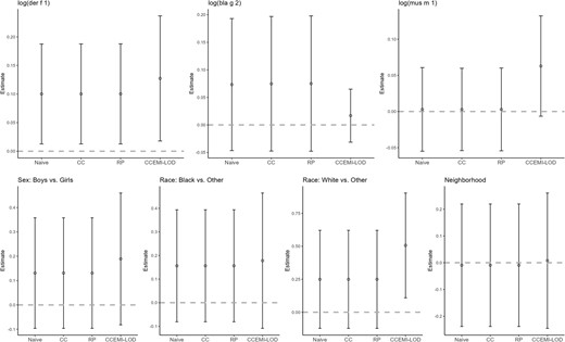
Application to NAAS data: comparison of estimates and 95% CIs of regression coefficients in the linear model of log(FeNO) on indoor allergens using the naive regression, CC, RP, and the CCEMI-LOD methods for handling measurement errors in the indoor allergens.

Open in new tabDownload slide

5 Discussion

Measurement errors are common in environmental epidemiologic research and bias estimates of the effects of environmental exposures. The current literature on the covariate measurement error problem has largely concerned the case of a single exposure. In this article, we propose a constrained CEMI method to correct for measurement errors in more than one environmental exposure in regression analysis. Because most environmental exposures are quantified on a continuous scale, we consider measurement error of continuous exposures. We further extend the constrained CEMI to the settings where exposures are subject to not only measurement error but also LODs.

Our simulations are consistent with previous findings for one X, where CC and RP for incorporating information from an external calibration sample yield biased estimates in the regression setting when the measurement error is nontrivial (Guo and others, 2012). The proposed constrained CEMI method outperforms the alternative methods in eliminating bias in the regression coefficients due to measurement error. The BMI variance estimation yields CIs with coverage rates close to the nominal level. The improvement becomes more pronounced with increased measurement error, covariate effects, or the correlations between covariates. The CCEMI-LOD method performs well even when the proportions of data below LODs are as high as 50%, with close to zero bias and 95% CIs close to the nominal level coverage, when the normality assumption is reasonable for the error-prone measures given the true values of the exposures among those both above and below LODs.

The unconstrained CEMI method implemented using the default settings in the mice package without placing constraints on the imputation matrix performs poorly in the external calibration designs. This highlights the importance of the constraints we impose in the constrained CEMI method and demonstrates that failure to incorporate the strong NDME assumptions in the external calibration settings could cause CEMI to produce unreliable results. The strong NDME assumptions are not required for the interval calibration design.

Rubin’s variance estimation method for MI data, the default method used in the mice package for MI analysis, leads to very wide 95% CIs in the simulations with external calibration. This is not unexpected, as Rubin’s variance estimation method does not apply here because both the calibration and main study data are involved in the imputation but only the main study sample is used in the postimputation analyses. Instead, our BMI variance estimates yield narrower CIs than Rubin’s method with close to nominal level coverage. The BMI method provides consistent variance estimates and CIs with coverage close to nominal level even when the imputation and analysis models are incompatible or misspecified. It requires approximately the same number of bootstraps as bootstrapping complete data and produces consistent variance estimates with just two imputations per bootstrapped sample (von Hippel and Bartlett, 2021).

For the CCEMI-LOD method, we use a tobit regression to impute the error-prone measures below LODs. To ease the computation, we estimate the parameters of the tobit regression using MLEs. The use of MLEs has been discouraged in the MI due to concerns about potentially ignoring some uncertainty. However, von Hippel and Bartlett (2021) showed that the BMI method yields consistent variance estimation whether MLEs or posterior draws are used to create MIs.

We assume the error-prone measures W are independent given the true values X. This may not be true in some settings. When the measurement errors of multiple exposures are correlated, we need to relax our strong NDME assumptions to allow W_j to depend on other ${Wk,k≠j}$ given the true values of the exposures in the imputation model for each W_j, $j=1,…,p$⁠. This is a straightforward extension of the current work.

Previous studies (van Buuren, 2007; Raghunathan and others, 2001; Hughes and others, 2014; Seaman and Hughes, 2016) have stated that the chained equations imputation under a set of linear normal regression models is equivalent to a Gibbs sampler that draws from a multivariate normal distribution if all the other variables are included as predictors and there are no interactions. With the strong NDME assumptions, constraints are imposed on some imputation models, so in the imputation of a variable not all the other variables are included as predictors. These constraints reduce the number of parameters that need to be estimated in both the joint model and conditional models. Under external calibration with all continuous variables and only one X, Guo and others (2012) showed the transformation of the parameters between the joint distribution and the product of conditional and marginal distributions is one-to-one under the multivariate normal with a similar strong NDME assumption, so that the constraints applied to the conditional distributions are transformable one-to-one to become constraints applied to the joint distribution. For example, the independence between W and Y given X in the conditional specification of the model for W is equivalent to specifying the covariance between W and Y to be 0 given X. Therefore, the chained equations imputation is still equivalent to a joint model that draws from a multivariate normal distribution even in the presence of the constraints implied by the strong NDME assumptions. Compared to the joint model approach, the CEMI is potentially more robust because it allows for more flexible conditional models, such as models involving nonlinear link functions, nonlinear relationships with predictors and interactions. Such models are often not compatible with a joint model formulation (Seaman and Hughes, 2018).

The constrained CEMI method offers two advantages over the alternative methods for handling measurement error. First, the constrained CEMI allows the imputation of not only X but also nondetects in W and any missing values in Y or Z in the main study sample. Although we assume Y and Z are fully observed in the main study sample, the same imputation matrices, as shown in Figure 2, can be applied without any modification when Y or Z are incomplete. Thus measurement error, LODs, and missing data can all be handled simultaneously. Second, the constrained CEMI is very flexible and can be applied to more complicated models by modifying the imputation models. For example, a random forest method can be used for imputation using the mice package and a modified chained equations imputation approach can be carried out using the smcfcs package in R to ensure that the imputation and analysis models are compatible (Bartlett and others, 2015).

The constrained CEMI method can be easily implemented using the mice package in R with a user-defined imputation matrix, as shown in Figure 2. By assuming the strong NDME assumptions, constraints are imposed on the imputation matrix. Although the mice package does not include an option for fitting the tobit regression, we have derived a custom tobit function that can be integrated with the mice package. Finally, the BMI for variance estimation can be implemented using the bootImpute package together with the mice package in R. We provide sample codes for implementing our methods in the GitHub https://github.com/yy3019/CCEMI.

Supplementary material

Supplementary material is available at http://biostatistics.oxfordjournals.org

Conflict of interest: None declared.

Funding

The National Institutes of Health (R21ES029668).

Acknowledgments

We thank the Editor, the Associate Editor and the referee for their thoughtful and constructive comments which greatly improved the article.

References