


Summary
The problem of associating data from multiple sources and predicting an outcome simultaneously is an important one in modern biomedical research. It has potential to identify multidimensional array of variables predictive of a clinical outcome and to enhance our understanding of the pathobiology of complex diseases. Incorporating functional knowledge in association and prediction models can reveal pathways contributing to disease risk. We propose Bayesian hierarchical integrative analysis models that associate multiple omics data, predict a clinical outcome, allow for prior functional information, and can accommodate clinical covariates. The models, motivated by available data and the need for exploring other risk factors of atherosclerotic cardiovascular disease (ASCVD), are used for integrative analysis of clinical, demographic, and genomics data to identify genetic variants, genes, and gene pathways likely contributing to 10-year ASCVD risk in healthy adults. Our findings revealed several genetic variants, genes, and gene pathways that are highly associated with ASCVD risk, with some already implicated in cardiovascular disease (CVD) risk. Extensive simulations demonstrate the merit of joint association and prediction models over two-stage methods: association followed by prediction.
1. Introduction
Many complex diseases including cardiovascular diseases (CVD) and atherosclerotic CVD (ASCVD) are multifactorial and are caused by a combination of genetic, biological, and environmental factors. Several research applications and methods continue to demonstrate that a better understanding of the pathobiology of complex diseases necessitates analysis techniques that go beyond the use of established traditional factors to one that integrate clinical and demographic data with molecular and/or functional data. It is also recognized that leveraging existing sources of biological information including gene pathways can guide the selection of clinically meaningful biomarkers and reveals pathways associated with disease risk.
In this article, we build models for associating multiple omics data (e.g., genetics, gene expression) and simultaneously predicting a clinical outcome while considering prior functional information and other covariates. The models are motivated by, and are used for, the integrative analysis of multiomics and clinical data from the Emory Predictive Health Institute, where the goal is to identify genetic variants, genes, and gene pathways potentially contributing to 10-year atherosclerosis disease risk in healthy adults.
Our approach builds and extends recent research on joint integrative analysis and prediction/classification methods developed from the frequentist perspective to the Bayesian setup (Luo and others, 2016; Safo and others, 2021). Unlike two step approaches—integrative analysis followed by prediction or classification—these joint methods link the problem of assessing associations between multiple omics data to the problem of predicting or classifying a clinical outcome. The goal is then to identify linear combinations of variables from each omics data that are associated and are also predictive of a clinical outcome. For instance, the authors in Luo and others (2016) and, Safo and others (2021) combined canonical correlation analysis (CCA) with classification or regression methods for the purpose of predicting a binary or continuous response. Safo and others (2021) proposed a joint association and classification method that combines CCA and linear discriminant analysis and uses the normalized Laplacian of a graph to smooth the rows of the discriminant vectors from each omics data. These joint association and prediction methods have largely been developed from a frequentist perspective. There exist Bayesian factor analysis or CCA methods to integrate multiple omics data (Mo and others, 2018; Klami and others, 2013), but none of these methods have been developed for joint association and prediction of multiple data types. We recognize that there exists Bayesian methods for integrating omics data and predicting a clinical outcome (e.g., survival time) (Wang and others, 2012; Chekouo and others, 2015; Chekouo and others, 2017). However, these methods do not explicitly model the factors that are shared or common to multiple omics and clinical data, and that likely drive the variation in the clinical response.
We make three main contributions to existing Bayesian methods for integrative analysis. First, we consider a factor analysis approach to integrate multiple data types, similar to the methods in ( Shen and others, 2009, 2013; Klami and others, 2013), but we formulate a Bayesian hierarchical model with the flexibility to incorporate other functional information through prior distributions. Our approach uses ideas from Bayesian sparse group selection to identify simultaneously active components and important features within components using two nested layers of binary latent indicators. Importantly, our approach is more general; we are able to account for active shared components as well as individual latent components for each data type. Second, we incorporate in a unified procedure, a clinical response that is associated with the shared components; this allows us to evaluate the predictive performance of the shared components. In addition, our formulation makes it easy to include other covariates without enforcing sparsity on their corresponding coefficients. Including other available covariates may inform the estimation of the shared components, which in turn can result in better predictive performance of the shared components. Third, unlike most integrative methods that use factor analysis, our prior distributions can be extended to incorporate external grouping information. We are able to determine most important groups of features that are associated with important components. Incorporating prior knowledge about grouping information has the potential to identify functionally meaningful variables (or network of variables) within each data type and can improve prediction performance of the response variable.
1.1. Motivating application
There is an increased interest in identifying “nontraditional” risk factors (e.g., genes, genetic variants) that can predict CVD and ASCVD. This is partly so because CVD has become one of the costliest chronic diseases and continues to be the leading cause of death in the U.S. (AHA, 2016). It is projected that nearly half of the U.S. population will have some form of cardiovascular diseases by 2035 and will cost the economy about |$\$2$| billion/day in medical costs (AHA, 2016). There have been significant efforts in understanding the risk factors associated with ASCVD, but research suggests that the environmental risk factors for ASCVD (e.g., age, gender, hypertension) account for only half of all cases of ASCVD (Bartels and others, 2012). Finding other risk factors of ASCVD and CVD unexplained by traditional risk factors is important and potentially can serve as targets for treatment.
We integrate gene expression, genomics, and/or clinical data from the Emory University and Georgia Tech Predictive Health Institute (PHI) study to identify potential biomarkers contributing to 10-year ASCVD risk among healthy patients. The PHI study, which began in 2005, is a longitudinal study of healthy employees of Emory University and Georgia Tech aimed at collecting health factors that could be used to recognize, maintain, and optimize health rather than to treat disease. The goal of the PHI, the need to identify other biomarkers of atherosclerotic cardiovascular diseases, and the data available from the PHI (multiomics, clinical, demographic data), motivate our development of Bayesian methods for associating multiple omics data and simultaneously predicting a clinical outcome while accommodating prior functional information and clinical covariates.
The rest of the article is organized as follows. In Section 2, we present the formulation of the model. In Section 3, we describe our MCMC algorithm and we present how to evaluate our prediction performance. In Section 4, we evaluate and compare our methodology using simulated data. In Section 5, we apply the proposed method to our motivating data. Finally, we conclude our manuscript in Section 6.
2. Model formulation
Our primary goal is to define an integrative approach that combines multiple data types and incorporates clinical covariates, a response variable, and external grouping information. In Section 2.1, we introduce the factor analysis model that relates the different data types. We then adopt a Bayesian variable selection technique in Section 2.2 to select active components and their corresponding important features. We extend the approach to incorporate grouping information in Section 2.3.
2.1. Factor analysis model for integrating multiple data types and clinical outcome
2.2. Bayesian variable selection using latent binary variables
Thus, if the |$j$|th variable in the active |$l$|th component is selected, then the prior of |$a^{(m)}_{lj}$| is a normal distribution with zero mean and variance |$(\tau_{lj}^{(m)})^2\sigma_j^{2(m)}$|. Otherwise, the coefficient |$a^{(m)}_{lj}$| is equal to 0. The prior distribution of the residual variance |$\sigma_j^{2(m)}$| is an inverse Gamma distribution, |$\sigma_j^{2(m)}\sim IG(a_0, b_0)$|. Finally, we assume that |$\gamma^{(m)}_{l}\sim \text{Bernouilli}(q^{(m)})$| and |$q^{(m)}$| follows a Beta distribution |$Beta(a,b)$|.
Our method encompasses three different scenarios: (i) each component is shared across all data types (including the response) that is, |$\gamma^{(m)}_{l}=1$| for every |$m=0,1,\ldots,M,M+1$| and |$l=1,...,r$|. This scenario only accounts for the joint variation between the data types and is assumed in standard CCA methods for high dimensional data integration such as Luo and others (2016) and Safo and others (2018); (ii) none of the |$r$| components is shared across data types, that is, |$\displaystyle \bigcap^{M}_{m=0} \{l=1,...,r;\gamma^{(m)}_{l}=1\}=\varnothing$|. This scenario would be similar to the standard factor analysis for each data type independently and accounts only for the individual variations explained for each data type, and (iii) some components are only shared across the data types. Hence, our method can capture the amount of joint and individual structure of the data types. Our method then encompasses Bayesian CCA and Joint and Individual variation explained (JIVE) methods introduced respectively by Klami and others (2013) and Lock and others (2013). For instance, assume we have two other data types (besides response and clinical covariates), |$r=4$| components, the first two components are shared (i.e., |$\gamma^{(m)}_{1}= \gamma^{(m)}_{2}=1$|, for every |$m$|) and, components 3 and 4 are only associated respectively with data types 1 and 2 (i.e., |$\gamma^{(1)}_{3}=\gamma^{(2)}_{4}=1$| and |$\gamma^{(2)}_{3}=\gamma^{(1)}_{4}=0$|). The models for data types 1 and 2 can then be written as |$\boldsymbol{X}^{(1)}=\boldsymbol{U}\boldsymbol{A}^{(1)}+\boldsymbol{E}^{(1)}=\boldsymbol{U}_{1,2}\boldsymbol{A}_{1,2}^{(1)}+\boldsymbol{U}_{3}\boldsymbol{A}_{3}^{(1)}+\boldsymbol{E}^{(1)}$| and |$\boldsymbol{X}^{(2)}=\boldsymbol{U}\boldsymbol{A}^{(2)}+\boldsymbol{E}^{(2)}=\boldsymbol{U}_{1,2}\boldsymbol{A}_{1,2}^{(2)}+\boldsymbol{U}_{4}\boldsymbol{A}_{4}^{(2)}+\boldsymbol{E}^{(2)}$|, where |$\boldsymbol{U}_{1,2}=(\boldsymbol{U}_{1},\boldsymbol{U}_{2})$| (respectively |$\boldsymbol{A}_{1,2}$|) is the matrix of the first two components of |$\boldsymbol{U}=(\boldsymbol{U}_{1},\boldsymbol{U}_{2},\boldsymbol{U}_{3},\boldsymbol{U}_{4})$| (respectively |$\boldsymbol{A}$|). In this example, |$\boldsymbol{U}_{1,2}$| is the shared component, and |$\boldsymbol{U}_{3}$| and |$\boldsymbol{U}_{4}$| can be considered as the individual latent structures for data types 2 and 3, respectively. Refer to simulations in Section 4 in the main and Section C of the Supplementary materials available at Biostatistics online, respectively for illustrations.
2.3. Incorporating grouping information through prior distributions
In this section, we present how we incorporate known group structures of the |$M$| data types through prior distributions. For that, we introduce a design/loading matrix |$\boldsymbol{P}^{(m)}=(\kappa^{(m)}_{jk})_{ (p_m\times K_m )}$| consisting of |$K_m$| columns of dummy variables coding for group membership, for every |$m=1,...,M$|. More specifically, |$\kappa^{(m)}_{jk}=1$| if variable |$j$| from data type |$m$| belongs to group |$k=1,...,K_m$|, and |$0$| otherwise. Here, we assume that this matrix can be retrieved from external databases. For instance, genes can be grouped using KEGG pathway information or other pathway/network information (Qiu, 2013). Similarly, SNPs can be grouped using their corresponding genes.
The parameter |$b^{(m)}_{lk}$| is assumed to be nonnegative in order to reduce the amount of shrinkage attributable to the |$k$|th important group. Hence, higher values |$b^{(m)}_{lk}$| give more evidence for group information by increasing the effect of features belonging to group |$k$| (see Figure SA.1 of the Supplementary materials available at Biostatistics online for an illustration of the prior of a loading). A similar prior construction was considered by Rockova and Lesaffre (2014) to incorporate grouping information in the context of regression models.
We finally assume that the intercept |$b_{l0}^{(m)}$| follows also a Gamma |$\Gamma(\alpha_0,\beta_b)$|. Correlations between significant features within the same group are captured through the prior of the penalty parameter |$\lambda^{(m)}_{lj}$| (see prior (2.4)). An illustration is presented in Section A.2 of the of the Supplementary materials available at Biostatistics online. As we would expect, as |$\beta_b$| increases and/or |$\alpha_b$| decreases, |$\lambda^{(m)}_{lj}$|’s values of features |$j$| within the same group tend to have a stronger correlation, translating to a higher probability to have similar values.
3. Posterior inference and prediction
For posterior inference, our primary interest is in the estimation of the active component and feature selection indicator variables |$\boldsymbol{\gamma}^{(m)}$|, |$\boldsymbol{\eta}^{(m)}$|, and the loadings |$\boldsymbol{A}^{(m)}=(\boldsymbol{a}^{(m)}_{lj})$|. We implement a Markov Chain Monte Carlo (MCMC) algorithm for posterior inference that employs a partially collapsed Gibbs sampling (van Dyk and Park, 2008) to sample the binary matrices and the loadings. In fact, to sample |$\boldsymbol{\gamma}^{(m)}$|, |$\boldsymbol{\eta}^{(m)}$| given the other parameters, we integrate out all the loadings |$\boldsymbol{A}^{(m)}$|, and we use a Metropolis–Hastings step. We then sample the loadings of selected variables (i.e., |$\eta^{(m)}_{lj}=1$|) |$\boldsymbol{A}_{(\eta)}=(\boldsymbol{A}^{(0)}_{(\eta)},...,\boldsymbol{A}^{(M+1)}_{(\eta)})$| from their full conditional distributions. |$\boldsymbol{A}^{(m)}_{(\eta)}$| is the matrix of loadings |$\boldsymbol{A}^{(m)}$| when |$\eta^{(m)}_{lj}=1$|, |$j=1,...,p_m$|. In Section B of the Supplementary materials available at Biostatistics online, we present a summary of the algorithm and the conditional distributions used to update all the parameters.
For both simulations and observed data analysis, we set the hyperparameters as explained in Section B.6 of the Supplementary materials available at Biostatistics online. In particular, we set |$r=4$| as the maximum number of active components. A larger number can be set as our approach is able to select active components for each data type through the component indicators |$\boldsymbol{\gamma^{(m)}}$|. The choice of |$r=4$| was guided by plotting the eigenvalues against the potential number of components (see Figure C.1 of the Supplementary materials available at Biostatistics online). We observe that the absolute change in the eigenvalues after |$r=4$| was not large, and that the eigenvalues seemed to be leveling off around |$r=4$|. For practical purposes, we recommend users to obtain similar graphs to inform the choice for |$r$|. Further, since our algorithm can determine the component that is associated with each data type (clinical covariates and outcome included), it is likely that different components will be associated with each data type. As such, we recommend that |$r$| should not be less than the number of data types, to allow for different component to be associated with each data type. Sensitivity analysis of the choice of |$r$| and other parameters are shown in Section C.4 of the Supplementary materials available at Biostatistics online.
For both simulated and observed data, we used 65 000 MCMC iterations, with 15 000 iterations as burn-in. To assess the MCMC convergence of our approach, we fitted four MCMC chains with different starting points. As is commonly done in Bayesian variable selection (Chekouo and others, 2015, 2017; Chekouo and others, 2020; Stingo and others, 2011), we assessed the agreement (in particular for binary variables) of the results among the four chains by evaluating the correlation coefficients between the marginal posterior probabilities for feature selection and group selection. These indicated good concordance between the four chains, with all correlations |$>0.97$| for each data type (see Figures G.1 and G.2 of the Supplementary materials available at Biostatistics online). Additional MCMC diagnostics are available in Section G of the Supplementary materials available at Biostatistics online.
3.1. Prediction
Given a model |$\{\boldsymbol{\gamma}^{(m)}$|, |$\boldsymbol{\eta}^{(m)},m=0,1,...,M+1\}$|, we estimate the loadings |$\boldsymbol{A}$| for |$m=0,1,...,M+1$| as |$\hat{\boldsymbol{a}}_{\cdot j (\eta)}^{(m)}=\hat{\sigma}^{2(m)}_j(\bar{\boldsymbol{U}}^T_{(\gamma)}\bar{\boldsymbol{U}}_{(\gamma)}+I_{n_{\gamma}})^{-1}\bar{\boldsymbol{U}}^T_{(\gamma)}\boldsymbol{x}_{\cdot j}^{(m)}$|, the posterior mode of |$\boldsymbol{A}_{(\eta)}$|, where |$\hat{\sigma}^{2(m)}_j$| and |$\bar{\boldsymbol{U}}_{(\gamma)}$| are the means of the values sampled in the course of the MCMC algorithm. Let |$\boldsymbol{X}^{(m)}_{\text{new}}$|, |$m=1,...,M+1$| be the vector of features of a new individual. The latent value |$\boldsymbol{U}$| of a new individual for a given model |$\{\boldsymbol{\gamma}^{(m)}$|, |$\boldsymbol{\eta}^{(m)},m=1,...,M+1\}$|, is estimated as |$\hat{\boldsymbol{U}}_{\text{new},(\gamma)}=(\boldsymbol{\hat{A}}_{(\eta)}D(\boldsymbol{\hat{\sigma}}^{-2})\boldsymbol{\hat{A}}_{(\eta)}^T+I_r)^{\text{-}1}\boldsymbol{\hat{A}}_{(\eta)}D(\boldsymbol{\hat{\sigma}}^{-2})\boldsymbol{x}_{\text{new}\cdot}$|, where |$\boldsymbol{x}_{\text{new}\cdot}=(\boldsymbol{x}^{(1)}_{\text{new}\cdot},...,\boldsymbol{x}^{(M)}_{\text{new},\cdot},\boldsymbol{x}^{(M+1)}_{\text{new},\cdot})$|, |$D(\boldsymbol{\hat{\sigma}}^{-2})$| is the diagonal matrix with elements |$\{\hat{\sigma}^{2(m)}_j,m=1,..,M+1,j=1,...,p_m \}$| on the diagonal, and |$\boldsymbol{\hat{A}}_{(\eta)}=(\boldsymbol{\hat{A}}_{(\eta)}^{(1)},...,\boldsymbol{\hat{A}}_{(\eta)}^{(M)},\boldsymbol{\hat{A}}_{(\eta)}^{(M+1)})$|. Hence, the predictive response is computed as |$\hat{y}_{\text{new}}=\hat{\alpha}_0+\sum_{\boldsymbol{N},\boldsymbol{\gamma}}\hat{\boldsymbol{U}}_{\text{new},(\gamma)}\boldsymbol{\hat{A}}^{(0)}_{(\eta)}p(\boldsymbol{\gamma},\boldsymbol{N}|\bar{\boldsymbol{U}}_{(\gamma)},\boldsymbol{X})$| using a Bayesian model averaging approach (Hoeting and others, 1999) and, where |$\hat{\alpha}_0$| is the posterior mean of the intercept |$\alpha_0$|.
4. Simulation studies
We consider three main scenarios to assess the performance of the proposed methods. In each scenario, there are two data types |$\boldsymbol{X}^{(1)} \in \Re^{n \times p_1}$| and |$\boldsymbol{X}^{(2)} \in \Re^{n \times p_2}$| simulated according to (1), and a single continuous response |$\boldsymbol{y} \in \Re^{n \times 1}$|. We simulate each scenario to have |$r=4$| latent components. The scenarios differ by how many components are shared across data types. In the first scenario, the four latent components are shared across all two data types. The first two shared components affect the response. In the second scenario, none of the |$r$| components is shared across the two data types. Components 1 and 2 are unique to data type 1, and components 3 and 4 are unique to data type 2. Components 1 and 3 are associated with the response in this scenario. In the third scenario, two of the components (1 and 2) are shared, component 3 is unique to data type 1, and component 4 is unique to data type 2. The response is associated with components 1, 3, 4. The second and third scenarios and part of scenario one are found in the web Supplementary materials available at Biostatistics online (see Section C of the Supplementary materials available at Biostatistics online). In each scenario, we generate 20 Monte Carlo data sets for each data type.
4.1. Scenario One: Each component is shared across all data types
This Scenario is assumed in standard CCA methods for high-dimensional data integration. We simulate two data types |$(\boldsymbol{X}^{(1)},\boldsymbol{X}^{(2)})$|, |$\boldsymbol{X}^{(1)} \in \Re^{n \times p_1}$|, and |$\boldsymbol{X}^{(2)} \in \Re^{n \times p_2}$|, |$(n,p_1,p_2)=(200, 500, 500)$| according to (2.1) as follows. Without loss of generality, we let the first |$100$| variables form the networks or signal groups in |$\boldsymbol{X}^{(1)}$| and |$\boldsymbol{X}^{(2)}$|. Within each data type there are |$10$| main variables, each connected to |$9$| variables. The resulting network has |$100$| variables and edges, and |$p_1-100$| and |$p_2-100$| singletons in |$\boldsymbol{X}^{(1)}$| and |$\boldsymbol{X}^{(2)}$|, respectively. The network structure in each data type is captured by the covariance matrices
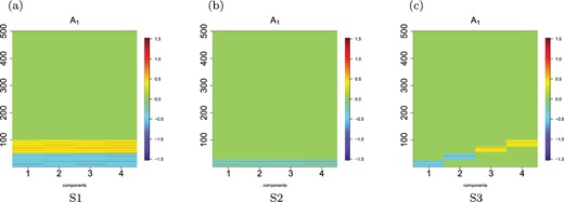
Loadings |$\boldsymbol{A}^{(1)}$| for settings 1, 2, and 3. (a) S1, (b) S2, and (c) S3.
Setting 2: Some variables and some groups in |$\boldsymbol{A}^{(1)} $| and |$\boldsymbol{A}^{(2)}$| contribute to correlation between |$\boldsymbol{X}^{(1)},\boldsymbol{X}^{(2)}$|. In this setting, we let only some variables within the first three signal groups contribute to the association between |$\boldsymbol{X}^{(1)}$| and |$\boldsymbol{X}^{(2)}$|. We generate the entries of |$\boldsymbol{A}^{(1)} \in \Re^{r \times 30}$| and |$\boldsymbol{A}^{(2)} \in \Re^{r \times 30}$| following Setting 1 but we randomly set at most five coefficients within each group to zero.
Setting 3: No overlapping components and all 100 variables contribute to correlation between |$\boldsymbol{X}^{(1)}$| and |$\boldsymbol{X}^{(2)}$|. In Settings 1, 2 (main text) and Settings 4 and 5 of the Supplementary materials available at Biostatistics online, we considered situations where latent components overlapped with respect to the significant variables. In this Setting, there is no overlaps between the latent components. Specifically, data are generated according to Setting 1, but the first 25 signal variables are loaded on component 1, the next 25 variables on component 2, and so on. The last 25 signal variables are loaded on component 4. Similar to Setting 1, there are 10 groups or networks comprising of the 100 signal variables. The 25 variables for each latent component include variables from only 3 signal groups, and distributed as |$40\%$|, |$40\%$|, and |$20\%,$| respectively. This Setting tests our methods ability to identify all 4 components, all 10 groups, and all 100 important variables.
4.1.1. Competing methods
We compare the performance of our methods with association only and joint association and prediction methods. For the association only-based methods, we consider the sparse CCA [SELPCCA] (Safo and others (2018)) and Fused sparse CCA [FusedCCA] (Safo and others (2018)) methods. FusedCCA incorporates prior structural information in sparse CCA by allowing variables that are connected to be selected or neglected together. We perform FusedCCA and SELPCCA using the Matlab code the authors provide. For FusedCCA, we assume that variables within each group are all connected since the method takes as input the connections between variables. For the joint association and prediction methods, we consider the CCA regression (CCAReg) method by Luo and others (2016). We implement CCA regression using the R package CVR. Once all the canonical variates are extracted, they are used to fit a predictive model for the response |$\boldsymbol{y}$|, and then to compute test mean square error (MSE).
4.1.2. Evaluation criteria
To evaluate the effectiveness of the methods, we fit the models using the training data and then compare different methods based on their performance in feature selection and prediction on an independently generated test data of the same size. To evaluate feature selection, we use the number of predictors in the true active set that are not selected (false negatives), the number of noise predictors that are selected (false positives), and F-score (harmonic mean). To evaluate prediction, we use the MSE obtained from the testing set. We use 20 Monte Carlo data sets and report averages and standard errors.
4.1.3. Simulation results
In Table 1, we report averages of the evaluation measures for Scenario One. We first compare our method with incorporation of network information (BIPNet) and without using the network information (BIP). In Settings 1, 2, 4, and 5 (see Table C.1 of the Supplementary materials available at Biostatistics online for Settings 4 and 5), both methods identify one component as important and related to the response. This is not surprising since all 100 important variables on each component overlap in this setting, resulting in our method identifying only one of these components. In Setting 3 where important variables did not overlap on the four latent components, the proposed methods identify at least two components 13 times out of 20 simulated data sets. We note that in general, compared to BIP, BIPNet has lower false negatives, lower false positive rates, competitive or higher harmonic means, and lower MSEs. These results demonstrate the benefit of incorporating group information in feature selection and prediction. We observe a suboptimal performance for both BIPNet and BIP in Settings 2 and 3, more so in Setting 3 where important variables do not overlap on the latent components. We also assess the group selection performance of BIPNet as follows. We compute AUC by using marginal posterior probabilities of group membership |$r_{lk}$|’s. Table C.4 of the Supplementary materials available at Biostatistics online shows that most of groups in Settings 1, 2, and 3 had been identified correctly. However, the method had difficulties selecting groups in cases where only a few features contribute to the association between data types (Settings 2 and 5).
Simulation results for Scenario One (Settings 1–3): variable selection and prediction performances. FNR1; false negative rate for |$\boldsymbol{X}^1$|. Similar for FNR2. FPR1; false positive rate for |$\boldsymbol{X}^1$|. Similar for FPR2; F11 is F-measure for |$\boldsymbol{X}^1$|. Similar for F12; MSE is mean square error.
| Method | Setting. | FNR1 | FNR2 | FPR1 | FPR2 | F11 | F12 | MSE |
|---|---|---|---|---|---|---|---|---|
| BIPnet | S1 | 0.00 (0.00) | 0.00 (0.00) | 0.02 (0.02) | 0.00 (0.00) | 100.00 (0.00) | 100.00 (0.00) | 2.09 (0.04) |
| BIP | S1 | 0.00 (0.00) | 0.00 (0.00) | 0.14 (0.06) | 0.16 (0.04) | 99.73 (0.12) | 99.68 (0.08) | 2.16 (0.04) |
| SELPCCA | S1 | 0.00 (0.00) | 0.00 (0.00) | 0.40 (0.09) | 0.50 (0.12) | 99.21 (0.17) | 99.02 (0.23) | 2.11 (0.04) |
| CCAReg | S1 | 90.25 (1.73) | 90.40 (1.87) | 1.81 (3.32) | 1.71 (3.35) | 15.34 (1.87) | 14.98 (2.01) | 2.01 (0.05) |
| FusedCCA | S1 | 0.00 (0.00) | 0.00 (0.00) | 7.88 (0.76) | 10.40 (0.78) | 86.69 (1.17) | 83.05 (1.08) | 2.14 (0.04) |
| BIPnet | S2 | 0.00 (0.00) | 0.00 (0.00) | 2.81 (0.28) | 3.07 (0.34) | 74.73 (1.9) | 73.34 (2.26) | 2.24 (0.05) |
| BIP | S2 | 0.00 (0.00) | 0.00 (0.00) | 1.82 (0.34) | 1.99 (0.36) | 83.12 (2.82) | 81.91 (2.92) | 2.27 (0.04) |
| SELPCCA | S2 | 51.32 (9.50) | 42.89 (9.42) | 0.10 (0.10) | 0.00 (0.00) | 54.36 (8.08) | 63.42 (8.15) | 2.16 (0.04) |
| CCAReg | S2 | 77.63 (1.87) | 78.68 (1.85) | 3.12 (0.68) | 2.71 (0.67) | 22.80 (1.15) | 23.49 (1.43) | 2.01 (0.05) |
| FusedCCA | S2 | 0.00 (0.00) | 0.00 (0.00) | 19.51 (2.22) | 19.64 (2.53) | 30.39 (1.03) | 30.55 (1.07) | 2.58 (0.06) |
| BIPnet | S3 | 61.05 (2.82) | 59.75 (3.12) | 0.05 (0.03) | 0.00 (0.00) | 54.91 (2.78) | 56.12 (3.03) | 2.35 (0.21) |
| BIP | S3 | 63.00 (2.65) | 60.35 (2.48) | 0.04 (0.03) | 0.06 (0.03) | 52.89 (2.9) | 55.79 (2.63) | 2.64 (0.22) |
| SELPCCA | S3 | 93.40(1.55) | 93.30(1.85) | 0.06(0.06) | 0.00 (0.00) | 11.60 (2.52) | 11.57 (3.00) | 2.72 (0.13) |
| CCAReg | S3 | 88.85 (1.81) | 87.95 (1.89) | 1.44 (0.52) | 1.40(0.50) | 19.83 (2.30) | 21.51 (2.44) | 2.26 (0.14) |
| FusedCCA | S3 | 0.00 (0.00) | 0.00 (0.00) | 3.47 (0.81) | 2.31 (0.55) | 93.89 (1.37) | 95.77 (0.97) | 2.72 (0.11) |
We next compare the proposed methods to other existing methods. For the other methods, we estimate both the first and the first four canonical variates. We report the results from the first canonical variates here, and the results for the first four canonical covariates in Section C, Table C.1 of the Supplementary materials available at Biostatistics online. For feature selection, a variable is deemed selected if it has at least one nonzero coefficient in any of the four estimated components. We observed that for SELPCCA, CCAReg, and FusedCCA in general, the first canonical variates from each data type result in lower false negatives, lower false positives, higher harmonic means, and competitive MSE for Settings 1, 2, 4, and 5 compared to results from the first four canonical variates (see Section C of the Supplementary materials available at Biostatistics online). In Setting 3 where signal variables do not overlap on the four true latent components, we expect the first four canonical variates to have better feature selection and prediction results, and that is what we observe in Table 1. Across Settings 1, 2, 4, and 5, BIP and BIPNet had lower false negatives, lower or comparable false positives, higher harmonic means, and competitive MSEs when compared to two step methods: association followed by prediction. The feature selection performance of the proposed methods was also better when compared to CCAReg, a joint association and prediction method. CCAReg had lower MSEs in general when compared to the proposed and the other methods. BIPNet and BIP had higher false negatives in Setting 3 compared to other Settings, nevertheless lower than CCAReg and SELPCCA. We performed additional simulation studies to investigate the robustness of our BIPnet model to miss specification of our network information as biological networks are often noisy (see Section F.2 of the Supplementary materials available at Biostatistics online). The perturbation of the true network has a slight negative impact on both selection and prediction performances. Nevertheless, prediction and variable selection estimates from using partial information are sometimes better than methods that do not use any network information.
These simulation results suggest that incorporating group information in joint association and prediction methods result in better performance. Although the performance of the proposed methods are superior to existing methods in most Settings, our findings suggest that the proposed methods tend to be better at selecting most of the true signals in the settings where latent components overlap with regards to important variables. In nonoverlapping settings, our methods tend to select some of the true signals (resulting in higher false negatives). However, the proposed methods tend to have lower false positives, which suggest that we are better at not selecting noise variables. This feature is especially appealing for high-dimensional data problems where there tend to be more noise variables.
5. Application to atherosclerosis cardiovascular disease
We apply the proposed methods to analyze gene expression, genetics, and clinical data from the PHI study. The main goals of our analyses are to: (i) identify genetic variants, genes, and gene pathways that are potentially predictive of 10-year atherosclerotic cardiovascular disease (ASCVD) and (ii) illustrate the use of the shared components or scores in discriminating subjects at high- vs low-risk for developing ASCVD in 10 years. There were 340 patients with gene expression and SNP data, as well as clinical covariates to calculate their ASCVD score. The following clinical covariates were added as a third data set: age, gender, BMI, systolic blood pressure, low-density lipoprotein (LDL), and triglycerides. The gene expression and SNP data were each standardized to have mean zero and standard deviation one for each feature. Details for data preprocessing and filtering are provided in Section E.1 of the Supplementary materials available at Biostatistics online.
To obtain the group structure of genes, we performed a network analysis using Ingenuity Pathway Analysis (IPA), a software program which can analyze the gene expression patterns using a built-in scientific literature based database (according to IPA Ingenuity Web Site, www.ingenuity.com). By mapping our set of genes with the IPA gene set, we identified |$p_1=561$| genes within |$K_1= 25$| gene networks. To obtain the group structure of SNPs (|$p_2=413$| SNPs), we identified genes nearby SNPs on the genome using the R package bioMart. We found in total |$K_2=31$| genes that will represent groups for the SNP data. The list of those groups for both data types are shown in Section C of the Supplementary materials available at Biostatistics online.
We divided each of the data type into training (|$n=272$|) and testing (|$n=68$|), ran the analyses on the training data to estimate the latent scores (shared components) and loading matrices for each data type, and predicted the test outcome using the testing data. For the other methods, the training data were used to identify the optimal tuning parameters and to estimate the loading matrices. We then computed the training and test scores using the combined scores from both the gene expression and SNP data. We fit a linear regression model using the scores from the training data, predicted the test outcome using the test scores, and computed test MSE.
To reduce the variability in our findings due to the random split of the data, we also obtained twenty random splits, repeated the above process, and computed average test MSE and variables selected. We further attempted to assess the stability of the variables selected by considering variables that were selected at least 12 times (60%) out of the twenty random splits.
Prediction error and genes and genetic variants selected: For the purpose of illustrating the benefit of including covariates, we also considered these additional models: (i) our BIPnet model, using both molecular data and clinical data (age, gender, Body mass index, Systolic blood pressure, low-density lipoprotein (LDL), triglycerides) [BIPnet+Cov], (ii) our BIP model, using both clinical and molecular data (BIP+ Cov), and (iii) sparse PCA on stacked omics and clinical data (SPCA + Cov). For sparse PCA, we used the method of Witten and others (2009) with |$l_1$|-norm regularization. We were not able to incorporate clinical data in the integrative analysis methods under comparison since they are applicable to two datasets. Figure 2 shows marginal posterior probabilities (MPP) of the four components for each datatype (SNPs, mRNA, and response) for one random split of the data. It shows that for each of the four methods, only one component is active (i.e., MPP|$>0.5$|) for gene expression, and two components for SNP data. None of the component is active for the response variable when applied to methods without clinical data (BIPnet and BIP). However, when applied to methods that incorporate covariates (BiPnet+Cov, BIP+Cov), we can obviously identify at least one active component for the response variable. Note that the MPPs for covariates [Figure (a) and (b)] are 1. This is because we do not select covariates. Our findings show the importance of incorporating clinical data in our approach.
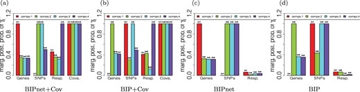
MPPs of the four component indicators, |$\gamma^{(m)}_{l}$|, |$l=1,2,3,4$|, and |$m=$|Response (i.e., ASCVD scores), Genes, SNPs, and covariates, with respect to our four proposed methods. (a) BIPnet+Cov, (b) BIP+Cov, (c) BIPnet, and (d) BIP.
Table 2 gives the average test mean square error and numbers of genes and genetic variants identified by the methods for twenty random split of the data. For FusedCCA, we assumed that all genes within a group are connected (similarly for SNPs). We computed the first and the first four canonical variates for FusedCCA, SELPCCA, and CCAReg using the training data set, and predicted the test ASCVD score using the combined scores from both the gene expression and SNP data. BPINet+ Cov and BIP + Cov have better prediction performances (lower MSEs) when compared to BIPNet, BIP, and the other methods. We also observe that BIPNet and BIPNet + Cov tend to be more stable than BIP and BIP + Cov (125 genes and 55 SNPs vs 0 genes and 54 SNPs selected at least 12 times). Together, these findings demonstrate the merit in combining molecular data, prior biological knowledge, and clinical covariates in integrative analysis and prediction methods.
Average test mean squared error and number of variables selected by the methods for twenty random split of the data. Genes/SNPs selected |$\ge 12$| are genes or snps selected at least 12 times out of twenty random splits. Subscripts 1 and 4 respectively denote results from the first and the first four canonical variates. MSE is mean square error.
| Method | MSE | Average | Average | Genes selected | SNPs selected |
|---|---|---|---|---|---|
| no. of genes | no. of SNPs | |$\ge 12$| times | |$\ge 12$| times | ||
| BIPnet | 1.362 (0.033) | 128.35 | 113.65 | 125 | 55 |
| BIPnet + Cov | 0.758 (0.125) | 122 | 95.8 | 125 | 55 |
| BIP | 1.363 (0.032) | 68.7 | 88.8 | 0 | 54 |
| BIP + Cov | 0.766 (0.153) | 54.7 | 82.5 | 0 | 54 |
| SPCA|$_1$| + Cov | 1.372 (0.034) | 0 | 29.45 | 0 | 29 |
| SPCA|$_4$| + Cov | 1.390 (0.033) | 22.40 | 134.30 | 0 | 113 |
| SELPCCA|$_1$| | 1.366 (0.034) | 56.25 | 29.00 | 1 | 17 |
| SELPCCA|$_4$| | 1.371 (0.037) | 271.450 | 155.45 | 83 | 81 |
| CCAReg|$_1$| | 1.371(0.008) | 48.85 | 43.55 | 0 | 0 |
| CCAReg|$_4$| | 1.385 (0.040) | 20.55 | 24.75 | 0 | 9 |
| FusedCCA|$_1$| | 1.367 (0.032) | 561 | 401.35 | 561 | 400 |
| FusedCCA|$_4$| | 1.383 (0.038) | 561 | 407.60 | 561 | 408 |
We further assessed the biological implications of the groups of genes and SNPs identified by the proposed methods. We selected (MPP |$>$| 0.5) in total 125 genes and 55 SNPs at least 12 times out of the 20 random splits for both BIPNet and BIPNet + Cov (see Figure 2, and Figures E1 and E2 of the Supplementary materials available at Biostatistics online for a random split). Networks 1 and 10 (refer to Table D2 of the Supplementary materials available at Biostatistics online for group description) were identified 18 times (90%) out of the 20 random splits of the data. Networks 1 and 10 both have cancer as a common disease. Research suggest that CVD share some molecular and genetic pathways with cancer (Masoudkabir and others, 2017). In addition, Cell-To-Cell signaling and interaction that characterizes network 10 has led to novel therapeutic strategies in cardiovascular diseases (Shaw and others, 2012). Genes PSMB10 and UQCRQ, and SNPs rs1050152 and rs2631367 were the two top selected genes (highest averaged MPPs) and SNPs respectively across the 20 random splits (see Figures E3 and E4 of the Supplementary materials available at Biostatistics online for a random split). The gene PSMB10, a member of the ubiquitin-proteasome system, is a coding gene that encodes the Proteasome subunit beta type-10 protein in humans. PSMB10 is reported to play an essential role in maintaining cardiac protein homeostasis (Li and others, 2018) with a compromised proteasome likely contributing to the pathogenesis of cardiovascular diseases (Wang and Hill, 2015). The SNPs rs1050152 and rs2631367 found in genes SLC22A4 and SLC22A5, belong to the gene family SLC22A which has been implicated in cardiovascular diseases. Other genes and SNPs with MPP |$> 0.85$|, on average, are reported in Tables C1 and C3 of the Supplementary materials available at Biostatistics online. These could be explored for their potential roles in cardiovascular (including atherosclerosis) disease risk.
Discriminating between high- vs low-risk ASCVD using the shared components: We illustrate the use of the shared components or scores in discriminating subjects at high- vs low-risk for developing ASCVD in 10 years. For this purpose, we dichotomized the response into two categories: low-risk and high-risk patients. ASCVD score less or equal to the median ASCVD was considered low-risk, and ASCVD score above the median ASCVD was considered high-risk. We computed the AUC for response classification using a simple logistic regression model with the most significant (i.e., the highest MPP for our method) component associated with the response as covariates. For the other methods, the AUC was calculated using the first canonical correlation variates from the combined scores. Figure 3 shows that the components selected by our methods applied to the omics and clinical data are able to discriminate clearly the two risk groups compared to our methods applied to the omics data only. The estimated AUCs for the omics plus clinical covariates are much higher than those obtained from omics only applications (e.g., AUC is 1.00 for the training set and AUC is 0.94 for the test set using BIPnet+Cov). When compared to the two-step methods CCAReg and SELPCCA, the estimated AUCs from our methods are considerably higher than the AUC’s from these methods. We applied BIPNet without the assumption that |$\eta_{lj}^{(M+1)}=\gamma_l^{(M+1)}=1$| that is, without assuming that for clinical covariates, all components are active, and all clinical covariates are relevant. Results show that (i) most of the clinical covariates were selected by the model with LDL being the only covariate deemed irrelevant by our model and (ii) there is a common active component between covariates and the response variable which suggests that the clinical covariates are mostly associated with the response. Refer to Section E.1 and Figure E.5 of the Supplementary materials available at Biostatistics online for more details. We also fitted a binomial regression model for ASCVD risk prediction using only clinical data as covariates, and we found an AUC of 0.93 for the test set, which shows for this particular application, SNP and gene expression do not contribute significantly to high AUC values. However, we performed simulation studies that showed the importance of incorporating omics and/or clinical covariates in BIPNet (see Section F.1 of the Supplementary materials available at Biostatistics online).
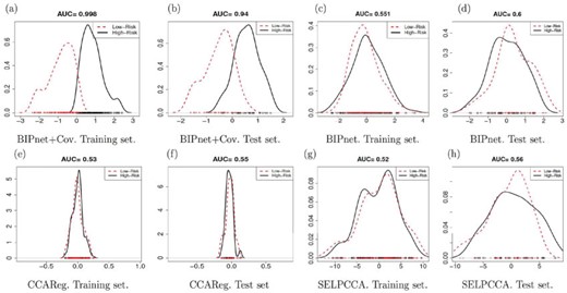
Estimated latent U scores on both training and test sets for low and high CVD risks with respect to our methods and competing methods.
6. Conclusion
We have presented a Bayesian hierarchical modeling framework that integrates in a unified procedure multiomics data, a response variable, and clinical covariates. We also extended the methods to integrate grouping information of features through prior distributions. The numerical experiments described in this manuscript show that our approach outperforms competing methods mostly in terms of variable selection performance. The data analysis demonstrated the merit of integrating omics, clinical covariates, and prior biological knowledge, while simultaneously predicting a clinical outcome. The identification of important genes or SNPs and their corresponding important groups ease the biological interpretation of our findings. Together, these findings demonstrate the importance of onestep methods like we propose here, and also the merit in incorporating both clinical and molecular data in integrative analysis and prediction models.
Several extensions of our model are worth investigating. First, using latent variable formulations, we can naturally extend our approach to other types of response variables such as survival time, binary or multinomial responses or mixed response outcomes (e.g., both continuous and binary). Second, the proposed method is only applicable to complete data and does not allow for missing values. A future project could extend the current methods to the scenario where data are missing using Bayesian imputation methods or the approach proposed by Chekouo and others (2017) for missing blocks of data. Third, we assume that the omics data are continuous. A future method will extend the current work to other omics data types (e.g., binary, categorical or count).
Software
We have created an R package called BIPnet for implementing the methods. It also contains functions used to generate simulated data. Its source R and C codes, along with the user pdf manual are available in the GitHub repository https://github.com/chekouo/BIPnet.
Supplementary material
Supplementary material is available at http://biostatistics.oxfordjournals.org.
Acknowledgments
We are grateful to the Emory Predictive Health Institute for providing us with the gene expression, SNP, and clinical data. Conflict of Interest: None declared.
Funding
National Institutes of Health (NIH) (5KL2TR002492-04 to S.S. in part); and Natural Sciences and Engineering Research Council of Canada (NSERC) Discovery (RGPIN-2019-04810 to T.C., in part).
References
AHA (
Author notes
Thierry Chekouo and Sandra E. Safo contributed equally.
