


Summary
The process of identifying and quantifying metabolites in complex mixtures plays a critical role in metabolomics studies to obtain an informative interpretation of underlying biological processes. Manual approaches are time-consuming and heavily reliant on the knowledge and assessment of nuclear magnetic resonance (NMR) experts. We propose a shifting-corrected regularized regression method, which identifies and quantifies metabolites in a mixture automatically. A detailed algorithm is also proposed to implement the proposed method. Using a novel weight function, the proposed method is able to detect and correct peak shifting errors caused by fluctuations in experimental procedures. Simulation studies show that the proposed method performs better with regard to the identification and quantification of metabolites in a complex mixture. We also demonstrate real data applications of our method using experimental and biological NMR mixtures.
1. Introduction
Over the last several decades, the field of metabolomics has increasingly gained attention among postgenomics technologies (Dieterle and others, 2006) due to its ability to study the state of a biological system at the molecular level. In particular, metabolites are the direct outcomes of all genomic, transcriptomic, and proteomic responses to environmental stimuli, stress, or genetic mutations (Fiehn, 2002). Small changes in metabolite concentration levels might reveal crucial information that is closely related to disease status (Gowda and others, 2008), drug resistance (Thulin and others, 2017), and the biological activity of chemicals derived from diet and/or environment (Daviss, 2005). Therefore, metabolomics has become an increasingly attractive approach for researchers in many scientific areas such as toxicology (Ramirez and others, 2013), food science and nutrition (Wishart, 2008a), and medicine (Putri and others, 2013).
Nuclear magnetic resonance (NMR) spectroscopy is one of the premier analytical platforms to acquire data in metabolomics. It is renowned for the richness of information, rapid and straightforward measurements, high level of reproducibility, and minimal sample preparation (Wishart, 2008b). Each metabolite is uniquely characterized by its own resonance signature, namely |$^1H$| NMR chemical shift fingerprint. Every spectral peak is generated by a distinct hydrogen nucleus resonating at a particular frequency, which is measured in parts per million (ppm) relative to a standard compound (Dona and others, 2016). For a particular metabolite, depending on its chemical structure, one or more peaks can show up at specific locations on the chemical shift axis. At the same time, the height of every spectral peak is directly proportional to the concentration of the corresponding metabolite in the mixture.
As an illustration, Figure 1 shows individual |$^1H$| NMR spectra of three metabolites (Figure 1(a)–(c)) under an ideal experimental condition. In each panel, the x-axis denotes the chemical shift which is measured in ppm while the y-axis represents the relative peak intensity corresponding to each chemical shift. Additionally, whenever a peak is mentioned, it is referred to a small symmetrical segment of the spectrum; and the chemical shift corresponds to the center of the peak is known as a peak location. Ideally, given a mixture spectrum composed of several metabolites as shown in Figure 1(d), one could overlay the figure with each individual reference spectrum such as Figure 1(a)–(c)) to potentially identify each metabolite in the mixture if the signals match. The process of identifying individual metabolites in a complex mixture is called identification. Simultaneously, how much each metabolite contributes to the mixture is quantified by their corresponding peak intensities in the mixture spectrum. The process of estimating the concentration of each metabolite in the mixture is called quantification. Therefore, the NMR fingerprint and corresponding peak intensities are keys to any approaches to identify and quantify metabolites present in complex biological mixtures.
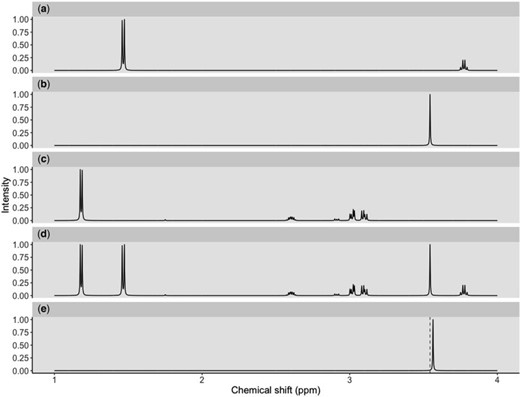
Three reference spectra of L-alanine (a), glycine (b), and 3-aminoisobutanoic acid (c) convolve a mixture spectrum (d) in an ideal condition. Another mixture spectrum (e) has the glycine peak shifted to the right from the referenced location (dashed line).
A conventional approach, which involves manual assignment protocols, has been previously reported (Dona and others, 2016). The manual approach relies on experienced spectroscopists to overlay the observed spectrum with reference spectra of pure compounds to decide which particular metabolites are present in the mixtures, so the whole process is time-consuming, labor-intensive, and prone to biases towards operator knowledge and expectations (Tulpan and others, 2011). Automating the process of metabolite identification and quantification is desired, but there exists two major obstacles. First, uncontrollable sample perturbations are inherent to every metabolomics study, which arise from a variety of sources such as variation in experimental factors (e.g., pH, temperature, and ionic strength), instrument instability, and inconsistency in sample handling and preparation. As a result, NMR signals of a metabolite may deviate from their referenced positions, which, in turn, makes it harder for any matching procedures. Figure 1(e) illustrates such shifting errors in signal positions, where the glycine peak is shifted to the right of its referenced location at 3.54 ppm (i.e., dashed line). Second, the number of candidate metabolites in the database always exceeds the number of actual sources of signals in the spectra, which raises a sparsity issue. For example, the number of metabolites detected from intact serum/plasma is in the range of 30 or less which is far fewer than the 4229 blood metabolites in the Human Serum Metabolome (Psychogios and others, 2011). The combination of the two factors makes the detection and interpretation of metabolite-specific signals challenging in practice.
Regularized regression approaches such as Lasso, elastic net, and adaptive Lasso seem to be intuitive choices to handle the sparsity problem because of their built-in regularization capability. However, they are not capable of addressing peak shifting errors. Recently, high-dimensional regression with measurement errors in covariates is an emerging statistical research area. For example, to deal with the measurement error problem, Sørensen and others (2015) and Datta and Zou (2017) proposed different modifications of Lasso; and Sørensen and others (2018) introduced methods based on the matrix uncertainty selector (Rosenbaum and Tsybakov, 2010). However, these approaches could not be applied to the problem of shifting errors due to two key differences. First, these works assume that the responses and covariates are correctly matched, but the covariates are subject to additive measurement errors. However, in the discussed problem, the observed spectral intensities of a mixture are assumed to be generated from mismatched covariates, i.e., the intensities of compounds with shifting errors. Second, replicates of covariate measurements or an external validation sample are traditionally required to calibrate the models to deal with measurement errors in covariates (Carroll and others, 2006). However, neither of them is available for the type of NMR data being considered. In a different manner, Bayesil (Ravanbakhsh and others, 2015), Chenomx (Chenomx, 2015), and ASICS (Tardivel and others, 2017; Lefort and others, 2019) develop their own methodology to deal with both problems. More precisely, Bayesil partitions the sample spectrum into disjoint regions before applying a probabilistic approach to assign a low probability to an undesirable match and vice versa. Additionally, an automated Profiler module of a popular proprietary software, namely Chenomx, utilizes a linear combination of Lorentzian peak shape models of reference metabolites to reconstruct the observed mixture spectrum (Weljie and others, 2006). Uniquely, ASICS learns warping functions to minimize the difference between the observed and reconstructed spectra before quantifying individual metabolite concentration. However, none of the methods has yet been demonstrated to be a gold standard in practice.
Herein, we introduce a new approach to automatically identify and quantify metabolites in complex biological mixtures. This parsimonious proposed method is shown to be efficient by simultaneously addressing both problems of shifting errors and the sparsity of some abundant metabolites present in mixtures. Specifically, the method first conducts the variable selection to identify correct metabolites in a mixture with nonzero coefficients. Second, the method performs a postselection coefficient estimation to quantify metabolite concentration after correcting for shifting errors using an embedded novel weight function. We demonstrate the effectiveness of the proposed model using simulated data, experimental NMR mixtures, and biological serum samples. Interesting findings are further emphasized when the method is compared with popular regularized regression models including Lasso (Tibshirani, 1996), elastic net (Zou and Hastie, 2005), and adaptive Lasso (Zou, 2006), and other existing fitting models including Bayesil, Chenomx, and ASICS.
2. Model and methodology
2.1. Backgrounds
Each NMR spectrum after being preprocessed by apodization, phasing, and baseline correction can be represented as a pair of equally spaced vector of chemical shifts typically ranging from |$0$| to |$10$| ppm and a same length vector of the corresponding relative intensity of the resonance. Depending on the resolution of the instrument or the spectrum, the total number of features in a spectrum is in the order of |$10^3$|–|$10^4$| (Astle and others, 2012). However, some NMR signals with low intensities might correspond with instrumental noise, which are not reliable for identifying metabolites in a complex mixture. Thus, we define each NMR spectrum of interest as a pair of (|${{{\mathbf x}}, {{\mathbf y}}}$|), where |${{\mathbf y}} = \{y_i\}_{i = 1}^{n}$| are the observed collection of signal intensities such that |$\forall y_i > c_{0}$|, and |${{\mathbf x}} = \{x_{i}\}_{i = 1}^{n}$| are the corresponding chemical shifts. Here, a positive constant |$c_{0}$| serves as a threshold to remove low-intensity signals that are likely to be noise while reducing the number of features to be considered in our model. Details about the selection of |$c_{0}$| are described in Section 4.
2.2. Spectrum model with shifting errors
Models (2.1) and (2.3) imply a mismatch between the observed and referenced intensities (i.e., |$y_i$| and |$y^{\dagger}_i)$| of the mixture. Such shifting deviations need to be corrected to ensure the consistent estimation of |${{\boldsymbol\beta}}$| and accurate identification of the compounds present in the mixture. In Section 2.3, we propose a shifting-corrected regularized regression estimation procedure to correct for the positional errors in the spectral signals.
2.3. Methodology
Here, (2.6) is a constrained regularized optimization, where the non-negativity constraint on |$\beta_j$| is due to the non-negativity of metabolite concentrations in our problem. For general problems without constraints, we may impose the penalty |$\lambda \sum_{j=1}^{p} |\beta_j|$| in (2.6). Note that this optimization problem is more complex than the classical Lasso optimization and may not be convex, since the weights |$w_{ik}$| also depend on the regression coefficients |${{\boldsymbol\beta}}$|.
Compared to (2.4), the loss function |$W({{\boldsymbol\beta}})$| takes into account any potential signal shifting for each location |$x_i$| by including the pairwise distance |$s_{ik}$| corresponding to each element in the search window |$\{\min(1,i-d), \ldots,i,\ldots, \max(i+d, n)\}$|. These pairwise distances are weighted by |$w_{ik}$| such that the large |$s_{ik}$| is multiplied by a small value and vice versa, where the weight |$w_{ik}$| decays exponentially as |$s_{ik}$| increases.
Let |$\hat{{{\boldsymbol\beta}}}$| be a minimizer of (2.6) where |$\hat{{{\boldsymbol\beta}}} = (\hat{\beta}_{1}, \ldots, \hat{\beta}_{p})^{ \mathrm{\scriptscriptstyle T} }$|. Additionally, let |$\mathcal{A} = \{j : j \in \{1,\ldots,p\}, \hat\beta_j > 0\}$| be the active set of the metabolites which are identified as present in the target mixture. We define |$\hat{s}_{ik} = \{ y_i - \hat{\beta}_{0} - \sum_{j \in \mathcal{A}} \hat{\beta}_j g_j(x_k; l_j, r_j) \}^2$|, and |$\hat{w}_{ik} = \phi(\hat{s}_{ik};\sigma_0) \big(\sum_{k=k_l}^{k_u} \phi(\hat{s}_{ik};\sigma_0)\big)^{-1}$|. At each peak location |$x_{i}$| of the mixture, the value |$\arg\max_{k}\{\hat{w}_{ik}\}$| together with the reference peak locations around |$x_{i}$| can be used to estimate and correct for the shifting errors.
The tuning parameter |$\sigma_0$| can be considered as a weight distributor for each search window |$\{\min(1,i-d), \ldots,i,\ldots, \max(i+d, n)\}$| corresponding to |$x_i$|. Smaller |$\sigma_0$| yields a narrower weight distribution, which results in more weights close to 0. In this regard, an extremely small |$\sigma_0$| would assign the weight of 1 to the smallest |$s_{ik}$| while the remaining weights are essentially 0. On the other hand, a large |$\sigma_0$| would flatten out the weight distribution, which in turn loses the ability to detect the signal shifting. Given |$g_j(x_k; {{\mathbf l}}_j ) > 0$||$\forall j,k$|, |$s_{ik}$| takes a value between |$0$| and |$y_i^2$|. In general, we suggest |$\sigma_{0}$| to be between |$\max(y_i^2)/3$| and |$\max(y_i^2)/6$|, |$i = 1, \ldots, n$|, to maintain the smoothness in weight distribution. More discussion about the sensitivity of |$\sigma_0$| on the performance of the proposed method is included in Section 4.
3. Implementation
In this section, we provide the computation algorithms to solve the shifting-corrected regularized estimation (2.6) proposed in Section 2.3.
3.1. Coordinate descent
It is worth noting that if there is no non-negativity constraint on |$\beta_j$| for all |$j$|, and the Lasso penalty |$\lambda \sum_{j=1}^{p} |\beta_j|$| is used in (2.6), the coordinate descent algorithm updates |$\beta_j$| by the soft-thresholding operator as done by Friedman and others (2007).
At each iteration, the algorithm updates each regression coefficient |$\beta_j$| separately, which requires |$O(p)$| computation steps. Meanwhile, there are |$n(2d + 1)$| weights to update for each updated |$\beta_j$|. The total computational complexity is |$O\{np(2d + 1)\}$| per iteration. Additionally, the process of looping through all regression coefficients |$\beta_j$| is iterated until the convergence criterion |$\|\hat{{{\boldsymbol\beta}}}^{(u)} - \hat{{{\boldsymbol\beta}}}^{(u-1)} \| < 10^{-5}$| is met or when the maximum number of iterations, which is set at 1000, is reached. Intuitively, as |$W({{\boldsymbol\beta}})$| is a convex function given the weights |$\{w_{ik}\}$|, the algorithm would converge if the initial weights are close to the ones with the true |${{\boldsymbol\beta}}$|. While |$W({{\boldsymbol\beta}})$| is a nonconvex function of |$\beta$| as |$\{w_{ik}\}$| changes with |$\beta$|, and our proposed algorithm is not guaranteed to converge to a global optimum, we find that the results are not sensitive to the initial values in the simulation studies and the real data analysis. The theoretical convergence properties of the proposed method will be investigated in future work.
Let |${{\mathbf G}}_{n \times p}$| be the reference library data matrix, where the |$j$|th column of |${{\mathbf G}}$| consists of the spectrum |$\{g_j(x_{i};{{\mathbf l}}_j)\}_{i = 1}^{n}$| of the |$j$|th metabolite in (2.2). As before, |${{\mathbf y}}_{n \times 1}$| is the |$n$|-dimensional vector representing the spectrum of the target mixture. Given the penalty parameter |$\lambda$| chosen by the cross-validation (CV) criterion, the tuning parameter |$\sigma_0$| in the weight function (2.5), and the search window size |$d$|, the main steps of the proposed optimization algorithm are outlined below.
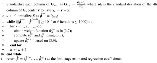
Coordinate descent algorithm to solve |${{\boldsymbol\beta}}$| in (2.6)
3.2. Cross-validation
A decreasing sequence of |$\lambda$| values is used to calculate the corresponding prediction errors through CV. The optimal penalty parameter |$\lambda$| associated with the smallest error is chosen. Similar to Lasso’s pathwise coordinate descent (Friedman and others, 2010), the sequence of |$\lambda$| is generated such that its maximum |$(\lambda_{\max})$| is the minimum penalty value that all the estimated coefficients become 0. Specifically, |$\lambda_{\max}$| is computed as |$\lambda_{\max} \geq \left|\sum_{i=1}^{n}w^*_{ik}y_ig_j(x_k; {{\mathbf l}}_j )\right|$| where |$w^*_{ik} = \frac{\phi(s^*_{ik})}{\sum_k \phi(s^*_{ik})} = \frac{1}{2d + 1}$| with |$s^*_{ik} = y_i^2$|. Then, we define |$\lambda_{\min} = c \lambda_{\max}$| for a small positive value of |$c$|. The |$\lambda$| sequence of length |$M_0$| is constructed by linearly decreasing from |$\lambda_{\max}$| to |$\lambda_{\min}$| on a log scale, where |$c$| and |$M_{0}$| are recommended to be 0.0001 and 50, respectively according to Friedman and others (2010).
The constructed sequence of penalty values |$\lambda$| is then used for 5-fold CV as outlined in Algorithm 2. For both the observed mixture spectrum (response) and the spectra in the reference library (covariates), all NMR signals after thresholding with |$c_0$| are randomly partitioned into five sets. During the random partition, it is almost certain that some signals of each peak are used for training, which is sufficient to detect any peak shifting. Each of the five sets is used for validation while the other four sets are used for training. For a given value of |$\lambda$| in the sequence, the regression coefficients are estimated using the training set. The estimated loss |$W({{\boldsymbol\beta}})$| in (2.6), which is obtained using the estimated coefficients, is evaluated on the validation set. The CV loss corresponding to each |$\lambda$| is the average loss over the five sets; the cross-validated penalty value is chosen as the minimizer of the CV loss. Similarly, we apply the standard 5-fold CV to choose the penalty values for Lasso, elastic net, and adaptive Lasso. The main difference is that the three methods utilize standard least-squares loss while the proposed method uses the weighted loss in (2.6) to account for the shifting errors.
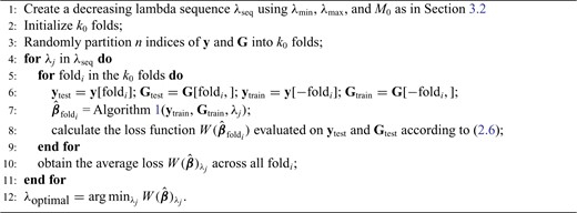
Cross-validation
3.3. Concentration estimation
Here, the non-negativity constraint is again enforced such that |$\tilde{\beta_j} = 0$| for |$j \in \mathcal{A}$| if |$\tilde{\beta_j} < 0$| to ease the interpretation of non-negative metabolite concentration. Additionally, as the concentration estimation |$\tilde{{{\boldsymbol\beta}}}$| in (3.10) is conditional on the selection results, i.e., the estimation of |$\hat{{{\boldsymbol\beta}}}$| in (3.9) as well as the correction for shifting error, the inference for |$\tilde{{{\boldsymbol\beta}}}$| is more complicated than the usual post-selection Lasso estimators. In order to study the impact of the two steps on the least square estimator |$\tilde{{{\boldsymbol\beta}}}$|, one could consider the stability selection procedure, as in Meinshausen and Bühlmann (2010). More discussion about this is described in Section S1.3 of the Supplementary material available at Biostatistics online.
4. Simulation studies
The evaluation criteria used to compare the performance of different methods were accuracy, sensitivity, and specificity. Accuracy was calculated as a ratio of correctly labeled metabolites (true positives plus true negatives) to the total number of metabolites in reference library. Similarly, sensitivity was obtained as a fraction of the correctly identified metabolites (true positives) relative to the total number of true metabolites. Moreover, specificity was measured by dividing the number of unidentified metabolites by the number of metabolites not present in a mixture. The correct or incorrect metabolites in a mixture were determined based on their corresponding postselection error-corrected least squares estimates |$\tilde{{{\boldsymbol\beta}}}$| defined in (3.10). Additionally, Figure S1 of the Supplementary material available at Biostatistics online showed a decline in the loss function as the number of iterations increased. More precisely, the objective function was stabilized within the first 50 iterations across simulated and real mixtures, which verified the convergence of the proposed algorithm in practice.
Two simulation studies were conducted with a reference database of 200 compounds generated directly from (2.2) for chemical shifts ranging from 0.9 to 9.2 ppm with an equal space of 0.001 ppm, excluding the water suppression region between 4.6 and 4.8 ppm. The peak list for each compound |${{\mathbf l}}_j = (l_{j1}, \ldots, l_{jn_j})$| was then randomly selected from the available chemical shifts, with |$n_j$| ranging from 1 to 10. The corresponding peak heights were generated from the uniform distribution |$(0.1,1)$|, which were then used to calculate the multiplier factor |${{\mathbf v}}_j = (v_{j1}, \ldots, v_{jn_j})$| as described in Section 2.2. The shape parameter |$r_j$| was fixed at 0.002 to maintain the sharp shape of an NMR peak. Each resulting spectrum was standardized such that its maximum peak intensity was set to 1. Our simulation studies only consisted of comparisons between the proposed methods and existing regularized regression models (i.e., Lasso, elastic net, and adaptive Lasso) because Bayesil, Chenomx, and ASICS only handled raw |$^1H$| NMR data which were not obtainable through simulation. The performance comparison between the proposed method and existing software including Bayesil, Chenomx, and ASICS, was illustrated in Section 5. Due to limited space, we only reported in detail one of the simulation studies in the main text. The additional simulation study was discussed in Section S2 of the Supplementary material available at Biostatistics online.
A target mixture in the simulation as shown in Figure 2(a) was created by adding three individual spectra with random noise to resemble experimental variations. More specifically, true parameters were set up such that |$\beta_1 = \beta_2 = \beta_3 = 1$|, and |$\beta_j = 0$| for |$j = 4, \ldots, 200$|. Furthermore, positional noise, i.e., peak shifting errors were explicitly examined by purposely shifting locations of chosen peaks. The peak |$M1$| in Figure 2(a) was shifted to the right from its referenced location |$M1_{ref}$| while |$M2$| and |$M3$| stayed unchanged. The amount of chemical shift variation was applied in an increasing fashion, i.e., |$\delta_{11} \sim \mathrm{Unif}(-K, K)$|, such that |$K = \{0.01, 0.02, 0.03, 0.04\}$| ppm respectively to assess the performance of various methods. The whole process of adding random noise to a generated mixture spectrum and shifting peak locations was repeated 200 times. Section S3.2 of the Supplementary material available at Biostatistics online discussed in detail how the proposed method behaved as the variance of the added noise increased. Additionally, based on the sensitivity analysis results (Tables S3–S6 of the Supplementary material available at Biostatistics online), we set |$d$| defined in (2.5) to be the closest integer capturing the maximum shifting variation. In other words, with equal space of 0.001 ppm between chemical shifts, |$d$| was set to be 10, 20, 30, and 40 in correspondence with |$K = \{0.01, 0.02, 0.03, 0.04\}$| ppm, respectively.
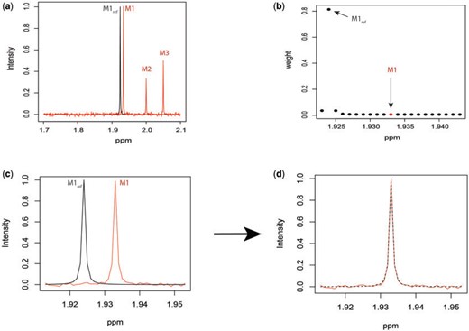
Simulated mixture spectrum (three rightmost peaks) with added random noise (a) overlaid with the reference counterpart |$M1_{\rm ref}$| (leftmost peak) of |$M1$| in the simulation. Weight plot for the shifted peak (b) potentially relocates the shifted peak by detecting the noncentered maximum weight. As a result, shifted peak (c) is corrected to match its referenced peak (d).
Once a mixture was created, a threshold level |$c_0$| defined in Section 2.1 was obtained such that |$c_0$| was greater than |$7\%$| of the area under the mixture spectrum curve (AUC), i.e., |$c_0 = 7\% \mbox{AUC}$| (Ahmed, 2005). An extended simulation study reported in Section S3.1 of the Supplementary material available at Biostatistics online assessed how changing |$c_0$| would affect the performance of the proposed method. We evaluated different values of |$c_0$| (i.e., |$5\%$|, |$7\%$|, |$10\%$|, and |$12\%$||$\mbox{AUC}$|) in conjunction with different |$d$| values (i.e., |$5$|, |$10$|, |$15$|, |$20$|, and |$25$|). Consistent results across |$c_0$| values served as an assurance to continue both simulation studies and real data analysis using |$c_0 = 7\% \mbox{AUC}$|. Furthermore, a joint analysis for various values of both |$\sigma_0$| and |$d$| defined in (2.5) was summarized in Section S3.1 of the Supplementary material available at Biostatistics online. The results confirmed the choice of |$\sigma_0 = \max(y_i^2)/3$| for the analysis.
Average accuracy, sensitivity, and specificity for 200 iterations in the simulation at an increasing shifting variation from |$\pm 0.01$| ppm to |$\pm 0.04$| ppm across the proposed method, Lasso, elastic net, and adaptive Lasso. Corresponding standard deviations are recorded in parentheses
| Metrics | |$\pm$|0.01ppm | |$\pm$|0.02ppm | |$\pm$|0.03ppm | |$\pm$|0.04ppm | |
|---|---|---|---|---|---|
| Accuracy | 0.999 (0.002) | 0.998 (0.003) | 0.997 (0.005) | 0.995 (0.006) | |
| Proposed method | Sensitivity | 0.980 (0.119) | 0.990 (0.081) | 0.978 (0.116) | 0.950 (0.208) |
| Specificity | 0.999 (0.002) | 0.998 (0.003) | 0.997 (0.004) | 0.996 (0.005) | |
| Accuracy | 0.988 (0.029) | 0.973 (0.040) | 0.956 (0.062) | 0.949 (0.065) | |
| Lasso | Sensitivity | 0.748 (0.328) | 0.758 (0.263) | 0.760 (0.209) | 0.697 (0.270) |
| Specificity | 0.991 (0.030) | 0.976 (0.041) | 0.960 (0.063) | 0.954 (0.067) | |
| Accuracy | 0.941 (0.089) | 0.936 (0.064) | 0.923 (0.061) | 0.898 (0.090) | |
| Elastic net | Sensitivity | 0.992 (0.052) | 0.915 (0.146) | 0.843 (0.167) | 0.827 (0.167) |
| Specificity | 0.940 (0.091) | 0.936 (0.063) | 0.924 (0.062) | 0.899 (0.092) | |
| Adaptive Lasso | Accuracy | 0.984 (0.043) | 0.964 (0.056) | 0.956 (0.059) | 0.945 (0.069) |
| Sensitivity | 0.812 (0.242) | 0.793 (0.210) | 0.765 (0.188) | 0.757 (0.188) | |
| Specificity | 0.986 (0.044) | 0.967 (0.057) | 0.959 (0.061) | 0.947 (0.070) |
Table 1 recorded accuracy, sensitivity, and specificity for each method across four increasing levels of positional perturbations, averaged over 200 iterations. As shifting variations increased from |$\pm 0.01$| to |$\pm 0.04$| ppm, all accuracy, sensitivity, and specificity decreased across the four methods. However, the decreasing rates were slightly different across different metrics and methods. Specifically, sensitivity had the fastest dropping rate (|$\approx 3\%$|) compared to accuracy (|$\approx 0.4 \%$|) and specificity (|$\approx 0.3\%$|) for the proposed method. Lasso particularly had the lowest sensitivity across all levels of shifting errors because of its tendency toward identifying a large number of compounds that were not truly contributing to the mixture.
Table 2 reported estimated metabolite concentrations (|$\tilde{{{\boldsymbol\beta}}}$|) corresponding to each level of shift variation across the four methods. Note that the proposed method defined |$\tilde{{{\boldsymbol\beta}}}$| as the postselection error-corrected least squares estimates in (3.10). Additionally, |$\tilde{{{\boldsymbol\beta}}}$| for each of the three regularized regression models: Lasso, elastic net, and adaptive Lasso, was defined as the estimates minimizing the corresponding loss function in Tibshirani (1996), Zou and Hastie (2005), and Zou (2006), respectively, where, |$\tilde{{{\boldsymbol\beta}}}_{\text{Lasso}} = \arg\min_{\beta} \sum_{i=1}^n \bigg\{ y_i - \sum_{j=1}^{p} \beta_j g_j(x_i; {{\mathbf l}}_j) \bigg\}^2 + \lambda\sum_{j=1}^{p} |\beta_j|$|; |$\tilde{{{\boldsymbol\beta}}}_{\text{elastic net}} = \arg\min_{\beta} \sum_{i=1}^n \bigg\{ y_i - \sum_{j=1}^{p} \beta_j g_j(x_i; {{\mathbf l}}_j) \bigg\}^2 + \lambda_1 \sum_{j=1}^{p} |\beta_j| + \lambda_2 \sum_{j=1}^{p} \beta^2_j$|; and |$\tilde{{{\boldsymbol\beta}}}_{\text{adaptive Lasso}} = \arg\min_{\beta} \sum_{i=1}^n \bigg\{ y_i - \sum_{j=1}^{p} \beta_j g_j(x_i; {{\mathbf l}}_j) \bigg\}^2 + \lambda \sum_{j=1}^{p} \omega_j |\beta_j|$|. As expected, the estimated coefficient for the shifted metabolite |$M1$|, i.e., |$\tilde{\beta}_1$| was further away from its true concentration of 1 as the shifting errors increased. Particularly, |$\tilde{\beta}_1$| decreased from 0.970 to 0.939; and from 0.017 to 0.002 for the proposed method and Lasso, respectively. Even at the smallest amount of shifting (|$\pm 0.01$| ppm), Lasso quantified the abundance of metabolite |$M1$| with an estimate of 0.017. Compared to Lasso, elastic net and adaptive Lasso yielded slightly better estimates for |$\beta_1$| of 0.111 and 0.06 respectively, yet still significantly underestimated the true parameter. On the other hand, the proposed method with an ability to detect and locate any potential peak shifting through the weight function in (2.5) provided a better estimate of 0.970.
Average estimated metabolite concentrations for 200 iterations in the simulation at an increasing shifting variations from |$\pm 0.01$| ppm to |$\pm 0.04$| ppm across proposed method, Lasso, elastic net, and adaptive Lasso. Corresponding standard deviations are recorded in parentheses
| Truth | |$\tilde{{{\boldsymbol\beta}}}$| | |$\pm$|0.01ppm | |$\pm$|0.02ppm | |$\pm$|0.03ppm | |$\pm$|0.04ppm | |
|---|---|---|---|---|---|---|
| 1 | |$\tilde{\beta}_1$| | 0.970 (0.106) | 0.984 (0.067) | 0.968 (0.152) | 0.939 (0.228) | |
| Proposed method | 1 | |$\tilde{\beta}_2$| | 0.924 (0.218) | 0.953 (0.167) | 0.948 (0.184) | 0.940 (0.213) |
| 1 | |$\tilde{\beta}_3$| | 0.903 (0.274) | 0.946 (0.201) | 0.946 (0.199) | 0.926 (0.251) | |
| 1 | |$\tilde{\beta}_1$| | 0.017 (0.055) | 0.008 (0.034) | 0.007 (0.040) | 0.002 (0.006) | |
| Lasso | 1 | |$\tilde{\beta}_2$| | 0.725 (0.396) | 0.850 (0.309) | 0.925 (0.210) | 0.859 (0.319) |
| 1 | |$\tilde{\beta}_3$| | 0.755 (0.389) | 0.867 (0.298) | 0.938 (0.194) | 0.868 (0.314) | |
| 1 | |$\tilde{\beta}_1$| | 0.111 (0.223) | 0.064 (0.193) | 0.060 (0.195) | 0.032 (0.135) | |
| Elastic net | 1 | |$\tilde{\beta}_2$| | 0.970 (0.030) | 0.975 (0.030) | 0.980 (0.023) | 0.982 (0.023) |
| 1 | |$\tilde{\beta}_3$| | 0.978 (0.020) | 0.981 (0.024) | 0.984 (0.020) | 0.986 (0.019) | |
| 1 | |$\tilde{\beta}_1$| | 0.060 (0.210) | 0.041 (0.180) | 0.044 (0.188) | 0.019 (0.123) | |
| Adaptive Lasso | 1 | |$\tilde{\beta}_2$| | 0.770 (0.350) | 0.873 (0.280) | 0.916 (0.023) | 0.911 (0.243) |
| 1 | |$\tilde{\beta}_3$| | 0.810 (0.320) | 0.900 (0.240) | 0.928 (0.217) | 0.926 (0.217) |
Figure 2(b) depicts the weight plot for the |$M1$| peak with the fixed search window of size |$d = 10$|, i.e., 0.01 ppm. In this illustration, the observed peak of |$M1$| at 1.933 ppm is shifted from its referenced location at |$M1_{\rm ref}$| (i.e., 1.924 ppm). In principle, if a given peak does not shift, its corresponding weight plot would reach a maximum at the center while the weights for all neighboring locations diminish quickly. In contrast, for any locations, which were not peaks (e.g., points along the baseline), the weights would equally be distributed across all the points within the search window. As a result, such weight plots helped identify and relocate any shifted peaks so that they match their counterparts in the reference database as closely as possible. In the weight plot of Figure 2(b), the observed peak of |$M1$| located at 1.933 ppm had the maximum weight (|$\approx 0.8$|) at 1.924 ppm. This suggests that the observed peak (|$M1$|) might have been generated from the reference |$M1_{\rm ref}$| and deviated from its referenced position by 0.009 ppm. Therefore, the reference spectrum of |$M1_{\rm ref}$| needs to be repositioned accordingly (Figure 2(c) and (d)) to ensure precise estimation.
5. Real data analysis
5.1. Experimental mixtures
Three experimental mixtures of different compositions of 20 amino acids, as outlined in Table S11 of the Supplementary material available at Biostatistics online, were used for performance comparisons across Lasso, elastic net, adaptive Lasso, Bayesil, Chenomx, and ASICS. The performances were evaluated using an increasing size of the reference library (61, 101, and 200, respectively) based on accuracy, sensitivity, and specificity. Based on the sensitivity analyses in Section S4 of the Supplementary material available at Biostatistics online, we set |$d=10$| (defined in (2.5)) and continued fixing |$c_0 = 7\% \mbox{AUC}$| (defined in Section 2.1) and |$\sigma_0 = \max(y_i^2)/3$| (defined in (2.5)) for the real data analysis reported herein. Overall, the proposed method yielded the highest rate across the three metrics regardless of the library size.
As the number of candidate metabolites increased, it became easier to incorrectly claim the presence of metabolites. Table 3 showed a slight drop in specificity for both the proposed method (from 0.90 to 0.85) and Bayesil (from 0.66 to 0.13) in the mixture of all 20 amino acids. Interestingly, the automated profiler feature of Chenomx and ASICS often failed to capture some metabolites that were actually present in the mixture as shown by the number of false negatives (FN) in Table S12 of the Supplementary material available at Biostatistics online. As a result, both Chenomx and ASICS had the lowest sensitivity (0.80 and 0.45, respectively) compared to the remaining five methods (|$\approx 1$|) as shown in Table 3 for the mixture of 20 compounds. Unfortunately, we were not able to evaluate the impact of increasing library size from 101 to 200 on Bayesil since the maximum number of available metabolites was 93. Additionally, without the flexibility to adjust the reference library accompanying ASICS, which was fixed at 190, the impact of increasing library size on ASICS was not assessed.
Comparison of proposed method with Lasso, elastic net, adaptive Lasso, using three experimental mixtures containing 6, 7, and 20 metabolites, respectively; and a library size of 61, 101, and 200 metabolites, respectively. Performance was evaluated based on average accuracy, sensitivity, and specificity
| |$\#$| Met. | Metrics | Proposed method | Lasso | Elastic Net | Adaptive Lasso | Chenomx | Bayesil | ASICS |
|---|---|---|---|---|---|---|---|---|
| Library size 61 | ||||||||
| Accuracy | 1.00 | 0.72 | 0.62 | 0.75 | 0.80 | 0.64 | 0.80 | |
| 6 | Sensitivity | 1.00 | 1.00 | 1.00 | 1.00 | 0.67 | 1.00 | 0.57 |
| Specificity | 1.00 | 0.69 | 0.58 | 0.73 | 0.82 | 0.60 | 0.81 | |
| Accuracy | 1.00 | 0.77 | 0.79 | 0.64 | 0.89 | 0.64 | 0.83 | |
| 7 | Sensitivity | 1.00 | 1.00 | 1.00 | 1.00 | 0.71 | 1.00 | 0.33 |
| Specificity | 1.00 | 0.74 | 0.76 | 0.59 | 0.91 | 0.59 | 0.86 | |
| 20 | Accuracy | 0.93 | 0.67 | 0.69 | 0.70 | 0.74 | 0.75 | 0.56 |
| Sensitivity | 1.00 | 1.00 | 1.00 | 1.00 | 0.80 | 0.95 | 0.45 | |
| Specificity | 0.90 | 0.51 | 0.54 | 0.56 | 0.71 | 0.66 | 0.59 | |
| Library size 101 | ||||||||
| Accuracy | 0.94 | 0.79 | 0.88 | 0.72 | 0.87 | 0.30 | 0.80 | |
| 6 | Sensitivity | 1.00 | 1.00 | 1.00 | 1.00 | 0.67 | 1.00 | 0.57 |
| Specificity | 0.94 | 0.78 | 0.87 | 0.71 | 0.88 | 0.25 | 0.81 | |
| Accuracy | 0.97 | 0.90 | 0.84 | 0.87 | 0.93 | 0.42 | 0.83 | |
| 7 | Sensitivity | 1.00 | 1.00 | 1.00 | 1.00 | 0.71 | 1.00 | 0.33 |
| Specificity | 0.97 | 0.89 | 0.83 | 0.86 | 0.95 | 0.37 | 0.86 | |
| Accuracy | 0.88 | 0.72 | 0.73 | 0.72 | 0.69 | 0.33 | 0.56 | |
| 20 | Sensitivity | 1.00 | 1.00 | 1.00 | 1.00 | 0.80 | 0.95 | 0.45 |
| Specificity | 0.85 | 0.65 | 0.67 | 0.65 | 0.67 | 0.16 | 0.59 | |
| Library size 200 | ||||||||
| Accuracy | 0.94 | 0.86 | 0.86 | 0.83 | 0.92 | 0.30 | 0.80 | |
| 6 | Sensitivity | 1.00 | 1.00 | 1.00 | 1.00 | 0.67 | 1.00 | 0.57 |
| Specificity | 0.93 | 0.85 | 0.85 | 0.82 | 0.93 | 0.25 | 0.81 | |
| Accuracy | 0.98 | 0.86 | 0.86 | 0.92 | 0.96 | 0.42 | 0.83 | |
| 7 | Sensitivity | 1.00 | 1.00 | 1.00 | 1.00 | 0.71 | 1.00 | 0.33 |
| Specificity | 0.97 | 0.85 | 0.85 | 0.92 | 0.97 | 0.37 | 0.86 | |
| Accuracy | 0.86 | 0.74 | 0.75 | 0.74 | 0.76 | 0.33 | 0.56 | |
| 20 | Sensitivity | 1.00 | 1.00 | 1.00 | 1.00 | 0.80 | 0.95 | 0.45 |
| Specificity | 0.84 | 0.71 | 0.72 | 0.71 | 0.75 | 0.16 | 0.59 | |
Lasso, elastic net, and adaptive Lasso performed quite similarly in terms of producing relatively more false positives than the proposed method, which, in turn, led to a lower specificity. For example, in the last mixture of 20 compounds, the proposed method had a specificity of 0.85 while the three regularized models yielded the average rate of 0.73. For instance, L-lysine which was part of mixture 3 (Table S11 of the Supplementary material available at Biostatistics online), had one of its peaks located at 1.925 ppm. Even a slight shift of the peak in the observed spectrum could lead to a confusion with the one peak from acetic acid located at 1.924 ppm. Without considering shifting errors, it was not surprising to see Lasso, elastic net, and adaptive Lasso inaccurately classified acetic acid as being present in the mixture. Figure 3 (left) mirrored the observed and fitted spectra corresponding to the proposed method, Lasso, elastic net, and adaptive Lasso, respectively. The zoomed-in version in Figure S3 of the Supplementary material available at Biostatistics online depicted the false positive effects caused by the artifacts around 7.5 ppm on Lasso, elastic net, and adaptive Lasso.
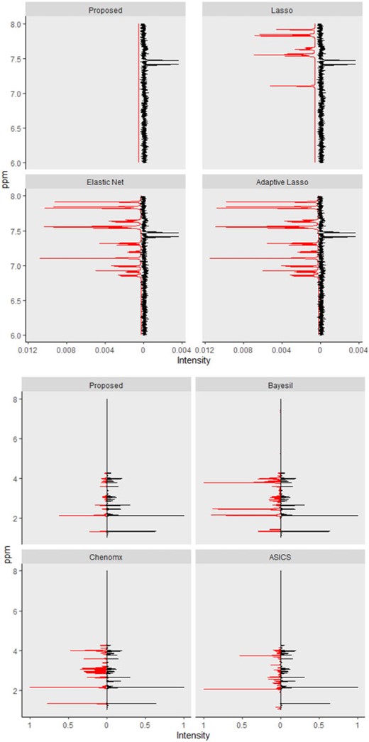
Top panel: Each fitted curve (left) generated from the proposed method, Lasso, elastic net, and adaptive Lasso is mirrored with the observed mixture spectrum (right). Bottom panel: Each fitted curve (left) generated from the proposed method, Bayesil, Chenomx, and ASICS is mirrored with the observed mixture spectrum (right).
The complexity level of a mixture spectrum also affected the accuracy and specificity. As the number of metabolites included in the mixture sample increased from 7 to 20 (Table 3), the accuracy decreased from 0.98 to 0.93 for the proposed method, from 0.93 to 0.81 for elastic net, and from 0.97 to 0.83 for Chenomx. Specificity encountered similar trends, with a drop from 0.97 to 0.85 for the proposed method, from 0.91 to 0.73 for the elastic net, and from 0.97 to 0.77 for Chenomx. Bayesil, Chenomx, and ASICS each used its own library of reference spectra which were collected at specific conditions (e.g., pH, temperature, etc.) to profile a given mixture spectrum. If the observed spectrum was collected under experimental conditions that were quite different from those in the reference libraries, it was possible that the induced shift variation was outside the range that these methods considered in their algorithms. This could consequentially cause failing to capture true metabolites (false negatives) and/or identifying wrong metabolites (false positives). Specifically, Table S13 of the Supplementary material available at Biostatistics online showed that Chenomx had a relatively lower number of false positives but it usually missed two to four metabolites across the three mixtures (e.g., L-alanine, L-cysteine, L-leucine, and L-glutamic acid).
On the other hand, Bayesil only failed to identify at most one metabolite (i.e., L-aspartic acid in the third mixture) while having a larger number of false positives (around 14-22). Finally, ASICS seemed to have both problems of missing true metabolites and identifying wrong metabolites. Figure 3 (right) mirrored the observed mixture spectrum with a fitted curve generated by the proposed method, Bayesil, Chenomx, and ASICS, respectively. More precisely, Figure S4 of the Supplementary material available at Biostatistics online zoomed in the spectral region from 1 to 4.5 ppm with the discrepancy between the observed and the profiled spectra to demonstrate the false positive and false negative effects on Bayesil, Chenomx, and ASICS as compared to the proposed approach.
5.2. Biological samples
Three serum samples of breast cancer patients from Hart and others (2017), which were publicly available on the MetaboLights database (Kale and others, 2016), were used to evaluate the practical application of the proposed method in comparison with the six other models. Evaluation criteria still included accuracy, sensitivity, and specificity, which were calculated using the metabolites manually identified by the authors of the study. According to Table 4, the proposed model yielded the best overall results with regard to identifying true metabolites in the mixtures while controlling the number of falsely identified metabolites. Similar to experimental results in Section 5.1, the six methods except for Chenomx identified more incorrect metabolites than the proposed approach. Specifically, the average sensitivity of our method was 0.70, while the remaining six approaches yielded an average sensitivity of less than 0.63. Across replications, Chenomx detected at most two metabolites out the total of 22 metabolites (|$<10\%$|) present in the mixture samples, which resulted in a low sensitivity of 0.05. Given the relatively low number of identified compounds, Chenomix, not surprisingly, produced the highest rate of specificity of 0.93.
Comparison of proposed method with Lasso, Elastic net, adaptive Lasso, Chenomx, Bayesil, and ASICS using three serum samples from breast cancer patients (Hart and others, 2017) and a library size of 104 metabolites. Performance was evaluated based on average accuracy, sensitivity, and specificity over the three empirical samples (N = 3). Corresponding standard deviations are recorded in parentheses
| Metrics | Proposed method | Lasso | Elastic Net | Adaptive Lasso | Chenomx | Bayesil | ASICS |
|---|---|---|---|---|---|---|---|
| Accuracy | 0.70 (0.01) | 0.65 (0.03) | 0.63 (0.04) | 0.66 (0.03) | 0.74 (0.02) | 0.46 (0.03) | 0.60 (0.01) |
| Sensitivity | 0.67 (0.03) | 0.67 (0.03) | 0.68 (0.00) | 0.67 (0.03) | 0.05 (0.04) | 0.55 (0.00) | 0.54 (0.03) |
| Specificity | 0.71 (0.01) | 0.65 (0.04) | 0.62 (0.05) | 0.66 (0.05) | 0.93 (0.04) | 0.43 (0.04) | 0.64 (0.02) |
Interestingly, there was a consistency across all methods with regard to failing to detect some of the metabolites that were previously identified by the authors of the original study. A signal-to-noise ratio (SNR) was calculated using TopSpin 4.06 (Bruker, Germany) for the mixture spectra. Three missed metabolites that included citric acid, formic acid, and phenylalanine, had a SNR less than 2. This is below the generally accepted lower-limits for peak detection.
ASICS had some built-in steps to exclude any reference metabolites from the library if at least one of its corresponding peaks did not show up in the observed complex spectrum. However, doing so could lead to eliminate some potential metabolites as it was quite possible for a given metabolite to lose one or more peaks due to experimental fluctuations (Zangger, 2015). This could potentially contributing to a large number of false negatives as seen in Table S13 of the Supplementary material available at Biostatistics online. Bayesil, on the other hand, did not integrate any regularization to reflect the sparsity of abundant metabolites in a complex mixture. As a result, Bayesil tended to identify more metabolites which were not part of the mixtures.
6. Conclusion
Metabolite identification and quantification play an essential role in any NMR metabolomics studies and are necessary to describe the underlying biological processes being investigated. However, manual assignment approaches are time-consuming, labor-intensive, and reliant on the knowledge and assessment of NMR experts. Many curve-fitting models with reference library support have been introduced to automate the metabolite identification process, but none has been unanimously demonstrated to be a gold standard approach in practice. We proposed a new approach that focused on addressing two major challenges of metabolite identification from complex mixtures: undesirable perturbations in signal locations and sparsity metabolites relative to reference databases. The proposed method was assessed using simulated, experimental and biological NMR metabolomics data sets. The overall performance was based on three metric including accuracy, sensitivity, and specificity. In addition, a comparison was made between the newly introduced approach and Lasso, elastic net, adaptive Lasso, Chenomx, Bayesil and ASICS with an increasing size of a reference library.
As a hybrid approach, the proposed leveraged sparsity properties from regularized models (e.g., Lasso, elastic net, and adaptive Lasso) which allowed a selection of potential metabolites from a large reference library. With the promising performance of our proposed method demonstrated using library size up to 200 (as shown in Table 3), this could potentially be scaled up to a relatively larger library. Additionally, our method incorporated a search window at each observed signal to capture any peak shifting which was then corrected for before estimating the metabolite concentration. Lastly, our approach with the modified objective function to correct for peak shifting and regularization enforcement was easy to implement. Though we empirically pre-selected some hyperparameters such as |$d$|, |$c_0$|, and |$\sigma_0$|, and |$\sigma_\epsilon$|, we demonstrated in the sensitivity analyses (Tables S4–S7 of the Supplementary material available at Biostatistics online) that these values did not affect our method performance much.
The proposed method showed the best results in capturing metabolites that were truly present in the mixtures while keeping incorrect assignments at a relatively lower level regardless of increasing shifting variations as demonstrated in the simulation studies. In addition, as the complexity of a mixture spectrum increased and the number of candidate metabolites grew larger, all methods shared a common trend of tending to identify more incorrect metabolites. In other words, the combination of the two factors resulted in lower accuracy and specificity for all models. It was interesting to see that the automated Profiler feature of Chenomx only assigned a small number of metabolites to the mixtures. Such conservative assignments ensured fewer false identifications, which in turn led to a higher specificity overall. However, Chenomx often failed at capturing some true metabolites leading to a low sensitivity. On the contrary, Bayesil’s aggressive detection yielded a large number of false positives while identifying most of the true positives. Consequently, Bayesil had a good sensitivity yet its specificity suffered considerably. Uniquely, ASICS seemed to encounter both problems of missing true metabolites and identifying wrong metabolites, resulting low sensitivity and specificity. Nonetheless, the new method still managed to maintain the best results across all three criteria (accuracy, sensitivity, and specificity) as compared to the others.
Even though we did not theoretically quantify the inferences of the regression coefficients in this article, we think it is possible to obtain proper confidence intervals for the coefficients, with special attention paid to the characteristics of the NMR spectral data. Again, as the final concentration estimation is conditional on both stages of the variable selection and covariate shifting correction, we utilize the random subsampling approach to closely investigate the stability of each stage. Based on the detailed results in Section 1.3 of the Supplementary material available at Biostatistics online, we observe that the two steps are stable in terms of selecting the true metabolites with a selection probability of at least 0.9, and estimating the covariate shifting error reasonably well. Such a stability procedure could be utilized to quantify the variability and construct confidence intervals for the metabolite concentration. Additionally, we could also leverage the jackknife resampling method, where each NMR peak is removed at a time to construct the jackknife confidence intervals. With regard to the nature of our proposed algorithm, the weights and the regression coefficients |${{\boldsymbol\beta}}$| are updated alternately at each coordinate descent step. More specifically, when the weights are updated using a new estimate of |${{\boldsymbol\beta}}$|, the objective function may not decrease. As a result, the objective function does not always decrease monotonically after each step; and we have noticed this phenomenon in Figure S1 of the Supplementary material available at Biostatistics online. Although our proposed algorithm is also not guaranteed to converge, we find that the numerical convergence is achieved in our simulation studies and real data analyses. Additionally, we choose the initial values |${{\boldsymbol\beta}}^{(0)} = 0_{p \times 1}$| in our numerical analyses due to a practical reason that a majority of metabolites are not present in a mixture (i.e., |$\beta_j = 0$|). Alternatively, we could also experiment with multiple initializations and select the ones which yield the smallest objective value. The theoretical convergence properties of the proposed method is important but is beyond the scope of this article and will be investigated in our future work.
Software
Corresponding code of the method in the form of GNU Octave is incorporated in a toolkit called MVAPACK (Worley and Powers, 2014), which is publicly available for academic users at http://bionmr.unl.edu/mvapack.php. The equivalent R code is available at https://github.com/thaovu1/SCRR.
Supplementary material
Supplementary material is available online at http://biostatistics.oxfordjournals.org.
Acknowledgments
The authors would like to thank the Associate Editor and two anonymous referees for their helpful and constructive comments, which led to a significant improvement of this article. We also thank Fatema Bhinderwala and Hannah Noel for generously providing us the experimental NMR mixture data sets.
Conflict of Interest: None declared.
Funding
The National Science Foundation (1660921); the Redox Biology Center (P30 GM103335, NIGMS), in part; and the Nebraska Center for Integrated Biomolecular Communication (P20 GM113126, NIGMS). The research was performed in facilities renovated with support from the National Institutes of Health (RR015468-01). Any opinions, findings, and conclusions or recommendations expressed in this material are those of the author(s) and do not necessarily reflect the views of the National Science Foundation.
