


Summary
Clinical trials often aim to compare two groups of patients for efficacy and/or toxicity depending on covariates such as dose. Examples include the comparison of populations from different geographic regions or age classes or, alternatively, of different treatment groups. Similarity of these groups can be claimed if the difference in average outcome is below a certain margin over the entire covariate range. In this article, we consider the problem of testing for similarity in the case that efficacy and toxicity are measured as binary outcome variables. We develop a new test for the assessment of similarity of two groups for a single binary endpoint. Our approach is based on estimating the maximal deviation between the curves describing the responses of the two groups, followed by a parametric bootstrap test. Further, using a two-dimensional Gumbel-type model we develop methodology to establish similarity for (correlated) binary efficacy–toxicity outcomes. We investigate the operating characteristics of the proposed methodology by means of a simulation study and present a case study as an illustration.
1. Introduction
A common problem in clinical drug development is the assessment of an investigational drug in two groups of patients, such as different age classes, gender, geographic regions, or different treatment groups (see Jhee and others, 2004; Otto and others, 2008) (among many others for clinical examples). A natural question is then whether the effect of the investigational drug is consistent across populations. Considering data with covariates, the effect of the investigational drug is described as a function of the covariates, and consistency across the two groups is claimed if these functions are similar in a suitable sense. Several authors use confidence bands for the difference between the response functions to construct such tests (see e.g., Liu and others, 2009; Gsteiger and others, 2011; Bretz and others, 2018). Alternatively, Dette and others (2018) and Möllenhoff and others (2018) propose more powerful tests by estimating a distance between the two functions, such as the squared integral of the difference or the maximal deviation between the functions. They claim similarity if the estimated distance is small.
All above approaches assume a single, continuous outcome. However, there are many situations where the efficacy of the drug to be investigated is defined by a binary outcome, such as tumor shrinkage or complete cure. In addition, many clinical trials involve the measurement of a second binary endpoint to assess the toxicity of the investigational drug, such as the occurrence of adverse events like fatigue or nausea. Hence the need arises to assess bivariate efficacy–toxicity outcomes which are likely to be correlated. Several methods for modeling multivariate binary outcomes have been proposed in the literature (see e.g., Glonek and McCullagh, 1995). Considering efficacy–toxicity outcomes, Murtaugh and Fisher (1990) and Heise and Myers (1996) investigate bivariate binary responses and derive optimal designs by fitting a bivariate logistic model and a Cox model to the data. Deldossi and others (2019) propose copulas to model the marginals and dependence structure of the outcomes separately. Further, Dragalin and Fedorov (2006) and Gaydos and others (2006) develop adaptive designs for identifying the optimal safe dose. Finally, several authors investigate the modeling and design of phase I/II dose finding trials incorporating bivariate outcomes using Bayesian methods (Zhang and others, 2006; Yin and others, 2006).
Different to the literature reviewed above, we investigate statistical tests to assess similarity of binary efficacy and toxicity responses for two groups of patients. Similarity can be claimed if the differences of both outcomes are below prespecified margins over the complete range of covariates. Accordingly, we first develop a new test of similarity for a single binary outcome. Second, we address similarity for bivariate binary (correlated) outcomes and develop a test for comparing simultaneously efficacy and toxicity outcomes among two populations. For this purpose, we use a two-dimensional Gumbel model (Gumbel, 1961) for bivariate logistic regression to model correlated bivariate binary endpoints. Our approach is based on a parametric bootstrap, which generates data under the constraint that the distances between the curves are precisely equal to the prespecified margins. We investigate finite sample properties and illustrate the procedures with a clinical trial example.
In a recent publication, Möllenhoff and others (2020) investigate the situation where some of the parameters of the models used to describe the dose-response relationship coincide (e.g., the placebo effect). They investigate continuous endpoints from two populations, propose a parametric bootstrap and demonstrate that using such additional information leads to more efficient statistical inference. In order to apply the methods proposed in this article to similar settings with additional toxicity outcomes, we will also extend our methodology to models with shared parameters and illustrate their use with the aforementioned clinical trial example.
2. Comparing curves for binary outcomes
In this section, we introduce a model-based approach for comparing the responses between two groups assuming binary outcomes. We consider models with covariates and assume for simplicity a one-dimensional covariate, although the proposed methodology applies more broadly. For both groups, we choose the covariate space as a dose range |$\cal{D}$| and assume that the groups are investigated at |$k_\ell$| dose levels |$d_{\ell,1},\ldots,d_{\ell,k_\ell}$|, |$\ell=1,2$|, where the index |$\ell=1,2$| is the group indicator. More precisely the dose range is given by all dose levels between the lowest and highest dose across both two groups, that is |$\mathcal D=\left[ \min_{\ell= 1,2 } d_{\ell,1}, \max_{\ell=1,2} d_{\ell,k_\ell} \right]$|. Often |$\min_{\ell= 1,2 } d_{\ell,1}=0$| is the placebo or zero-dose control group. The highest dose level |$\max_{\ell=1,2} d_{\ell,k_\ell}$| is often determined in earlier trials investigating the tolerability or safety of a compound. Note that clinical trials typically randomize patients to a few fixed dose levels, which have to be determined in advance, such that |$k_\ell$| is often in the range of 4–6 (Bretz and others, 2005).
The following algorithm provides a bootstrap test for the hypotheses (2.3). It is derived by adapting the methodology developed in Dette and others (2018) to binary data.
- (1) Calculate the MLE |$(\hat\beta_{\ell},\hat\gamma_{\ell})$|, |$\ell=1,2$|, by maximizing for each group the log-likelihood given in (2.2). The test statistic is obtained by$$\hat \Delta^E:=\max_{d\in \cal D}\left| \eta^E_1(d,\hat\beta_{1},\hat\gamma_{1})-\eta^E_2(d,\hat\beta_{2},\hat\gamma_{2})\right|.$$
- (2) Define estimators of the parameters |$\beta_\ell, \gamma_\ell,\ \ell=1,2$|, so that the corresponding curves fulfill the null hypothesis (2.3), that iswhere |$(\bar\beta_1,\bar\gamma_{1})$| and |$(\bar\beta_{2},\bar\gamma_{2})$| maximize the same objective function as defined in (2.2), but under the constraint$$\begin{equation} \label{MLcons} \big(\hat{\hat{\beta}}_{\ell},\hat{\hat{\gamma}}_{\ell}\big)= \left\{ \begin{array} {ccc} (\hat\beta_{\ell},\hat\gamma_{\ell}) & \mbox{if} & \hat \Delta^E \geq \varepsilon^E \nonumber \\ (\bar\beta_{\ell},\bar\gamma_{\ell})& \mbox{if} & \hat \Delta^E < \varepsilon^E \end{array} \right. \quad \ell=1,2, \end{equation}$$(2.4)$$\begin{equation}\label{constr} \Delta^E=\max_{d\in \mathcal{D}} \left| \eta^E_1(d,\beta_{1},\gamma_{1})-\eta^E_2(d,\beta_{2},\gamma_{2})\right|= \epsilon^E. \end{equation}$$We discretize the dose range |${\cal D}$| to get a feasible optimization problem by fixing |$r$| nodes |$d_1,\dots,d_r$| and using a smooth approximation of the maximum,in (2.4). We solve the constrained optimization problem by using the augmented Lagrangian minimization algorithm as implemented with the auglag() function in the R package alabama (Varadhan, 2014).$$\max{(d_1,\ldots,d_r)} \approx \lambda\log{\sum_{i=1}^r\exp{\tfrac{d_i}{\lambda}}}\text{ for }$\lambda \to 0$,$$
(3) Proceed as follows:
(i) Generate bootstrap data under the null hypothesis (2.3) by creating binary data specified by the parameters |$\big(\hat{\hat{\beta}}_{\ell},\hat{\hat{\gamma}}_{\ell}\big)$|, |$\ell=1,2$|. More precisely, calculate |$\eta^E_\ell(d_{\ell,i},\hat{\hat{\beta}}_{\ell},\hat{\hat{\gamma}}_{\ell})$|, |$i=1,\ldots,k_\ell,\ \ell=1,2$| yielding the probabilities |$p(d_{\ell,i})$| at each dose level |$d_{\ell,i} $|.
- (ii) From the bootstrap data calculate the MLE |$(\hat\beta_{\ell}^*,\hat\gamma_{\ell}^*)$| as in step |$(1)$| and the test statistic(2.5)$$\begin{eqnarray}\label{boot}\hat \Delta^{E*}=\max_{d\in \cal D}\left| \eta^E_1(d,\hat\beta^*_{1},\hat\gamma^*_{1})-\eta^E_2(d,\hat\beta^*_{2},\hat\gamma^*_{2})\right|. \end{eqnarray}$$
- (iii) Repeat the steps (i) and (ii) |$n_{boot}$| times to generate replicates |$\hat \Delta^{E*}_{1}, \dots, \hat \Delta^{E*}_{n_{boot}}$| of |$\hat \Delta^{E*}$|. Let |$\hat \Delta^{E*}_{(1)} \le \ldots \le \hat \Delta^{E*}_{(n_{boot})}$| denote the corresponding order statistic. The estimator of the |$\alpha$|-quantile of the distribution of |$\hat \Delta^{*}$| is defined by |$\hat \Delta^{E*}_{(\lfloor n_{boot} \alpha \rfloor )}$|. Reject the null hypothesis (2.3) and decide for similarity if(2.6)$$\begin{equation} \label{testInf} \hat \Delta^E < \hat \Delta^{E*}_{(\lfloor n_{boot} \alpha \rfloor )}. \end{equation}$$
Alternatively, calculate the |$p$|-value |$\hat F_{n_{boot}}^E(\hat \Delta^E) = {\frac{1}{n_{boot}}} \sum_{i=1}^{n_{boot}} I\{ \hat \Delta^{E*}_{i} \leq \hat \Delta^E\}$| and reject the null hypothesis (2.3) if |$\hat F_{n_{boot}}^E(\hat \Delta^E)<\alpha$| for a prespecified significance level |$\alpha$|, where |$\hat F_{n_{boot}}^E$| denotes the empirical distribution function of the bootstrap sample.
Both, the bootstrap quantile |$\hat \Delta^{E*}_{(\lfloor n_{boot} \alpha \rfloor )}$| and the |$p$|-value |$\hat F_{n_{boot}}^E(\hat \Delta^E)$|, depend on the number of bootstrap replicates |$n_{boot}$| and the margin |$\varepsilon^E$| given in the hypotheses (2.3), but we do not reflect the latter dependence in our notation.
3. Tests for similarity of efficacy–toxicity responses
3.1. The Gumbel model for efficacy–toxicity outcomes
Note that the marginal distributions are logistic and that the parameter |$\nu$| represents the dependence of |$U$| and |$V$|, where |$\nu=0$| corresponds to independent margins and in this case, two separate logistic models for efficacy and toxicity can be fitted separately to the data. The approach in this article can also be applied to other parametric two-dimensional distributions. In the Supplementary material available at Biostatistics online, we investigate an alternative distribution with logistic margins and a different dependence structure.
3.2. The test procedure
As the global null in (3.7) is the union of |$H_0^E$| and |$H_0^T$| we can apply the intersection union principle (Berger, 1982). That is, we reject the global null in (3.7) and claim similarity only if both individual null hypotheses in (3.9) and (3.10) are rejected. Each of the two individual tests in (3.9) and (3.10) is performed by extending the parametric bootstrap approach in Algorithm 2.1, as described below.
- (1) Calculate the MLE |$\hat \theta_\ell=(\hat\beta_{\ell,1},\hat\gamma_{\ell,1},\hat\beta_{\ell,2},\hat\gamma_{\ell,2},\hat\nu_{\ell})$|, |$\ell=1,2$|, by maximizing the log-likelihood given in (3.6) for each group. The test statistics are obtained byand$$\hat \Delta^E=\Delta^E(\hat\theta_1,\hat\theta_2)=\max_{d\in \cal D}\big| \eta_1^E(d,\hat\theta_1)-\eta_2^E(d,\hat\theta_2)\big|$$$$\hat \Delta^T=\Delta^T(\hat\theta_1,\hat\theta_2)=\max_{d\in \cal D}\big| \eta_1^T(d,\hat\theta_1)-\eta_2^T(d,\hat\theta_2)\big|.$$
(2) For each individual test in (3.9) and (3.10) we perform a constrained optimization as described in Algorithm 2.1, yielding estimates |$\hat{\hat{\theta}}_{\ell}$|, |$\ell=1,2$|. This procedure is done separately for each individual test because the constraints differ. Although the constraints are only imposed on the marginal densities which do not contain the dependence parameters |$\nu_{\ell}$|, they appear in the likelihood function to be maximized under the constraints. Consequently the constrained estimates of the parameters |$\nu_{\ell}$| are usually different from the unconstrained estimates. We generate bootstrap data for each individual test separately and obtain replicates |$\hat \Delta^{E*}_{1}, \dots, \hat \Delta^{E*}_{n_{boot}}$| for the comparison of the efficacy curves and |$\hat \Delta^{T*}_{1}, \dots, \hat \Delta^{T*}_{n_{boot}}$| for the comparison of the toxicity curves. Let |$\hat \Delta^{E*}_{(1)} \le \ldots \le \hat \Delta^{E*}_{(n_{boot})}$| and |$\hat \Delta^{T*}_{(1)} \le \ldots \le \hat \Delta^{T*}_{(n_{boot})}$| denote the corresponding order statistics and let |$\hat \Delta^{E*}_{(\lfloor n_{boot} \alpha \rfloor )}$| and |$\hat \Delta^{T*}_{(\lfloor n_{boot}\alpha \rfloor )}$| denote the corresponding empirical level |$\alpha$| quantiles, respectively.
- (3) Reject the global null hypothesis (3.7) if(3.11)$$\begin{equation} \label{testInf2} \hat \Delta^E < \hat \Delta^{E*}_{(\lfloor n_{boot} \alpha \rfloor )}~~ \text{ and } ~~ \hat \Delta^T < \hat \Delta^{T*}_{(\lfloor n_{boot}\alpha \rfloor )}. \end{equation}$$
We do not need to adjust the level of the two individual tests and can thus use the |$\alpha$|-quantile according to the intersection union principle. The technical difficulty of the implementation of this algorithm consists in generating bivariate correlated binary data in Step (2), which is explained in more detail in the following section.
3.3. Generation of bivariate correlated binary data
Here, |$p_1(d)=\eta^E(d,\theta_1)$| and |$p_2(d)=\eta^T(d,\theta_2)$| denote the marginal probabilities of efficacy and toxicity, respectively. These restrictions have to be fulfilled at each dose in order to guarantee that a joint distribution of |$Y^E$| and |$Y^T$| can exist. We impose these inequality constraints in the optimization step in addition to the constraint described in (2.4) such that the estimates |$\hat{\hat{\theta}}_1$| and |$\hat{\hat{\theta}}_2$| generate a distribution and bootstrap data can be obtained.
3.4. Shared parameters
As pointed out in the introduction there exist also situations, where it is reasonable to assume that certain model parameters are the same for both groups. In such cases, the total number of parameters to be estimated is reduced, which yields to more efficient inference if the assumption is correct. For example, Möllenhoff and others (2020) describe a trial assessing similarity of Japanese and Caucasian patients, where a similar response to placebo and a common maximum treatment effect is assumed.
The new methodology can be further developed to address this situation by considering a joint likelihood function instead of fitting two separate models. For this purpose, we adopt Algorithm 3.1 to that situation as follows. Let |$\theta=(\theta_0,\tilde\theta_1,\tilde\theta_2)$|, where |$\theta_0$| denotes the vector of common parameters and |$\tilde\theta_1, \tilde\theta_2$| denote the remaining parameters of the Gumbel models, such that |$\theta_\ell=(\theta_0,\tilde\theta_\ell)$|, |$\ell=1,2$|. We then estimate an MLE |$\hat\theta$| by using the combined sample and maximizing |$l_1(\theta_0,\tilde\theta_1)+l_2(\theta_0,\tilde\theta_2)$|, where |$l_1$| and |$l_2$| are the log-likelihood functions given in (3.6). The calculation of the test statistic, the constrained optimization, and the generation of bootstrap data described in step (2) of Algorithm 3.1 are performed similarly, now using joint likelihood functions instead of fitting two separate models throughout. The details are omitted for the sake of brevity.
4. Finite sample properties
We now investigate the finite sample properties of the two tests based on Algorithms 2.1 and 3.1. We consider the dose range |$\mathcal{D}=[ 0, 2 ] $| with the seven dose levels |$0, 0.1, 0.2, 0.5, 1, 1.5,$| and |$2$|. We assume |$n_{\ell,i}=7,\ 14,\ 21,\ 28,\ 50$| patients per dose level, |$i=1,\ldots, 7$| and group |$\ell=1,2$|, resulting in |$n_\ell=49,98,147,196, 350$|, |$\ell=1,2$|. The significance level is |$\alpha=0.05$| throughout and we consider three different margins in (3.7) and (3.8), that is |$0.1$|, |$0.15,$| and |$0.2$|. All simulations are performed using |$1000$| simulation runs and |$n_{boot}=400$| bootstrap replications. Binary data are generated as described in Section 3.3. We set |$\nu=0$| for the univariate (efficacy) case. For the sake of brevity, we present in this section only the results for the bivariate case and a short summary of the findings for the univariate case. We refer to Supplementary Section S1 available at Biostatistics online for the complete simulation results and a more detailed discussion.
4.1. Univariate efficacy outcomes
Supplementary Table S1 and Table S2 available at Biostatistics online display the simulated Type I error rates and the power of the bootstrap test (2.6), respectively, for margins |$\epsilon^E=0.1$|, |$0.15$|, |$0.2$|. We conclude that the test controls its level in all cases under consideration. The approximation of the level is very precise at the margin of the null hypothesis (that is, |$\Delta^E=\epsilon^E$|) and this accuracy increases with increasing sample sizes. Moreover, in the interior of the null hypothesis (that is, |$\Delta^E > \epsilon^E$|) the number of rejections is close to 0 in all scenarios, indicating that the Type I error rate is very small in these cases. We further conclude that the procedure has reasonable power for sufficiently large sample sizes. For example, the test achieves more than |$80\%$| power for sample sizes of |$28$| or |$50$| patients per dose level, depending on the margin under consideration. We also observe that the power increases with increasing sample sizes.
4.2. Bivariate efficacy–toxicity outcomes
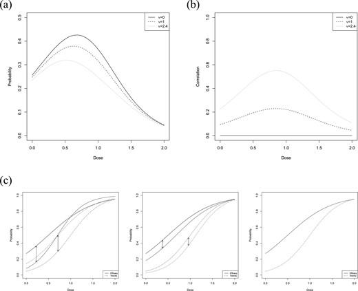
(a) Probability |$\mathbb{P}(Y^E=1, Y^T=0 )=p_{10}(d)$| in dependence of the dose for the reference model (4.1) for different choices of the correlation parameter |$\nu$|; (b) Correlation of efficacy and toxicity response for different choices of |$\nu$| in dependence of the dose; (c) Efficacy curves (solid lines) and toxicity curves (dashed lines) derived in (3.3). The black lines correspond to the reference model, the blue lines to the second model, specified by |$\theta_2$|. The scenarios shown correspond to a maximum absolute deviation (indicated by the arrows) of |$\Delta^E=\Delta^T=0.2,\ 0.1$| and |$0$| (from left to right).
| |$\theta_1$| | |$\theta_2$| | |$\Delta=(\Delta^E,\Delta^T)$| | |
|---|---|---|---|
| Alternative | |$(-1,2,-3,3,\nu_1)$| | |$(-1,2,-3,3,\nu_2)$| | |$(0,0)$| |
| |$(-1,2,-3,3,\nu_1)$| | |$(-1.2,2,-3.3,3.1,\nu_2)$| | |$(0.05,0.05)$| | |
| |$(-1,2,-3,3,\nu_1)$| | |$(-1.5,2.2,-3.6,3.2,\nu_2)$| | |$(0.1,0.1)$| | |
| Null hypothesis | |$(-1,2,-3,3,\nu_1)$| | |$(-2,3.4,-2,2.5,\nu_2)$| | |$(0.15,0.15)$| |
| |$(-1,2,-3,3,\nu_1)$| | |$(-1,2,-2,2.5,\nu_2)$| | |$(0,0.15)$| | |
| |$(-1,2,-3,3,\nu_1)$| | |$(-2.4,3.4,-1.8,2.5,\nu_2)$| | |$(0.2,0.2)$| | |
| |$(-1,2,-3,3,\nu_1)$| | |$(-1,2,-1.8,2.5,\nu_2)$| | |$(0,0.2)$| |
For the Type I error rate simulations, we counted the number of individual and simultaneous rejections of both null hypotheses in (3.9) and (3.10), allowing us to reject the global null hypothesis in (3.7). All simulation results are displayed in Tables 2 and 3, where the numbers in brackets correspond to the proportion of rejections for the individual tests on efficacy and toxicity. For the sake of brevity, we assume only two different margins |$\epsilon=(\epsilon^E,\epsilon^T)=(0.15,0.15)$| and |$(0.2,0.2)$|. We observe that the global bootstrap test according to Algorithm 3.1 is rather conservative as the Type I error rates are very small. For example, for |$n_{\ell,i}=14$|, |$\nu_1=\nu_2=1$| and |$\Delta=(\Delta^E,\Delta^T)=\epsilon=(0.2,0.2)$| the individual proportions of rejection are |$0.046$| for efficacy and |$0.058$| for toxicity, whereas the Type I error rate for the global test is |$0.001$|, which is well below the nominal level. This is a common feature of the intersection union principle for the problem of testing equivalence in multivariate responses (Berger and Hsu, 1996). A similar conclusion holds for the high level of dependence, that is |$\nu_1=\nu_2=2.4$|. Considering the same configuration as above, that is |$n_{\ell,i}=14$| and |$\Delta=\epsilon=(0.2,0.2)$|, the individual proportions of rejection are |$0.088$| for efficacy and |$0.089$| for toxicity, whereas the Type I error rate for the global test is |$0.002$|.
Simulated Type I error rates of the global bootstrap test (3.11) for two different choices of |$\nu_\ell,\ \ell=1,2$|
| |$\epsilon=(\epsilon^E,\epsilon^T)$| | |$n_{\ell,i}$| | |$\theta_2$| | |$\Delta=(\Delta^E,\Delta^T)$| | |$\nu_\ell=1$| | |$\nu_\ell=2.4$| |
|---|---|---|---|---|---|
| |$(0.15,0.15)$| | |$7$| | |$(-2,3.4,-2,2.5,\nu_2)$| | |$(0.15,0.15)$| | 0.001 (0.063/0.074) | 0.006 (0.078/0.064) |
| |$(-1,2,-2,2.5,\nu_2)$| | |$(0,0.15)$| | 0.008 (0.122/0.060) | 0.012 (0.112/0.075) | ||
| |$14$| | |$(-2,3.4,-2,2.5,\nu_2)$| | |$(0.15,0.15)$| | 0.003 (0.040/0.047) | 0.003 (0.082/0.065) | |
| |$(-1,2,-2,2.5,\nu_2)$| | |$(0,0.15)$| | 0.001 (0.207/0.052) | 0.020 (0.230/0.068) | ||
| |$21$| | |$(-2,3.4,-2,2.5,\nu_2)$| | |$(0.15,0.15)$| | 0.000 (0.026/0.046) | 0.002 (0.051/0.057) | |
| |$(-1,2,-2,2.5,\nu_2)$| | |$(0,0.15)$| | 0.016 (0.325/0.041) | 0.029 (0.326/0.084) | ||
| |$28$| | |$(-2,3.4,-2,2.5,\nu_2)$| | |$(0.15,0.15)$| | 0.000 (0.049/0.053) | 0.004 (0.125/0.090) | |
| |$(-1,2,-2,2.5,\nu_2)$| | |$(0,0.15)$| | 0.032 (0.476/0.058) | 0.034 (0.455/0.076) | ||
| |$50$| | |$(-2,3.4,-2,2.5,\nu_2)$| | |$(0.15,0.15)$| | 0.000 (0.035/0.078) | 0.012 (0.210/0.084) | |
| |$(-1,2,-2,2.5,\nu_2)$| | |$(0,0.15)$| | 0.074 (0.827/0.085) | 0.089 (0.815/0.111) | ||
| |$(0.2,0.2)$| | |$7$| | |$(-2.4,3.4,-1.8,2.5,\nu_2)$| | |$(0.2,0.2)$| | 0.004 (0.061/0.063) | 0.006 (0.091/0.101) |
| |$(-1,2,-1.8,2.5,\nu_2)$| | |$(0,0.2)$| | 0.012 (0.218/0.055) | 0.019 (0.233/0.084) | ||
| |$14$| | |$(-2.4,3.4,-1.8,2.5,\nu_2)$| | |$(0.2,0.2)$| | 0.001 (0.046/0.058) | 0.002 (0.088/0.089) | |
| |$(-1,2,-1.8,2.5,\nu_2)$| | |$(0,0.2)$| | 0.024 (0.396/0.067) | 0.027 (0.442/0.065) | ||
| |$21$| | |$(-2.4,3.4,-1.8,2.5,\nu_2)$| | |$(0.2,0.2)$| | 0.003 (0.048/0.070) | 0.003 (0.090/0.087) | |
| |$(-1,2,-1.8,2.5,\nu_2)$| | |$(0,0.2)$| | 0.033 (0.672/0.051) | 0.040 (0.648/0.070) | ||
| |$28$| | |$(-2.4,3.4,-1.8,2.5,\nu_2)$| | |$(0.2,0.2)$| | 0.003 (0.069/0.072) | 0.004 (0.124/0.077) | |
| |$(-1,2,-1.8,2.5,\nu_2)$| | |$(0,0.2)$| | 0.050 (0.813/0.065) | 0.068 (0.870/0.078) | ||
| |$50$| | |$(-2.4,3.4,-1.8,2.5,\nu_2)$| | |$(0.2,0.2)$| | 0.004 (0.054/0.076) | 0.003 (0.145/0.103) | |
| |$(-1,2,-1.8,2.5,\nu_2)$| | |$(0,0.2)$| | 0.060 (0.982/0.061) | 0.127 (0.986/0.132) |
Simulated power of the global bootstrap test (3.11) for two different choices of |$\nu_\ell,\ \ell=1,2$|
| |$\epsilon=(\epsilon^E,\epsilon^T)$| | |$n_{\ell,i}$| | |$\theta_2$| | |$\Delta=(\Delta^E,\Delta^T)$| | |$\nu_\ell=1$| | |$\nu_\ell=2.4$| |
|---|---|---|---|---|---|
| |$(0.15,0.15)$| | |$7$| | |$(-1.5,2.2,-3.6,3.2,\nu_2)$| | |$(0.1,0.1)$| | 0.009 (0.092/0.125) | 0.007 (0.089/0.125) |
| |$(-1.2,2,-3.3,3.1,\nu_2)$| | (0.05,0.05) | 0.009 (0.129/0.108) | 0.010 (0.114/0.116) | ||
| |$(-1,2,-3,3,\nu_2)$| | |$(0,0)$| | 0.002 (0.128/0.133) | 0.018 (0.153/0.121) | ||
| |$14$| | |$(-1.5,2.2,-3.6,3.2,\nu_2)$| | |$(0.1,0.1)$| | 0.008 (0.105/0.102) | 0.014 (0.119/0.104) | |
| |$(-1.2,2,-3.3,3.1,\nu_2)$| | |$(0.05,0.05)$| | 0.031 (0.176/0.146) | 0.042 (0.183/0.172) | ||
| |$(-1,2,-3,3,\nu_2)$| | |$(0,0)$| | 0.035 (0.196/0.162) | 0.045 (0.209/0.214) | ||
| |$21$| | |$(-1.5,2.2,-3.6,3.2,\nu_2)$| | |$(0.1,0.1)$| | 0.020 (0.145/0.150) | 0.025 (0.145/0.155) | |
| |$(-1.2,2,-3.3,3.1,\nu_2)$| | |$(0.05,0.05)$| | 0.051 (0.288/0.201) | 0.075 (0.242/0.254) | ||
| |$(-1,2,-3,3,\nu_2)$| | |$(0,0)$| | 0.085 (0.345/0.265) | 0.077 (0.309/0.269) | ||
| |$28$| | |$(-1.5,2.2,-3.6,3.2,\nu_2)$| | |$(0.1,0.1)$| | 0.038 (0.185/0.166) | 0.057 (0.137/0.189) | |
| |$(-1.2,2,-3.3,3.1,\nu_2)$| | |$(0.05,0.05)$| | 0.098 (0.387/0.266) | 0.121 (0.356/0.313) | ||
| |$(-1,2,-3,3,\nu_2)$| | |$(0,0)$| | 0.201 (0.484/0.385) | 0.202 (0.453/0.403) | ||
| |$50$| | |$(-1.5,2.2,-3.6,3.2,\nu_2)$| | |$(0.1,0.1)$| | 0.066 (0.295/0.263) | 0.106 (0.239/0.234) | |
| |$(-1.2,2,-3.3,3.1,\nu_2)$| | |$(0.05,0.05)$| | 0.318 (0.624/0.484) | 0.326 (0.565/0.527) | ||
| |$(-1,2,-3,3,\nu_2)$| | |$(0,0)$| | 0.566 (0.842/0.656) | 0.581 (0.827/0.686) | ||
| |$(0.2,0.2)$| | |$7$| | |$(-1.5,2.2,-3.6,3.2,\nu_2)$| | |$(0.1,0.1)$| | 0.018 (0.133/0.140) | 0.029 (0.159/0.129) |
| |$(-1.2,2,-3.3,3.1,\nu_2)$| | (0.05,0.05) | 0.027 (0.159/0.151) | 0.032 (0.213/0.155) | ||
| |$(-1,2,-3,3,\nu_2)$| | |$(0,0)$| | 0.026 (0.183/0.189) | 0.049 (0.221/0.191) | ||
| |$14$| | |$(-1.5,2.2,-3.6,3.2,\nu_2)$| | |$(0.1,0.1)$| | 0.063 (0.277/0.210) | 0.076 (0.278/0.230) | |
| |$(-1.2,2,-3.3,3.1,\nu_2)$| | |$(0.05,0.05)$| | 0.112 (0.352/0.299) | 0.099 (0.335/0.282) | ||
| |$(-1,2,-3,3,\nu_2)$| | |$(0,0)$| | 0.124 (0.409/0.300) | 0.171 (0.451/0.356) | ||
| |$21$| | |$(-1.5,2.2,-3.6,3.2,\nu_2)$| | |$(0.1,0.1)$| | 0.119 (0.369/0.310) | 0.142 (0.343/0.321) | |
| |$(-1.2,2,-3.3,3.1,\nu_2)$| | |$(0.05,0.05)$| | 0.243 (0.585/0.388) | 0.254 (0.527/0.416) | ||
| |$(-1,2,-3,3,\nu_2)$| | |$(0,0)$| | 0.328 (0.658/0.505) | 0.322 (0.593/0.536) | ||
| |$28$| | |$(-1.5,2.2,-3.6,3.2,\nu_2)$| | |$(0.1,0.1)$| | 0.177 (0.468/0.348) | 0.212 (0.429/0.418) | |
| |$(-1.2,2,-3.3,3.1,\nu_2)$| | |$(0.05,0.05)$| | 0.445 (0.716/0.608) | 0.472 (0.688/0.622) | ||
| |$(-1,2,-3,3,\nu_2)$| | |$(0,0)$| | 0.541 (0.816/0.660) | 0.581 (0.822/0.705) | ||
| |$50$| | |$(-1.5,2.2,-3.6,3.2,\nu_2)$| | |$(0.1,0.1)$| | 0.404 (0.717/0.543) | 0.437 (0.653/0.602) | |
| |$(-1.2,2,-3.3,3.1,\nu_2)$| | |$(0.05,0.05)$| | 0.740 (0.933/0.783) | 0.765 (0.897/0.836) | ||
| |$(-1,2,-3,3,\nu_2)$| | |$(0,0)$| | 0.900 (0.987/0.914) | 0.933 (0.985/0.945) |
In general, we conclude that for a low level of dependence the individual tests on efficacy and toxicity yield rejection probabilities that are close to |$0.05$| when simulating on the margin of the global null hypothesis (that is |$\Delta=\epsilon$|) and hence the global Type I error rates are well below |$\alpha$| in these cases. However, for a high level of correlation, that is |$\nu_1=\nu_2=2.4$|, there are a few scenarios where the Type I error rate is too large. For instance, we observe the largest proportion of rejections of the global null hypothesis given by |$0.127$| for |$n_{\ell,i}=50$|, |$\epsilon=(0.2,0.2)$| and |$\Delta=(0,0.2)$|. Considering the same configurations but |$\epsilon=(0.15,0.15)$|, yields a proportion of |$0.089$|, which is lower but still above the desired value of |$0.05$|. For all other scenarios, the Type I error of the global test is well below the nominal level. The size of the parameter |$\nu_\ell$| affects the precision of the estimates for the parameter |$\theta_\ell$| of the Gumbel model, which explains the different results for the rather low correlations corresponding to |$\nu_\ell=1$| and the high correlations obtained for |$\nu_\ell=2.4$|, |$\ell=1,2$|. In other words, a high correlation makes the estimation of the curves more difficult, even for large sample sizes. A more detailed discussion, including a table presenting the bias of the estimates for some configurations, can be found in Supplementary Section S3 available at Biostatistics online.
The simulated power is shown in Table 3. It turns out that the global test achieves reasonable power for sufficiently large sample sizes. For example, a maximum power (always attained at |$\Delta=(0,0)$|) of |$0.933$| is achieved for the global test for a choice of |$n_{\ell,i}=50$|, |$\nu_1=\nu_2=2.4,$| and |$\epsilon=(0.2,0.2)$|. For a lower margin, that is, |$\epsilon=(0.15,0.15)$|, the maximum power is smaller, but still increasing with growing sample sizes, reaching for instance |$0.581$| for |$n_{\ell,i}=50$| and |$\nu_1=\nu_2=2.4$|. The same statement holds for a lower correlation of |$\nu_\ell=1,\ \ell=1,2$|. For example, considering |$n_{\ell,i}=28$|, |$\nu_1=\nu_2=1$| and |$\epsilon=(0.2,0.2)$|, we observe a maximum power of |$0.541$|.
5. Case study
To illustrate the proposed methodology, we consider an example that is inspired by a recent consulting project of one of the authors. A nonsteroidal anti-inflammatory drug is to be investigated for its ability to attenuate dental pain after the removal of two or more impacted third molar teeth. Dental pain is a common and inexpensive setting for analgesic proof of concept, recruitment being fast and the outcome being measured within a few hours. It is common to measure the pain intensity on an ordinal scale at baseline and several times after the administration of a single dose. The pain intensity difference from baseline, averaged over several hours after drug administration, may then be compared with a clinical relevance threshold to create a binary success variable for efficacy. In this particular setting, side effects such as nausea and sedation after dosing were anticipated, resulting in a binary toxicity variable whether the patient experienced any such adverse events. As approved analgesics with an identified dosing range and a known dose-response relationship for tolerability are available, the objective of the study at hand was to demonstrate similarity with a marketed product for the bivariate efficacy–toxicity outcome in a proof of concept setting.
This was a randomized double-blind multi-regional parallel group clinical trial with a total of 300 patients being allocated to either placebo or one of four active doses coded as |$0.05$|, |$0.20$|, |$0.50$|, and |$1$| (for the investigational drug) and |$0.10$|, |$0.30$|, |$0.60$|, and |$1$| (for the marketed product), resulting in |$n = 30$| per group (assuming equal allocation). To maintain confidentiality, the actual doses have been scaled to lie within the |$[0, 1]$| interval. Since the study has not been completed yet, we use a hypothetical data set to illustrate the proposed methodology.
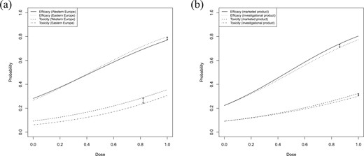
(a) Efficacy and toxicity curves corresponding to the fitted Gumbel models (5.1) for the hypothetical data described in Section 5. The solid (efficacy) and the dashed line (toxicity) correspond to the patients from Western Europe, the dotted (efficacy) and the dotted-dashed (toxicity) to those from Eastern Europe. (b) Efficacy and toxicity curves under the assumption of shared placebo parameters. Here the solid (efficacy) and the dashed line (toxicity) correspond to the marketed product, the dotted (efficacy) and the dotted-dashed (toxicity) to the investigational drug, respectively. The arrows indicate the maximum absolute distances.
Using |$n_{boot}=1000$| bootstrap replications, we obtain critical values |$q_{0.05}^E=0.061$| and |$q_{0.05}^T=0.056$| and test the global null hypothesis (3.7) against the alternative (3.8). Since |$\hat \Delta^E=0.029< 0.061=\hat q_{0.05}^E$| and |$\hat \Delta^T=0.051< 0.056=\hat q_{0.05}^T$|, we can reject (3.7) at level |$\alpha = 0.05$|. This conclusion can also be drawn by directly considering the |$p$|-values obtained from the empirical distribution functions of the bootstrap sample according to Step (iii) of Algorithm 2.1. In general, we reject the null hypothesis (3.7) at level |$\alpha$| if the maximum of the two individual |$p$|-values for (3.9) and (3.10) is smaller than or equal to |$\alpha$|. Since the individual |$p$|-values are given by |$\hat F_{n_{boot}}^E(\hat \Delta^E)=0.015$| and |$\hat F_{n_{boot}}^T(\hat \Delta^T)=0.042$|, we have |$\max{(0.015,0.042)}=0.042 < 0.05 = \alpha$| and can reject the null hypothesis (3.7), thus concluding similarity of efficacy and toxicity across the two geographic regions.
Based on this result, it is therefore reasonable to proceed with a further analysis of this trial using the data pooled from both regions. We now compare the investigational drug with the marketed product across all dose levels for the bivariate efficacy–toxicity outcomes of all |$300$| patients randomized into the study. For this analysis, it is reasonable to assume that the placebo effect is the same for both products with regard to efficacy and toxicity and to investigate the question of similarity under the assumption of shared placebo parameters as described in Section 3.4. More precisely we assume that |$\beta_{1,1}=\beta_{2,1}$| and |$\beta_{1,2}=\beta_{2,2}$|, which reduces the number of parameters to be estimated from |$10$| to |$8$|. The parameter estimates are |$\hat\theta_1=(-1.250, 2.661, -2.299, 1.564, -0.066)$| and |$\hat\theta_2=(-1.250, 2.481, -2.299, 1.453, 0.941)$|, see Figure 2(b) for the corresponding efficacy and toxicity curves. The maximum distances are now given by |$\hat \Delta^E=0.031$| and |$\hat \Delta^T=0.024$|, attained at the dose levels |$0.86$| and |$1$|, respectively. We perform the test at a significance level of |$\alpha=0.05$| and generate bootstrap data under the assumption of common placebo parameters. The critical values are now given by |$q_{0.05}^E=0.060$| and |$q_{0.05}^T=0.035$| and hence we conclude that the null hypothesis (3.7) can be rejected as |$\hat \Delta^E=0.031< \hat q_{0.05}^E=0.06$| and |$\hat \Delta^T=0.024< \hat q_{0.05}^T=0.035$|. The |$p$|-values are given by |$\hat F_{n_{boot}}^E(\hat \Delta^E)=0.021$| and |$\hat F_{n_{boot}}^T(\hat \Delta^T)=0.031$|, respectively.
Finally, we note that fitting separate models as shown above also implies that the dependence parameter is allowed to differ between the two drugs. Such an approach seems sensible in practice as it would be hard to justify clinically that the dependence parameter is the same, unless the two products are from the same chemical class or have a common mode of action. If for a given problem at hand it can be argued in favor of a shared dependence parameter then the methods in this article can be extended following Möllenhoff and others (2020).
6. Conclusions and discussion
In the first part of this article, we investigated a single efficacy response given by a binary outcome and derived a test procedure for the similarity of the corresponding dose-response curves, which can be modeled, for instance, by a parametric logistic regression or a probit model. We developed a parametric bootstrap test and decide for similarity if the maximum deviation between the estimated dose-response profiles is sufficiently small. We also considered the situation of an additional second toxicity endpoint to model the joint efficacy–toxicity responses. For this purpose we assumed efficacy and toxicity to be observed simultaneously resulting in bivariate (correlated) binary outcomes and used a Gumbel model to fit the data. The bootstrap test was extended to this situation by combining two individual tests through the intersection union principle. In the second part of this article, we investigated the operating characteristics by means of an extensive simulation study. The choice of the margin |$\epsilon$| measuring the degree of similarity has a major impact on the performance of the test. The explicit choice has to be made on an individual basis and under consideration of clinical experts. We demonstrated that the resulting procedures control their level in most of the configurations and achieve reasonable power. However, for a high level of dependence between the efficacy and the toxicity outcome we observed a slight inflation of the Type I error in some few scenarios. This can be explained by the difficulty in estimating the model parameters with sufficient precision for large correlations: Increasing correlations severely increases the bias of the estimates and hence affects the performance of the test. We provide a more detailed discussion in the Supplementary Material available at Biostatistics online.
In this article, we used a Gumbel-type copula to model the dependency of bivariate binary outcomes. In the Supplementary Material available at Biostatistics online, we demonstrate that the methodology is easily applicable to other copula models. Moreover, we also investigate the sensitivity of our approach with respect to the choice of the copula by means of a simulation study and demonstrate that the approach is remarkably robust. A heuristic explanation for this observation is that parametric copula models provide some flexibility for modeling different dependencies by choosing different parameters. Therefore, a given dependency structure can often be reasonably well modeled by different copula models choosing appropriate parameters. A similar observation was also made in Dette and others (2014) in the context of copula-based regression models.
The methods proposed in this article are broadly applicable whenever binary efficacy and toxicity responses are compared. These groups can be, for example, different populations or treatments. The methodology can also be extended to models with shared parameters, such as a common placebo effect. A standard application for the latter is the comparison of a new with an old formulation in the development of a generic product because doses are immediately comparable. Our approach is different to the standard bioequivalence assessment based on pharmacokinetic (PK) parameters, such as the area under the curve or the maximum concentration. One reviewer argued that the PK is often linear in dose meaning that a factor on the “vertical” outcome scale can be translated to a factor on the “horizontal” dose scale and this implies that two dilutions of the same drug can only be bioequivalent if the concentrations are very close to each other. With the suggested approach in this article, equivalence, and therefore similarity, is based on small absolute differences on the “vertical scale” (recall (3.7)). This means that drugs are similar if the dose range only covers low doses or, as an alternative formulation, a low dose of a drug is similar to placebo in this metric. In clinical applications, however, the dose range should be chosen sufficient large (including high doses) such that a relevant difference to placebo can be detected.
In some settings, the efficacy or toxicity responses are not modeled by binary outcomes, but rather by a continuous response. In case of two continuous outcomes, Fedorov and Wu (2007) considered normally distributed correlated responses which are dichotomized due to binary utility and the methodology proposed in this article can be adapted to the situation considered by these authors. A further interesting situation occurs in case of mixed outcomes, where one of the response variables is continuous and the other a binary one. Modeling these types of responses is still a challenging problem. Tao and others (2013) investigated this situation by modeling these multiple endpoints by a joint model constructed with archimedean copula. A test approach corresponding to these types of outcomes is an interesting topic which we leave for future research.
7. Software
Software in the form of R code together with a sample input data set and complete documentation is available online at https://github.com/kathrinmoellenhoff/Efficacy_Toxicity.
Supplementary material
Supplementary material is available at http://biostatistics.oxfordjournals.org.
Acknowledgments
The authors would like to thank two referees and the Associate Editor for their useful suggestions which greatly improved the manuscript. Conflict of Interest: None declared.
Funding
The authors gratefully acknowledge financial support by the Collaborative Research Center “Statistical modeling of nonlinear dynamic processes” (SFB 823, Teilprojekt T1) of the German Research Foundation (DFG).
