A sparse additive model for treatment effect-modifier selection Free

Summary

1. Introduction

Identification of patient characteristics influencing treatment responses, which are often termed treatment effect-modifiers or treatment effect-moderators, is a top research priority in precision medicine. In this article, we develop a flexible yet simple and intuitive regression approach to identifying treatment effect-modifiers from a potentially large number of pretreatment patient characteristics. In particular, we utilize a sparse additive model (Ravikumar and others, 2009) to conduct effective treatment effect-modifier selection.

The clinical motivation behind the development of a high-dimensional additive regression model that can handle a large number of pretreatment covariates, specifically designed to model treatment effect modification and variable selection, is a randomized clinical trial (Trivedi and others, 2016) for treatment of major depressive disorder. A large number of baseline patient characterisitics were collected from each participant prior to randomization and treatment allocation. The primary goal of this study, and thus the goal of our proposed method, is to discover biosignatures of heterogeneous treatment response, and to develop an individualized treatment rule (ITR; e.g., Qian and Murphy 2011; Zhao and others 2012; Laber and Zhao 2015; Kosorok and Laber 2019; Park and others 2020) for future patients based on biosignatures of the heterogeneous treatment response, a key aspect of precision medicine (e.g., Ashley 2015; Fernandes and others 2017, among others). In particular, discovering and identifying which pretreatment patient characteristics influence treatment effects have the potential to significantly enhance clinical reasoning in practice (see, e.g., Royston and Sauerbrei, 2008).

The major challenge in efficiently modeling treatment effect modification from a clinical trial study is that variability due to treatment effect modification (i.e., the treatment-by-covariates interaction effects on outcomes), that is essential for developing ITRs (Qian and Murphy, 2011), is typically dwarfed by a relatively large degree of non-treatment-related variability (i.e., the main effects of the pretreatment covariates on treatment outcomes). In particular, in regression, due to potential confounding between the main effect of the covariates and the treatment-by-covariates interaction effect, misspecification of the covariate main effect may significantly influence estimation of the treatment-by-covariates interaction effect.

A simple and elegant linear model-based approach to modeling the treatment-by-covariates interactions, termed the modified covariate (MC) method, that is robust against model misspecification of the covariates’ main effects was developed by Tian and others (2014). The method utilizes a simple parameterization and bypasses the need to model the main effects of the covariates. See also Murphy (2003); Lu and others (2011), Shi and others (2016), and Jeng and others (2018) for the similar linear model-based approaches to estimating the treatment-by-covariates interactions. However, these approaches assume a stringent linear model to specify the treatment-by-covariates interaction effects and are limited to the binary-valued treatment variable case only. In this work, we extend the optimization framework of Tian and others (2014) for modeling the treatment-by-covariates interactions using a more flexible regression setting based on additive models (Hastie and Tibshirani, 1999) that can accommodate more than two treatment conditions, while allowing an unspecified main effect of the covariates. Additionally, via an appropriate regularization, the proposed approach simultaneously achieves treatment effect-modifier selection in estimation.

In Section 2, we introduce an additive model that has both the unspecified main effect of the covariates and the treatment-by-covariates interaction effect additive components. Then, we develop an optimization framework specifically targeting the interaction effect additive components of the model, with a sparsity-inducing regularization parameter to encourage sparsity in the set of component functions. In Section 3, we develop a coordinate decent algorithm to estimate the interaction effect part of the model and consider an optimization strategy for ITRs. In Section 4, we illustrate the performance of the method in terms of treatment effect-modifier selection and estimation of ITRs through simulation examples. Section 5 provides an illustrative application from a depression clinical trial, and the article concludes with discussion in Section 6.

2. Models

In model (2.1), the first term |$\mu^\ast(\boldsymbol{X})$|⁠, which in fact will not need to be specified in our exposition, does not depend on the treatment variable |$A$| and thus the |$A$|-by-|$\boldsymbol{X}$| interaction effects are determined only by the second component |$\sum_{j=1}^p g_{j,A}^\ast(X_{j})$|⁠. In terms of modeling treatment effect modification, the term |$\sum_{j=1}^p g_{j,A}^\ast(X_{j})$| in (2.1) corresponds to the “signal” component, whereas the term |$\mu^\ast(\boldsymbol{X} )$| corresponds to a “nuisance” component. In particular, the optimal ITR, under model (2.1), can be shown to satisfy |$\mathcal{D}^{\rm opt}(\boldsymbol{X}) = \operatorname*{arg\,max}_{a \in \{1,\ldots,L \} } \sum_{j=1}^p g_{j,a}^\ast(X_j)$|⁠, which does not involve the term |$\mu^\ast(\boldsymbol{X})$|⁠. Therefore, the |$A$|-by-|$\boldsymbol{X}$| interaction effect term |$ \sum_{j=1}^p g_{j,a}^\ast(X_{j})$| shall be the primary estimation target of model (2.1).

In (2.1), for each individual covariate |$X_j$|⁠, we utilize a treatment |$a$|-specific smooth |$g_{j,a}^\ast$| separately for each treatment condition |$a \in \{1,\ldots,L \}$|⁠. However, it is useful to treat the set of treatment-specific smooths for |$X_j$| as a single unit, i.e., a single component function |$g_j^\ast = \{ g_{j,a}^\ast \}_{a \in \{1,\ldots,L \}}$|⁠, for the purpose of treatment effect-modifier variable selection.

Condition (2.2) implies |$\mathbb{E}\big[ \sum_{j=1}^p g_{j,A}^\ast( X_j) | \boldsymbol{X} \big] =0$| and separates the |$A$|-by-|$\boldsymbol{X}$| interaction effect component, |$\sum_{j=1}^p g_{j,a}^\ast(X_{j})$|⁠, from the |$\boldsymbol{X}$| “main” effect component, |$\mu^\ast(\boldsymbol{X})$|⁠, in model (2.1). For model (2.1), we assume an additive noise structure |$Y = \mathbb{E}[Y |\boldsymbol{X}, A] + \epsilon$|⁠, where |$\epsilon$| is a zero-mean noise with a finite second moment.

Notation: For a single component |$j$| and general component functions |$g_j = \{ g_{j,a} \}_{a \in \{1,\ldots,L \}}$|⁠, we define the |$L^2$| norm of |$g_j$| as |$\lVert g_j \rVert \ = \ \sqrt{\mathbb{E}\big[ g_{j,A}^2(X_j) \big]}$|⁠, where expectation is taken with respect to the joint distribution of |$(A, X_j)$|⁠. For a set of random variables |$(A, X_j)$|⁠, let |$\mathcal{H}_j = \{ g_j \mid \mathbb{E}[ g_{j,A}(X_j)] =0, \lVert g_j \rVert < \infty \} $| with inner product on the space defined as |$\langle g_j, f_j \rangle = \mathbb{E}[ g_{j,A}(X_j) f_{j,A}(X_j)]$|⁠. Sometimes we also write |$g_j := g_{j,A}(X_j)$| for the notational simplicity.

3. Estimation

3.1. Model estimation

For each |$j$|⁠, the minimizer |$g_j^\ast$| of the optimization problem (2.6) has a component-wise closed-form expression.

Note that the |$f_{j,A}(X_j)$| correspond to the projections of |$R_j$| onto |$\mathcal{H}_j$| subject to the constraint in (2.6). The proof of Theorem 1 is in the Supplementary Materials available at Biostatistics online.

The component-wise expression (3.7) for |$g_j^\ast$| suggests that we can employ a coordinate descent algorithm (e.g., Tseng, 2001) to solve (2.6). Given a sparsity parameter |$\lambda \ge 0$|⁠, we can use a standard backfitting algorithm used in fitting additive models (Hastie and Tibshirani, 1999) that fixes the set of current approximates for |$g_{j'}^\ast$| at all |$j' \ne j$|⁠, and obtains a new approximate of |$g_{j}^\ast$| by equation (3.7), and iterates through all |$j$| until convergence. A sample version of the algorithm can be obtained by inserting sample estimates into the population expressions (3.9), (3.8), and (3.7) for each coordinate |$j$|⁠, which we briefly describe next.

Given data |$(X_{ij}, A_{i})$||$(i=1,\ldots,n; j=1,\dots, p)$|⁠, for each |$j$|⁠, let |$\hat{R}_{j} = Y - \sum_{ j^\prime \ne j}\hat{g}_{j^\prime,A}^\ast( X_{j^\prime} )$|⁠, corresponding to the data-version of the |$j$|th partial residual |$R_j$| in (3.9), where |$\hat{g}_{j^\prime}^\ast$| represents a current estimate for |$g_{j^\prime}^\ast$|⁠. We estimate |$g_j^\ast$| in (3.7) in two steps: (i) estimate the function |$f_j$| in (3.8); (ii) plug the estimate of |$f_j$| into |$\left[ 1- \frac{\lambda}{\lVert f_{j} \rVert} \right]_{+}$| in (3.7), to obtain the soft-thresholded estimate |$\hat{g}_j^\ast$|⁠.

In Algorithm 1, the projection matrices |$ \tilde{\boldsymbol{D}}_j (\tilde{\boldsymbol{D}}_j^{\top} \tilde{\boldsymbol{D}}_j)^{-1} \tilde{\boldsymbol{D}}_j^{\top} $||$(j=1,\ldots, p)$| only need to be computed once and therefore the coordinate descent can be performed efficiently. In (3.14), if the shrinkage factor |$\hat{s}_j^{(\lambda)} = \left[ 1- \frac{\lambda \sqrt{n}}{ \lVert \hat{\boldsymbol{f}}_j \rVert } \right]_{+} = 0$|⁠, the associated |$j$|th covariate is absent from the model. The tuning parameter |$\lambda \ge 0$| for treatment effect-modifier selection can be chosen to minimize an estimate of the expected squared error of the fitted models, |$\mathbb{E} \big[ \{ Y - \sum_{j=1}^p \hat{g}_{j,A}^\ast(X_{j})\}^2 \big]$|⁠, over a dense grid of |$\lambda$|’s, estimated, for example, by cross-validation. Alternatively, one can utilize the network information criterion (Murata and Amari, 1994) which is a generalization of the Akaike information criterion in approximating the prediction error, for the case where the true underling model, i.e., model (2.1), is not necessarily in the class of candidate models. Throughout the article, |$\lambda$| is chosen to minimize |$10$|-fold cross-validated prediction error of the fitted models.

3.2. Individualized treatment rule estimation

Much work has been carried out to develop methods for estimating the optimal ITR (3.19) using data from randomized clinical trials. Machine learning approaches to estimating (3.19) are often framed in the context of a (weighted) classification problem (Zhang and others, 2012; Zhao and others, 2019), where the function |$\mathcal{D}^{\rm opt}(\boldsymbol{X}) $| in (3.19) is regarded as the optimal classification rule given |$\boldsymbol{X}$| for the treatment assignment with respect to the objective function (3.18). These classification-based approaches to optimizing ITRs include the outcome-weighted learning (OWL) (e.g., Zhao and others, 2012; 2015; Song and others, 2015; Liu and others, 2018) based on support vector machines (SVMs), tree-based classification (e.g., Laber and Zhao, 2015), and adaptive boosting (Kang and others, 2014), among others.

Under model (2.1), |$\mathcal{D}^{\rm opt}(\boldsymbol{X}) $| in (3.19) is: |$\mathcal{D}^{\rm opt}(\boldsymbol{X}) = \operatorname*{arg\,max}_{a \in \{1,\ldots,L \} } \sum_{j=1}^p g_{j,a}^\ast(X_j)$|⁠, which can be estimated by: |$\hat{\mathcal{D}}^{\rm opt}(\boldsymbol{X}) = \operatorname*{arg\,max}_{a \in \{1,\ldots,L \} } \sum_{j=1}^p \hat{g}_{j,a}^\ast(X_j)$|⁠, where |$\hat{g}_{j,a}^\ast(\cdot)$| is given in (3.17) at the convergence of the Algorithm 1. This estimator can be viewed as a regression-based approach to estimating (3.19), that approximates the conditional expectations |$\mathbb{E}[Y | \boldsymbol{X}, A=a]$||$(a=1,\ldots,L)$| based on the additive model (2.1), while maintaining robustness with respect to model misspecification of the “nuisance” function |$\mu^\ast$| in (2.1) via representation (2.6) for the “signal” components |$g_j^\ast$|⁠. We illustrate the performance of this ITR estimator |$\hat{\mathcal{D}}^{\rm opt}$| with respect to the value function (3.18), through a set of simulation studies in Section 4.2.

3.3. Feature selection and transformation for individualized treatment rules

Although machine learning approaches that attempt to directly maximize (3.18) without assuming some specific structure on |$\mathbb{E}[Y | \boldsymbol{X}, A=a]$||$(a=1,\ldots,L)$| (unlike most of the regression-based approaches) are highly appealing, common machine learning approaches used in optimizing ITRs, including SVMs utilized in the OWL, are often hard to scale to large datasets, due to their taxing computational time. In particular, SVMs are viewed as “shallow” approaches (as opposed to a “deep” learning method that utilizes a learning model with many representational layers) and successful applications of SVMs often require first extracting useful representations for their input data manually or through some data-driven feature transformation (a step called feature engineering) (see, e.g., Kuhn and Johnson, 2019) to have more discriminatory power. Generally, selection and transformation of relevant features can increase the performance, scale, and speed of a machine learning procedure.

As an added value, the proposed regression (2.6) based on model (2.1) provides a practical feature selection and transformation learning technique for optimizing ITRs. The set of component functions |$\{g_j^\ast, j=1,\ldots,p \}$| in (2.6) can be used to define data-driven feature transformation functions for the original features |$\{X_j, j=1,\ldots,p\}$|⁠. The resulting transformed features can be used as inputs to a machine learning algorithm for optimizing ITRs and can lead to good results in practical situations.

In particular, we note that for each |$j$|⁠, the component function |$g_j^\ast$| in (2.6) is defined separately from the |$X_j$| main effect function |$\mu^\ast$| in (2.1). Therefore, the corresponding transformed feature variable |$g_{j,1}^\ast(X_j)$|⁠, which represents the |$j$|th feature |$X_j$| in the new space, highlights only the “signal” nonlinear effect of |$X_j$| associated with the |$A$|-by-|$X_j$| interactions on their effects on the outcome that is relevant to estimating |$\mathcal{D}^{\rm opt}$|⁠, while excluding the |$X_j$| main effect that is irrelevant to the ITR development. This “de-noising” procedure for each variable |$X_j$| can be very appealing, since irrelevant or partially relevant features can negatively impact the performance of a machine learning algorithm. Moreover, a relatively large value of the tuning parameter |$\lambda > 0$| in (2.6) would imply a set of sparse component functions |$\{ g_j ^\ast\}$|⁠, providing a means of feature selection for ITRs. For the most common case of |$L=2$| (binary treatment), we have |$g_{j,2}^\ast(X_j) = - \pi_2^{-1} \pi_1 g_{j,1}^\ast(X_j)$| implied by the constraint (2.2) that we impose, which is simply a scalar-scaling of the function |$g_{j,1}^\ast(X_j)$|⁠; this implies that, for each |$j$|⁠, the mapping |$X_j \mapsto g_{j,1}^\ast(X_j)$| specifies the feature transformation of |$X_j$|⁠. We demonstrate the utility of this feature selection/transformation, which we use as an input to the OWL approach to optimizing ITRs, through a set of simulation studies in Section 4.2 and a real data application in Section 5.

4. Simulation study

4.1. Treatment effect-modifier selection performance

Under model (4.20), there are only three true treatment effect-modifiers, |$X_1, X_2$|⁠, and |$X_3$|⁠. The other |$p-3$| covariates are “noise” covariates, that are not consequential for optimizing ITRs. Also, in (4.20), there are |$10$| covariates |$X_j$||$(j=1,\ldots, 10)$|⁠, among the |$p$| covariates, associated with the |$\boldsymbol{X}$| main effects. Under the setting (4.20), the contribution to the variance of the outcome from the |$\boldsymbol{X}$| main effect component was about |$2.3$| times greater than that from the |$A$|-by-|$\boldsymbol{X}$| interaction effect component.

Figure 1 summarizes the results of the treatment effect-modifier selection performance with respect to the true/false positive rates (the left/right two panels, respectively), comparing the proposed additive regression to the linear regression approach, which are reported as the averages (and |$\pm 1$| standard deviations) across the |$200$| simulation replications. Figure 1 illustrates that, for the both |$p=50$| and |$p= 200$| cases, the proportion of the correctly selecting treatment effect-modifiers (i.e., the “true positive”; the left two panels) of the additive regression method (the red solid curves) tends to |$1$|⁠, with |$n$| increasing from |$n=100$| to |$n=1000$|⁠, while the proportion of incorrectly selecting treatment effect-modifiers (i.e., the “false positive”; the right two panels) tends to be bounded above by a small number. On the other hand, the proportion of correctly selecting treatment effect-modifiers for the linear regression method (the blue dotted curves) tends to be only around |$0.5$| for both choices of |$p$|⁠. In Figure S.2 of Supplementary Materials available at Biostatistics online, we further examine the true positive rates reported in Figure 1, by separately displaying the true positive rates associated with selection of |$X_1$|⁠, |$X_2,$| and |$X_3$| respectively. The more flexible additive regression significantly outperforms the linear regression in terms of selecting the covariates |$X_2$| and |$X_3$|⁠, i.e., the ones that have the nonlinear interaction effects (see Figure S.1 of Supplementary Materials available at Biostatistics online for the functions associated with the interaction effects) with |$A$|⁠, while the both methods perform at a similar level in selection of |$X_1$| which has a linear interaction effect with |$A$|⁠.

Figure 1

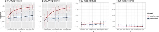
The proportion of the three relevant covariates (i.e., |$X_1, X_2,$| and |$X_3$|⁠) correctly selected (the “true positives”; the two gray panels), and the |$p-3$| irrelevant covariates (i.e., |$X_4, X_5, \ldots, X_p$|⁠) incorrectly selected (the “false positives”; the two white panels), respectively (and |$\pm 1$| standard deviation), as the sample size |$n$| varies from |$100$| to |$1000$|⁠, for each |$p \in \{50, 200\}$|⁠.

Open in new tabDownload slide

4.2. Individualized treatment rule estimation performance

1. The proposed additive regression approach (2.6), estimated via Algorithm 1. The dimension of the basis function |$\boldsymbol{\Psi}_j$| in (3.10) is taken to be |$d_j = 6$||$(j=1,\ldots,p)$|⁠. Given estimates |$\{ \hat{g}_{j}^\ast \}$|⁠, the estimate of |$\mathcal{D}^{\rm opt}$| in (3.19) is |$\hat{\mathcal{D}}^{\rm opt}(\boldsymbol{X}) = \operatorname*{arg\,max}_{a \in \{1,\ldots,L \} } \sum_{j=1}^p \hat{g}_{j,a}^\ast(X_{j})$|⁠.

2. The linear regression (MC) approach (4.21) of Tian and others (2014), implemented through the R-package glmnet, with the sparsity tuning parameter |$\lambda$| selected by minimizing a 10-fold cross-validated prediction error. Given an estimate |$\hat{\boldsymbol{\beta}}^\ast = (\hat{\beta}_1^\ast,\ldots, \hat{\beta}_p^\ast)^\top$|⁠, the corresponding estimate of |$\mathcal{D}^{\rm opt}$| in (3.19) is |$\hat{\mathcal{D}}^{\rm opt}(\boldsymbol{X}) = \operatorname*{arg\,max}_{a \in \{1,\ldots,L \} } \sum_{j=1}^p (a - 1.5 ) X_j \hat{\beta}_j^\ast$|⁠.

3. The OWL method (Zhao and others, 2012) based on a Gaussian radial kernel, implemented in the R-package DTRlearn, with a set of feature transformed (FT) covariates |$\{ \hat{g}_{j,1}^\ast(X_{j}), j=1,\ldots,p \}$| used as an input to the OWL method, in which the functions |$\hat{g}_{j,1}^\ast(\cdot)$||$(j=1,\ldots,p)$| are obtained from the approach in 1. To improve the efficiency of the OWL, we employ the augmented OWL approach of Liu and others (2018). The inverse bandwidth parameter |$\sigma_n^2$| and the tuning parameter |$\kappa$| in Zhao and others (2012) are chosen from the grid of |$(0.01, 0.02, 0.04, \ldots, 0.64, 1.28)$| and that of |$(0.25, 0.5, 1, 2, 4)$| (the default setting of DTRlearn), respectively, based on a |$5$|-fold cross-validation.

4. The same (OWL) approach as in 3 but based on the original features |$\{ X_j, j=1,\ldots,p\}$|⁠.

For each simulation run, we estimate |$\mathcal{D}^{\rm opt}$| from each of the four methods based on a training set (of size |$n \in \{250, 500\}$|⁠), and for evaluation of these methods, we compute the value |$V(\hat{\mathcal{D}}^{\rm opt})$| in (3.18) for each estimate |$\hat{\mathcal{D}}^{\rm opt}$|⁠, using a Monte Carlo approximation based on a random sample of size |$10^3$|⁠. Since we know the true data generating model in simulation studies, the optimal |$\mathcal{D}^{\rm opt}$| can be determined for each simulation run. Given each estimate |$\hat{\mathcal{D}}^{\rm opt}$| of |$\mathcal{D}^{\rm opt}$|⁠, we report |$V(\hat{\mathcal{D}}^{\rm opt}) - V(\mathcal{D}^{\rm opt})$|⁠, as the performance measure of |$\hat{\mathcal{D}}^{\rm opt}$|⁠. A larger value (i.e., a smaller difference from the optimal value) of the measure indicates better performance.

In Figure 2, we present the boxplots, obtained from |$100$| simulation runs, of the normalized values |$V(\hat{\mathcal{D}}^{\rm opt})$| (normalized by the optimal values |$V(\mathcal{D}^{{\rm opt}})$|⁠) of the decision rules |$\hat{\mathcal{D}}^{{\rm opt}}$| estimated from the four approaches, for each combination of |$n \in \{250, 500 \}$|⁠, |$\xi \in \{0, 1\}$| (corresponding to correctly specified or misspecified additive interaction effect models, respectively) and |$\delta \in \{1, 2 \}$| (corresponding to moderate or large main effects, respectively), for the highly nonlinear and moderately nonlinear |$A$|-by-|$\boldsymbol{X}$| interaction effect scenarios, in the top and bottom panels, respectively. The proposed additive regression clearly outperforms the OWL (without feature transformation) method in all scenarios (both the top and bottom panels) and also the linear regression approach in all of the highly nonlinear |$A$|-by-|$\boldsymbol{X}$| interaction effect scenarios (the top panels). For the moderately nonlinear |$A$|-by-|$\boldsymbol{X}$| interaction effect scenarios (the bottom panels), when |$\xi = 0$|⁠, all the methods except the OWL perform at a near-optimal level. On the other hand, when |$\xi = 1$| (i.e., when the underlying |$A$|-by-|$\boldsymbol{X}$| interaction effect model deviates from the additive structure), the more flexible additive model significantly outperforms the linear model. We have also considered a linear |$A$|-by-|$\boldsymbol{X}$| interaction effect case in Section S.5.2 of Supplementary Materials available at Biostatistics online, in which the linear regression outperforms the additive regression, but only slightly, whereas if the underlying model deviates from the exact linear structure and |$n=500$|⁠, the more flexible additive regression tends to outperform the linear model. This suggests that, in the absence of prior knowledge about the form of the interaction effect, employing the proposed additive regression is more suitable for optimizing ITRs than the linear regression. Comparing the two OWL methods (OWL (FT) and OWL), Figure 2 illustrates that the feature transformation based on the estimated component functions |$\{\hat{g}_j^\ast, j=1,\ldots,p \}$| provides a considerable benefit in their performance. This suggests the utility of the proposed model (2.1) as a potential feature transformation and selection tool for a machine learning algorithm for optimizing ITRs. In Figure 2, comparing the cases with |$\delta = 2$| to those with |$\delta = 1$|⁠, the increased magnitude of the main effect generally dampens the performance of all approaches, as the “noise” variability in the data generation model increases.

Figure 2

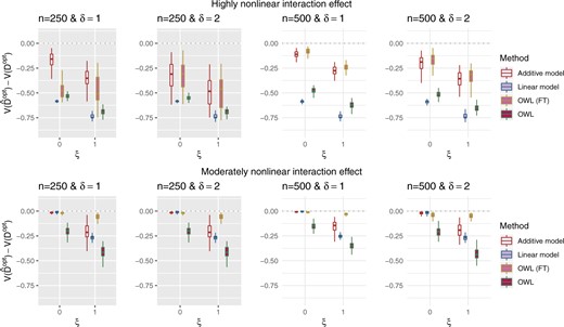
Boxplots based on |$100$| simulation runs, comparing the four approaches to estimating |$\mathcal{D}^{\rm opt}$|⁠, given each scenario indexed by |$\xi \in \{0,1\}$|⁠, |$\delta \in \{1,2\},$| and |$n\in \{250, 500\}$|⁠, for the highly nonlinear |$A$|-by-|$\boldsymbol{X}$| interaction effect case in the top panels, and the moderately nonlinear |$A$|-by-|$\boldsymbol{X}$| interaction effect case in the bottom panels. The dotted horizontal line represents the optimal value corresponding to |$\mathcal{D}^{\rm opt}$|⁠.

Open in new tabDownload slide

5. Application to data from a depression clinical trial

In this section, we illustrate the utility of the proposed additive regression for estimating treatment effect modification and optimizing individualized treatment rules, using data from a depression clinical trial study, comparing an antidepressant and placebo for treating major depressive disorder (Trivedi and others, 2016). The goal of the study is to identify baseline characteristics that are associated with differential response to the antidepressant versus placebo and to use those characteristics to guide treatment decisions when a patient presents for treatment.

Study participants (a total of |$n = 166$| participants) were randomized to either placebo (⁠|$A=1$|⁠; |$n_1 = 88$|⁠) or an antidepressant (sertraline) (⁠|$A=2$|⁠; |$n_2 = 78$|⁠). Subjects were monitored for 8 weeks after initiation of treatment, and the primary endpoint of interest was the Hamilton Rating Scale for Depression (HRSD) score at week 8. The outcome |$Y$| was taken to be the improvement in symptoms severity from baseline to week |$8$|⁠, taken as the difference, i.e., we take: week 0 HRSD score–week 8 HRSD score. (Larger values of the outcome |$Y$| are considered desirable.) The study collected baseline patient clinical data, prior to treatment assignment. These pretreatment clinical data |$\boldsymbol{X} = (X_1, X_2, \ldots, X_{13})^\top \in \mathbb{R}^{13}$| include: |$X_1=$| Age at evaluation; |$X_2=$| Severity of depressive symptoms measured by the HRSD at baseline; |$X_3= $| Logarithm of duration (in month) of the current major depressive episode; and |$X_4=$| Age of onset of the first major depressive episode. In addition to these standard clinical assessments, patients underwent neuropsychiatric testing at baseline to assess psychomotor slowing, working memory, reaction time (RT), and cognitive control (e.g., post-error recovery), as these behavioral characteristics are believed to correspond to biological phenotypes related to response to antidepressants (Petkova and others, 2017) and are considered as potential modifiers of the treatment effect. These neuropsychiatric baseline test measures include: |$X_5=$| (A not B) RT-negative; |$X_6=$| (A not B) RT-non-negative; |$X_{7}= $|(A not B) RT-all; |$X_{8}= $| (A not B) RT-total correct; |$X_9=$| Median choice RT; |$X_{10}=$| Word fluency; |$X_{11}=$| Flanker accuracy; |$X_{12}=$| Flanker RT; |$X_{13}=$| Post-conflict adjustment.

The proposed approach (2.6) to estimating the |$A$|-by-|$\boldsymbol{X}$| interaction effect part |$\sum_{j=1}^p g_{j,A}^\ast(X_j)$| of model (2.1), estimated via Algorithm 1, simultaneously selected |$3$| pretreatment covariates as treatment effect-modifiers: |$X_1$| (“Age at evaluation”), |$X_{10}$| (“Word fluency test”), and |$X_{11}$| (“Flanker accuracy test”). The top panels in Figure 3 illustrate the estimated non-zero component functions |$\{ \hat{g}_j^\ast \ne 0, j=1,\ldots,13 \}$| (i.e., the component functions corresponding to the selected covariates |$X_1$|⁠, |$X_{10}$|⁠, and |$X_{11}$|⁠) and the associated partial residuals. The linear regression approach (4.21) to estimating the |$A$|-by-|$\boldsymbol{X}$| interactions selected a single covariate, |$X_{11}$|⁠, as a treatment effect-modifier.

Figure 3

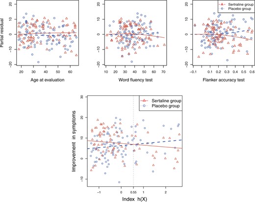
The top panels: Scatterplots of partial residuals vs. the covariates associated with estimated non-zero component functions |$\{ \hat{g}_j^\ast \ne 0 \}$| for placebo (blue circles) and the active drug (red triangles) treated participants; for each panel, the blue dashed curve represents |$\hat{g}_{j,1}^\ast(\cdot)$|⁠, corresponding to the placebo (⁠|$a=1$|⁠), and the red solid curve represents |$\hat{g}_{j,2}^\ast(\cdot)$|⁠, corresponding to the active drug (⁠|$a=2$|⁠). The bottom panel: A scatterplot of the treatment response |$y$| versus the index |$h(\boldsymbol{x}) = \sum_{j=1}^p \hat{g}_{j,1}^\ast(x_j)$|⁠, for the drug (red triangles) and the placebo (blue circles) groups; the blue dashed line is |$y = \hat{\beta}_{0,1} + h(\boldsymbol{x})$| and the red solid line is |$y = \hat{\beta}_{0,2} - \hat{\pi}_2^{-1} \hat{\pi}_1 h(\boldsymbol{x})$|⁠; a gray dashed vertical line indicates the threshold value |$h(\boldsymbol{x})= 0.55$| associated with the ITR |$\hat{\mathcal{D}}^{\rm opt}(\boldsymbol{x})$|⁠.

Open in new tabDownload slide

In this dataset, |$\hat{\beta}_{0,1} = 6.34$| (corresponding to the placebo) and |$\hat{\beta}_{0,2}=7.5$| (corresponding to the drug). The optimal treatment region in the |$X_1, X_{10}, X_{11}$| space, implied by the ITR (5.24), is illustrated in Figure 4, where we have utilized |$40 \times 40 \times 40$| equally spaced grid points (i.e., |$40$| for each axis) for visualization of the regions |$R_1$| and |$R_2$|⁠.

Figure 4

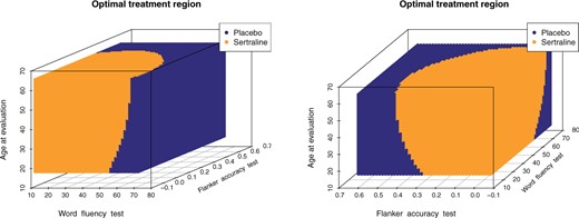
The decision regions |$R_1$| (corresponding to the placebo, dark blue) and |$R_2$| (corresponding to the active drug, orange) displayed in the 3D cube of the three covariates |$X_1$| (age at evaluation), |$X_{10}$| (word fluency test), and |$X_{11}$| (Flanker accuracy test), evaluated at |$40 \times 40 \times 40$| equally spaced grid points (⁠|$40$| for each axis), shown from two different angles (left and right panels).

Open in new tabDownload slide

For an alternative way of visualizing the ITR (5.24), let us define a 1D index |$h(\boldsymbol{X}) = \sum_{j=1}^p \hat{g}_{j,1}^\ast(X_j)$|⁠. By the constraint (2.2), we have the relationship |$\sum_{j=1}^p \hat{g}_{j,2}^\ast(X_j) = - \hat{\pi}_2^{-1} \hat{\pi}_1 \big\{ \sum_{j=1}^p \hat{g}_{j,1}^\ast(X_j) \big\}$|⁠. Therefore, the term |$\sum_{j=1}^p \big\{ \hat{g}_{j,2}^\ast(X_j) - \hat{g}_{j,1}^\ast(X_j) \big\}$| in the decision rule (5.24) can be reparametrized, with respect to |$h(\boldsymbol{X})$|⁠, as |$(- \hat{\pi}_2^{-1} \hat{\pi}_1 - 1) h(\boldsymbol{X})$|⁠. In this dataset, |$\hat{\pi}_1 = 0.53$| and |$\hat{\pi}_2 = 0.47$|⁠, and thus the ITR (5.24) can be re-written as: |$\hat{\mathcal{D}}^{\rm opt}(\boldsymbol{X}) = I\big[ 1.16 -2.12 h(\boldsymbol{X}) > 0 \big] + 1;$| this ITR indicates that, for a patient with pretreatment characteristics |$\boldsymbol{x}$|⁠, if |$h(\boldsymbol{x}) < 0.55 \ (\approx 1.16/2.12)$|⁠, then he/she would be recommended the active drug (⁠|$a=2$|⁠) and the placebo (⁠|$a=1$|⁠), otherwise. For example, for a patient with |$x_1= 40$|⁠, |$x_{10} = 50,$| and |$x_{11} = 0.4$|⁠, the index |$h(\boldsymbol{x}) = 1.01 > 0.55$| (see the bottom panel in Figure 3 for a visualization) and thus the patient would be recommended the placebo.

To evaluate the performance of the ITRs (⁠|$\hat{\mathcal{D}}^{{\rm opt}}$|⁠) obtained from the four different approaches described in Section 4.2, we randomly split the data into a training set and a testing set (of size |$\tilde{n})$| using a ratio of |$5$| to |$1$|⁠, replicated |$500$| times, each time computing an ITR |$\hat{\mathcal{D}}^{{\rm opt}}$| based on the training set, then estimating its value |$V(\hat{\mathcal{D}}^{{\rm opt}})$| in (3.18) by an inverse probability weighted estimator (Murphy, 2005): |$\hat{V}(\hat{\mathcal{D}}^{{\rm opt}}) = \sum_{i=1}^{\tilde{n}} Y_{i} I_{(A_i = \hat{\mathcal{D}}^{{\rm opt}}(\boldsymbol{X}_i) )} / \sum_{i=1}^{\tilde{n}} I_{(A_i =\hat{\mathcal{D}}^{{\rm opt}}(\boldsymbol{X}_i)) }$|⁠, computed based on the testing set of size |$\tilde{n}$|⁠. For comparison, we also include two naïve rules: treating all patients with placebo (“All PBO”) and treating all patients with the active drug (“All DRUG”), each regardless of the individual patient’s characteristics |$\boldsymbol{X}$|⁠. The resulting boxplots obtained from the |$500$| random splits are illustrated in Figure 5. A larger value of the measure indicates better performance.

Figure 5

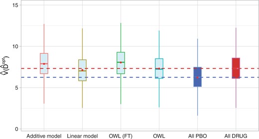
Boxplots of the estimated values of the treatment rules |$\hat{\mathcal{D}}^{\rm opt}$| estimated from |$6$| approaches, obtained from |$500$| randomly split testing sets. Higher values are preferred.

Open in new tabDownload slide

The results in Figure 5 demonstrate that the proposed additive regression approach, which allows nonlinear flexibility in developing ITRs, tends to outperform the linear regression approach, in terms of the estimated value. The additive regression approach also shows some superiority over the method OWL (without feature transformation). In comparison to the OWL methods, the proposed additive regression, in addition to its superior computational efficiency, provides a means of simultaneously selecting treatment effect-modifiers and allows a visualization for the heterogeneous effects attributable to each estimated treatment effect-modifier as in Figure 3, which is an appealing feature in practice. Moreover, the estimated component functions |$\{\hat{g}_j^\ast, j=1,\ldots,p\}$| of the proposed regression provide an effective means of performing feature transformation for |$\{X_j, j=1,\ldots,p\}$|⁠. As in Section 4.2, the FT OWL approach appears to have a considerable improvement over the OWL that bases on the original untransformed covariates.

6. Discussion

In this article, we have developed a sparse additive model, via a structural constraint, specifically geared to identify and model treatment effect-modifiers. The approach utilizes an efficient back-fitting algorithm for model estimation and variable selection. The proposed sparse additive model for treatment effect modification extends existing linear model-based regression methods by providing nonlinear flexibility to modeling treatment-by-covariate interactions. Encouraged by our simulation results and the application, future work will investigate the asymptotic properties related to treatment effect-modifier selection and estimation consistency, in addition to developing hypothesis testing procedures for treatment-by-covariates interaction effects.

Modern advances in biotechnology, using measures of brain structure and function obtained from neuroimaging modalities (e.g., magnetic resonance imaging (MRI), functional MRI, and electroencephalography), show the promise of discovering potential biomarkers for heterogeneous treatment effects. These high-dimensional data modalities are often in the form of curves or images and can be viewed as functional data (e.g., Ramsay and Silverman, 1997). Future work will also extend the additive model approach to the context of functional additive regression (e.g., Fan and others, 2014, 2015). The goal of these extensions will be to handle a large number of functional-valued covariates while achieving simultaneous variable selection, which will extend current functional linear model-based methods for precision medicine (McKeague and Qian, 2014; Ciarleglio and others, 2015; 2018) to a more flexible functional regression setting, as well as to longitudinally observed functional data (e.g., Park and Lee 2019).

7. Software

R-package samTEMsel (Sparse Additive Models for Treatment Effect-Modifier Selection) contains R-codes to perform the methods proposed in the article, and is publicly available on GitHub (github.com/syhyunpark/samTEMsel).

Supplementary material

Supplementary material is available at http://biostatistics.oxfordjournals.org

Funding

National Institute of Mental Health (NIMH) (5 R01 MH099003).

Acknowledgments

We are grateful to the editors, the associate editor, and two referees for their insightful comments and suggestions. Conflict of Interest: None declared.

References