


Summary
Divide-and-conquer (DAC) is a commonly used strategy to overcome the challenges of extraordinarily large data, by first breaking the dataset into series of data blocks, then combining results from individual data blocks to obtain a final estimation. Various DAC algorithms have been proposed to fit a sparse predictive regression model in the |$L_1$| regularization setting. However, many existing DAC algorithms remain computationally intensive when sample size and number of candidate predictors are both large. In addition, no existing DAC procedures provide inference for quantifying the accuracy of risk prediction models. In this article, we propose a screening and one-step linearization infused DAC (SOLID) algorithm to fit sparse logistic regression to massive datasets, by integrating the DAC strategy with a screening step and sequences of linearization. This enables us to maximize the likelihood with only selected covariates and perform penalized estimation via a fast approximation to the likelihood. To assess the accuracy of a predictive regression model, we develop a modified cross-validation (MCV) that utilizes the side products of the SOLID, substantially reducing the computational burden. Compared with existing DAC methods, the MCV procedure is the first to make inference on accuracy. Extensive simulation studies suggest that the proposed SOLID and MCV procedures substantially outperform the existing methods with respect to computational speed and achieve similar statistical efficiency as the full sample-based estimator. We also demonstrate that the proposed inference procedure provides valid interval estimators. We apply the proposed SOLID procedure to develop and validate a classification model for disease diagnosis using narrative clinical notes based on electronic medical record data from Partners HealthCare.
1. Introduction
Large-scale healthcare data, including those from electronic medical records (EMR) and insurance claims data, open tremendous opportunities for novel discoveries. For example, risk prediction models can be developed using EMR data and incorporated into the healthcare system as clinical decision support. However, developing risk prediction models using massive and rich datasets is computationally challenging since often times both the sample size, |$n_0$|, and the number of candidate predictors, |$p$|, are large. To develop an accurate yet clinically interpretable risk model in such a high dimensional setting, we may fit regularized regression procedures with various penalties that can simultaneously remove non-informative predictors and estimate the effects of the informative predictors Tibshirani, 1996; Fan and Li, 2001; Zou and Hastie, 2005; Zou, 2006, e.g.). However, when |$n_0$| is extraordinarily large, directly fitting a sparse predictive model is not computationally feasible.
One strategy to overcome the computational difficulty is to employ a divide-and-conquer (DAC) scheme. Standard DAC procedures divide the full sample into |$K$| subsets, solve the optimization problem using each subset, and then combine subset-specific estimates to form a final DAC estimate. A wide range of DAC algorithms have been proposed to fit various prediction models, but we will only focus our discussion on |$L_1$|-type penalized regression due to its advantage in interpretability. Chen and Xie (2014) proposed a DAC algorithm to fit penalized GLM. The algorithm obtains a sparse GLM estimate for each subset and then combines subset-specific estimates by majority voting and averaging. Wang and others (2014) proposed a median selection subset aggregation estimator by first fitting |$L_1$| penalized linear regression in each data block to select informative features, and then performing a DAC linear regression with only selected features. Lee and others (2017) proposed a one-shot de-biased lasso approach, by obtaining the de-biased lasso estimate (Van de Geer and others, 2014) at each data block, then simply averaging the local de-biased lasso estimates. Tang and others (2016) also obtained the same de-biased lasso estimate of each data block, but then used a robust meta-analysis-type approach through the confidence distribution approach (Xie and others, 2011) to combine the local estimates. He and others (2016) propose a sparse meta-analysis approach to integrate information across sites for the low-dimensional setting with small |$p$|. While the above algorithms are effective in reducing the computational burden compared to fitting a penalized regression model to the full data, they remain computationally intensive as they require |$K$| penalized estimation procedures. It is of great interest to further reduce the computational burden when fitting extraordinarily large data. Recently, building on the work of Wang and Leng (2007), Wang and others (2019) proposed an efficient DAC algorithm to fit sparse Cox regression by using a one-step linear approximation followed by a least square approximation (LSA) without requiring fitting penalized Cox model on all |$K$| sets. Although this approach can be adapted for logistic regression, it is not computationally efficient when |$p$| is large.
After a risk prediction model is developed, a critical follow-up step is to evaluate its prediction performance in order to determine whether it is feasible to adopt in practice. A wide range of accuracy parameters such as the receiving operating characteristic (ROC) curve have been proposed as performance measures (Pepe, 2003). Making inference about the accuracy parameters with an exceedingly large dataset is also computationally challenging, especially if the accuracy estimators are non-smooth functionals. Under standard settings with moderate |$n_0$| and |$p$|, to make inference about the prediction accuracy of a fitted model, cross-validation (CV) is often used to correct overfitting bias and resampling methods are used for variance estimation (Tian and others, 2007; Uno and others, 2007, e.g.). Both CV and resampling becomes computationally infeasible for exceedingly large datasets.
In this article, we propose a screening and one-step linearization infused DAC (SOLID) procedure for efficiently estimating a sparse prediction model. The SOLID procedure attains computational and statistical efficiency by integrating DAC with an initial screening for an active set of estimators, and sequences of one-step linear approximation. The main advantage of the SOLID procedure compared with existing DAC procedures is that it substantially increases the computational efficiency when |$n_0$| and |$p$| are both large. To efficiently make inference about the accuracy of the prediction model, we develop a modified cross-validation (MCV), which achieves the same asymptotic efficiency as the standard CV. The MCV procedure directly utilizes side products from the SOLID procedure to estimate the corresponding accuracy parameters without additionally applying the full SOLID procedure in each random split, but still adjusting for overfitting. Specifically, during the SOLID procedure, summary statistics such as score function and hessian matrix are obtained for each data block. At the |$k$|th fold for a |$K$|-fold MCV, instead of applying the full SOLID procedure to |$K-1$| data blocks (taking out the |$k$|th data block), the model estimation is approximated by combining summary statistics of |$K-1$| data blocks which are already available. To the best of our knowledge, the proposed MCV procedure is the first effort to make inference on accuracy and adjust for overfitting under the DAC framework.
The rest of the article is organized as follows. In Section 2, we detail the SOLID procedure and the MCV. We also propose the efficient standard error estimation for the non-smooth function. In Section 3, we present simulation results demonstrating the superiority of the proposed methods compared to the existing methods. In Section 4, we employ the SOLID and the MCV to Partners HealthCare EMR data to assign ICD codes of depression to patient visits. We conclude with discussions in Section 5.
2. Methods
2.1. Notations and settings
Let |$Y$| denote the binary outcome, and |${\bf X}$| denote the |$(p+1)\times 1$| vector of predictors, where we include 1 as the first element of |${\bf X}$|. Suppose the full data consist of |$n_0$| independent and identically distributed realizations of |${\bf D} = (Y,{\bf X}^{{\sf \scriptscriptstyle{T}}})^{{\sf \scriptscriptstyle{T}}}$|, denoted by |$\mathscr{D}_{\sf \scriptscriptstyle +} = \{{\bf D}_i, i = 1,..., n_0\}$|. We denote the index set for the full data by |$\Omega_{\sf \scriptscriptstyle +} = \{1,..., n_0\}$|. We randomly partition |$\mathscr{D}_{\sf \scriptscriptstyle +}$| into |$K$| subsets with the |$k$|th subset denoted by |$\mathscr{D}_k = \{{\bf D}_i, i \in \Omega_k\}$|. Without loss of generality, we assume that |$n = n_0/K$| is an integer and that the index set for the subset |$k$| is |$\Omega_k = \{(k-1)n+1,..., kn\}$|. For any index set |$\Omega$|, we denote the size of |$\Omega$| by |$n_{\Omega}$| with |$n_{\Omega}=n_0$| if |$\Omega=\Omega_{\sf \scriptscriptstyle +}$| and |$n_{\Omega}=n$| if |$\Omega=\Omega_k$|.
The oracle property holds when the asymptotic distribution of the estimator is the same as the asymptotic distribution of the MLE on the true support. When |$n_0$| is exceedingly large, obtaining |$\widehat{\boldsymbol{\beta}}_{\scriptscriptstyle\Omega_{\sf \scriptscriptstyle +}}$| is not computationally feasible. Our first goal is to employ SOLID to obtain a computationally efficient estimator that achieves the same efficiency as the full sample estimator |$\widehat{\boldsymbol{\beta}}_{\scriptscriptstyle\Omega_{\sf \scriptscriptstyle +}}$|.
One may summarize the trade-off between the TPR and FPR functions based on the ROC curve, |$\text{ROC}(u)=\text{TPR}\left\{\text{FPR}^{-1}(u)\right\}.$| Additionally, the area under the ROC curve |$\text{AUC}=\int_0^1 \text{ROC}(u){\rm d}u$|, summarizes the overall prediction performance of |$\pi_{\scriptscriptstyle \widehat{\boldsymbol{\beta}}}^{\sf \scriptscriptstyle{new}}$|. With a selected threshold |$c$|, it is also often desirable to evaluate the positive predictive value (PPV) and negative predictive value (NPV) of the binary rule |$I(\pi_{\scriptscriptstyle \widehat{\boldsymbol{\beta}}}^{\sf \scriptscriptstyle{new}}\ge c)$| defined as |$\text{PPV}(c)=E\{\text{PPV}(c; \widehat{\boldsymbol{\beta}})\}$| and |$\text{NPV}(c)=E\{\text{NPV}(c; \widehat{\boldsymbol{\beta}})\}$|, where |$\text{PPV}(c; \boldsymbol{\beta}) = P(Y=1|\pi_{\scriptscriptstyle \boldsymbol{\beta}}^{\sf \scriptscriptstyle{new}} \ge c)$| and |$\text{NPV}(c; \boldsymbol{\beta})=P(Y^{\sf \scriptscriptstyle{new}}=0|\pi_{\scriptscriptstyle \boldsymbol{\beta}}^{\sf \scriptscriptstyle{new}}< c).$| For simplicity, we will use |$\text{TPR}(c)$| to illustrate the proposed method in this section but note that estimation procedures can be similarly formed for other accuracy measures. We propose an efficient MCV procedure to construct bias corrected point and interval estimators for |$\text{TPR}$|.
2.2. SOLID algorithm for approximating |$\widehat{\boldsymbol{\beta}}_{\scriptscriptstyle\Omega_{\sf \scriptscriptstyle +}}$|
Following similar arguments given in Caner and Zhang (2014), one may show that |$\widehat{\boldsymbol{\beta}}_{\scriptscriptstyle\Omega_{\sf \scriptscriptstyle +}}^{\sf\scriptscriptstyle lin}$| will also achieve the variable selection consistency as |$\widehat{\boldsymbol{\beta}}_{\scriptscriptstyle\Omega_{\sf \scriptscriptstyle +}}$| and that |$\widehat{\boldsymbol{\beta}}_{\scriptscriptstyle\Omega_{\sf \scriptscriptstyle +}}^{\sf\scriptscriptstyle lin}Asc$| has the same limiting distribution as that of |$\widehat{\boldsymbol{\beta}}_{\scriptscriptstyle\Omega_{\sf \scriptscriptstyle +}}^{\scriptscriptstyle{{\cal A}}}$|. This suggests that an estimator can recover the distribution of |$\widehat{\boldsymbol{\beta}}_{\scriptscriptstyle\Omega_{\sf \scriptscriptstyle +}}$| if we can construct an accurate DAC approximations to |$\widetilde{\boldsymbol{\beta}}_{\Omega_{\sf \scriptscriptstyle +}}$| and |$\widehat{\mathbb{A}}_{\Omega_{\sf \scriptscriptstyle +}}(\widetilde{\boldsymbol{\beta}}_{\Omega_{\sf \scriptscriptstyle +}})$|. To this end, we propose the SOLID procedure, which requires two main steps: (i) screening for an active set of predictors; (ii) constructing a linearized adaptive LASSO estimator with the active set. In both steps, linearization via the LSA are used.
The screening step consists of four sub-steps:
The post-screening linearized adaptive LASSO fitting step consists of two main sub-steps:
The SOLID estimator will always take value 0 for the elements that are deemed 0 in the screening step and only requires estimation of |$\boldsymbol{\beta}$| for the elements in |$\widehat{{\cal A}}$|. The linearization in step (2.2) allows us to solve the penalized regression step using a pseudo likelihood based on a size of |$\mbox{Card}(\widehat{{\cal A}})$| data points, which is substantially smaller than the original sample size |$n$| in likelihood of each subset. Compared to solving (2.2), the computation cost of SOLID is substantially lower when |$n_0\gg p$| and |$p$| is also not small.
Following similar arguments as given in Wang and others (2019), Zou and Zhang (2009), and Cui and others (2017), one may show that the proposed SOLID estimator attains the same oracle properties as those of |$\widehat{\boldsymbol{\beta}}_{\scriptscriptstyle\Omega_{\sf \scriptscriptstyle +}}$| under the same regularity conditions given in Zou and Zhang (2009) provided that |$K = o\left(n^{\frac{1}{2}}_0\right)$|. In the screening step, the one-step estimator |$\widetilde{\boldsymbol{\beta}}_{\Omega_{\sf \scriptscriptstyle +}}^{\sf\scriptscriptstyle lin,1}$| has a convergence rate of |$\|\widetilde{\boldsymbol{\beta}}_{\Omega_{\sf \scriptscriptstyle +}}^{\sf\scriptscriptstyle lin,1}-\boldsymbol{\beta}_0\|_{\infty} = O_p\{p/n_{\Omega_1}+\sqrt{\log(p)/n_0}\}$|, which is slower than that of |$\|\widetilde{\boldsymbol{\beta}}_{\Omega_{\sf \scriptscriptstyle +}}-\boldsymbol{\beta}_0\|_{\infty}=O_p\{\sqrt{\log(p)/n_0}\}$| when |$d_1\equiv\lim_{n_0\to \infty} \log(n_{\Omega_1})/\log(n_0) < (1+\nu)/2$|. Nevertheless, when |$\lambda_{\sf\scriptscriptstyle screen} =O\{(n_0^{-1/2}+p/n_{\Omega_1})^{(1-\nu)(1+\gamma)}\}$|, we may follow similar arguments as given in Zou and Zhang (2009) to show that |$P(\widehat{{\cal A}}=\mathcal{A}) \to 1$| as |$n_0\to \infty$| and |$\|\widehat{\boldsymbol{\beta}}_{\sf\scriptscriptstyle screen}^{\scriptscriptstyle{{\cal A}}}sc - \boldsymbol{\beta}_0^{\scriptscriptstyle{{\cal A}}}sc\|_2 = O_p(p/n_{\Omega_1}+n_0^{-1/2})$|. In addition, when |$M$| is sufficiently large, |$\widehat{\cal A}_{\sf \scriptscriptstyle{SOLID}}$| attains the oracle properties in that |$P(\widehat{\cal A}_{\sf \scriptscriptstyle{SOLID}}={\cal A})\rightarrow1$| and |$\sqrt{n_0}(\widehat{\boldsymbol{\beta}}_{\sf \scriptscriptstyle{SOLID},j}^{\scriptscriptstyle{{\cal A}}}sc - \boldsymbol{\beta}_0^{\scriptscriptstyle{{\cal A}}}sc)$| and |$\sqrt{n_0}(\widehat{\boldsymbol{\beta}}_{\scriptscriptstyle\Omega_{\sf \scriptscriptstyle +}}^{\mathcal{A}}- \boldsymbol{\beta}_0^{\scriptscriptstyle{{\cal A}}}sc)$| have the same limiting distribution, where |$\widehat{{\cal A}}_{\sf \scriptscriptstyle{SOLID},j} = \{j: \widehat{\boldsymbol{\beta}}_{\sf \scriptscriptstyle{SOLID},j}/{\hspace{-3.5mm}} = 0\} \supseteq \widehat{{\cal A}}$|.
We use the ridge estimator in (1.1) instead of the standard MLE since |$n_{\Omega_1}$| may not be substantially larger than |$p$|, in which case the ridge estimator is more stable than MLE. In practice, we find that both MLE and the ridge estimator work well when |$p \ll n_{\Omega_1}$| (e.g., |$p=50$| and |$n_{\Omega_1} = 10^4$|), but the ridge estimator is much more stable otherwise (e.g., |$p=500$| and |$n_{\Omega_1} = 10^4$|).
Although theoretically |$\widehat{{\cal A}}$| from the screening step can already consistently estimate |$\mathcal{A}$|, we follow-up with a refined estimate in (2.1) and (2.2) since |$\widehat{{\cal A}}$| is obtained based on the one-step estimator |$\widetilde{\boldsymbol{\beta}}_{\Omega_{\sf \scriptscriptstyle +}}^{\sf\scriptscriptstyle lin,1}$| which has a sub-optimal convergence rate. In practice, one may also choose a slightly conservative |$\lambda_{\sf\scriptscriptstyle screen}$| to make sure that the screening step will not remove any true signals.
Step (2.1) requires |$M$| iterations and can be done relatively fast since it is constraining to the subset identified by |$\widehat{{\cal A}}$| which is substantially smaller than |$p$|. In practice, one may find |$M$| such that step (2.1) converges or to ensure |$(p/n_{\Omega_1}+n_0^{-1/2})^{2^M} = o( n_0^{-1/2})$|, i.e., |$M > \log\{1/(d_1-\nu)\}/\log(2)-1$| if |$p = c \times n_0^{\nu}$| and |$n_{\Omega_1} = c \times n_0^{d_1}$| for some constant |$c$|. When either holds, |$\widetilde{\boldsymbol{\beta}}_{\sf \scriptscriptstyle{DAC}}^{\scriptscriptstyle{{\cal A}}}sc$| is asymptotically equivalent to the solution to |$\widehat{{\bf U}}_{\sf \scriptscriptstyle{DAC}}^{\scriptscriptstyle{{\cal A}}}sc(\boldsymbol{\beta}^{\scriptscriptstyle{{\cal A}}}sc) = {\bf 0}$|.
2.3. Modified cross-validation for model evaluation
We obtain |$\widehat{\boldsymbol{\beta}}^{\scriptscriptstyle \widehat{\mathcal{A}}} _{{\sf \scriptscriptstyle{DAC}},{\sf \scriptscriptstyle{-k}}}$| by repeating steps 1.2 to 2.2 of the SOLID procedure but taking out the |$k$|th data block as follows:
We obtain the active set |$\widehat{\cal A}_{-k}= \{\jmath: \widehat{\boldsymbol{\beta}}_{\sf\scriptscriptstyle screen,-k} \ne 0\}.$|
Let |$\widetilde{\boldsymbol{\beta}}_{{\sf \scriptscriptstyle{DAC}},{\sf \scriptscriptstyle{-k}}}^{\scriptscriptstyle \widehat{\mathcal{A}}}=\widetilde{\boldsymbol{\beta}}_{{\sf \scriptscriptstyle{DAC}},{\sf \scriptscriptstyle{-k}}}^{[M]}$|.
It is worth mentioning that the major time cost of the SOLID procedure lies in the calculation of |$\widetilde{\boldsymbol{\beta}}_{\Omega_1}^{\sf \scriptscriptstyle rid}$| in step (1.1) and the calculation of |$\widehat{{\bf U}}_{\Omega_{k}}$| and |$\widehat{\mathbb{A}}_{\Omega_k}$| for |$k=1, \ldots, K$| in step (1.2). In the MCV procedure, we reuse |$\widetilde{\boldsymbol{\beta}}_{\Omega_1}^{\sf \scriptscriptstyle rid}$|, |$\widehat{{\bf U}}_{\Omega_{k}}$|, and |$\widehat{\mathbb{A}}_{\Omega_k}$| as the side products from the SOLID procedure, thereby substantially reducing the time cost.
2.4. Tuning and standard errors calculation
3. Simulations
3.1. Simulation settings
We generate |${\bf X}_{-1}$| from |$N(\textbf{0}_p^{{\sf \scriptscriptstyle{T}}}, \mathbb{V})$| with |$\mathbb{V}=0.8\mathbb{I}_{p\times p} + 0.2$|, where |$\mathbb{I}$| is the identity matrix.
For model estimation, we compare the SOLID estimator with four existing estimators: (i) the full sample-based adaptive lasso estimator |$\widehat{\boldsymbol{\beta}}_{\scriptscriptstyle\Omega_{\sf \scriptscriptstyle +}}$|; (ii) the majority voting-based DAC scheme for GLM proposed by Chen and Xie (2014), denoted by |$\widehat{\boldsymbol{\beta}}_{\scriptscriptstyle \sf Chen}$|; (iii) the de-biased LASSO-based DAC scheme for GLM proposed by Tang and others (2016), denoted by |$\widehat{\boldsymbol{\beta}}_{\scriptscriptstyle \sf Tang}$|; (iv) the sparse meta-analysis approach |$\widehat{\boldsymbol{\beta}}_{\scriptscriptstyle \sf SMA}$| proposed by He and others (2016), denoted by |$\widehat{\boldsymbol{\beta}}_{\scriptscriptstyle \sf SMA}$|. For all methods except for SMA, we set |$\gamma=1$| for fair comparison. When implementing SMA, we set |$\gamma =0$| so that no initial estimator is needed for the procedure due to the high computational cost of the SMA procedure. For model evaluation, we compare the MCV estimator with the external estimator (EXT), which is obtained by evaluating the proposed models on a large external validation size of |$10^6$|. We also compare the MCV estimator with the apparent estimator (APP).
For any |$\widehat{\boldsymbol{\beta}}\in\{\widehat{\boldsymbol{\beta}}_{\sf \scriptscriptstyle{DAC}}, \widehat{\boldsymbol{\beta}}_{\scriptscriptstyle\Omega_{\sf \scriptscriptstyle +}}, \widehat{\boldsymbol{\beta}}_{\scriptscriptstyle \sf Chen}, \widehat{\boldsymbol{\beta}}_{\scriptscriptstyle \sf Tang}, \widehat{\boldsymbol{\beta}}_{\scriptscriptstyle \sf SMA}\}$|, we report (i) the average computation time for |$\widehat{\boldsymbol{\beta}}$|; (ii) the global mean squared error (GMSE), defined as |$(\widehat{\boldsymbol{\beta}} - \boldsymbol{\beta}_0)^{{\sf \scriptscriptstyle{T}}}\mathbb{V}(\widehat{\boldsymbol{\beta}}-\boldsymbol{\beta}_0)$|; (iii) the bias of each individual coefficient; (iv) mean squared error (MSE) of each individual coefficient; (v) empirical probability of |$\jmath\not\in\widehat{{\cal A}}$|; (vi) the empirical coverage level of the 95% normal confidence interval (CI). For model evaluation comparison, we report (i) the average computation time for calculating the ROC curve using EXT, APP and MCV; (ii) the average difference (DIFF) between APP and EXT accuracy estimates, and that between MCV and EXT accuracy estimates; (iii) the empirical standard errors of the EXT, APP, and MCV accuracy estimates; (iv) the average approximated standard error (ASE) of the MCV accuracy estimate as derived in equation (2.7); (v) the coverage level of the 95% normal confidence interval of APP and MCV estimates. Taking TPR for example, we defined “coverage” as the proportion of times that the confidence interval of |$\widehat{\text{TPR}}_{\sf \scriptscriptstyle{APP}}$| or |$\widehat{\text{TPR}}_{\sf \scriptscriptstyle{MCV}}$| contains |$\overline{\text{TPR}}_{\sf \scriptscriptstyle{EXT}}$|, where |$\overline{\text{TPR}}_{\sf \scriptscriptstyle{EXT}}$| is defined as the average of |$\widehat{\text{TPR}}_{\sf \scriptscriptstyle{EXT}}$| taken over both the repeated sample and |$\widehat{\boldsymbol{\beta}}_{\sf \scriptscriptstyle{SOLID},j}$| of 1000 simulations. Note that |$\overline{\text{TPR}}_{\sf \scriptscriptstyle{EXT}}(c)$| is essentially a Monte Carlo estimator of the population parameter |$\text{TPR}(c) = E\{\text{TPR}(c; \widehat{\boldsymbol{\beta}})\}$|, where |$\text{TPR}(c; \boldsymbol{\beta}) = P(\pi_{\scriptscriptstyle \boldsymbol{\beta}}^{\sf \scriptscriptstyle{new}} > c \mid Y^{\sf \scriptscriptstyle{new}} = 1) $|.
The statistical performance is evaluated based on 1000 simulated datasets for each setting. Each simulation is performed on one core at a cluster with Intel ® Xeon® E5-2697 v3 @2.60GHz.
3.2. Simulation results
We first conduct sensitivity studies of the number of iterations |$M$| to examine the impact of |$M$| on the proposed estimator |$\widehat{\boldsymbol{\beta}}_{\sf \scriptscriptstyle{SOLID},j}$|. Across all settings, we found that it is suffices to let |$M=3$| for |$p \le 500$| and |$M=6$| for |$p=1000$|. Hence we summarize below the results for |$\widehat{\boldsymbol{\beta}}_{\sf \scriptscriptstyle{SOLID},j}$| with |$M=3$| for |$p=50$| and |$500$|, and |$M=6$| for |$p=1000$| unless noted otherwise. These choices ensure that |$M > \log\{1/(d_1-\nu)\}/\log(2)-1$| as required by the theoretical results.
We summarize in Table 1 the performance measures of different regression estimators for settings I–III, and in the Supplementary Materials available at Biostatistics online the performance for setting IV. There are substantial differences in computation time across methods and the proposed SOLID algorithm is significantly faster than all competing DAC methods. The relative performance with respect to computation time is similar across the three sets of |$\boldsymbol{\beta}$| but gains in computational efficiency are even larger for larger |$p$|. For example when |$p = 1000$|, the SOLID algorithm is at least 10 times faster than competing DAC methods.
Comparisons among the proposed SOLID algorithm, the standard adaptive LASSO (Full), the sparse meta-analysis approach (SMA), the algorithms proposed by Tang and Chen in regards to averaged computing time in minutes, global mean square error (GMSE)|$\times 10^5$|, bias |$\times 10^3$|, and coverage probability (CP) |$\times 10^2$| of each individual coefficient. For individual |$\beta_j$|’s, we only present the results for the six unique values with |$(b_1, b_2, b_3,b_4,b_5,b_6)$| taking values |$(1,0.8,0.4,0.2,0.1,0)$| in (I) and (II) and |$(0.5,0.4,0.2,0.1,0.05,0)$| in (III).
| Bias | CP | ||||||||||||||
|---|---|---|---|---|---|---|---|---|---|---|---|---|---|---|---|
| p | Method | Time | GMSE | |$b_1$| | |$b_2$| | |$b_3$| | |$b_4$| | |$b_5$| | |$b_6$| | |$b_1$| | |$b_2$| | |$b_3$| | |$b_4$| | |$b_5$| | |
| I | 50 | FULL | 8.97 | 5.11 | 2.78 | 2.63 | 2.50 | 2.51 | 2.72 | 0.00 | 94.0 | 94.3 | 95.2 | 95.0 | 93.2 |
| SOLID | 0.06 | 5.54 | 3.02 | 2.74 | 2.53 | 2.51 | 2.59 | 0.00 | 95.6 | 95.6 | 94.9 | 95.3 | 95.7 | ||
| SMA | 0.24 | 156 | 15.9 | 14.2 | 8.74 | 7.43 | 5.10 | 1.25 | 0.0 | 0.0 | 22.7 | 56.8 | 63.6 | ||
| Tang | 7.01 | 44.2 | 3.18 | 3.06 | 2.69 | 2.60 | 2.71 | 2.57 | 93.7 | 93.9 | 94.6 | 95.3 | 94.7 | ||
| Chen | 7.01 | 5.93 | 3.07 | 2.96 | 2.55 | 2.48 | 2.61 | 0.00 | 93.3 | 93.0 | 94.9 | 94.9 | 94.9 | ||
| 500 | FULL | 103 | 5.42 | 2.83 | 2.87 | 2.51 | 2.58 | 2.63 | 0.00 | 95.1 | 95.3 | 94.8 | 94.7 | 94.3 | |
| SOLID | 1.66 | 5.33 | 2.78 | 2.66 | 2.51 | 2.54 | 2.61 | 0.00 | 94.6 | 95.6 | 94.3 | 94.5 | 92.5 | ||
| SMA | 21.8 | 2927 | 91.1 | 74.3 | 40.3 | 23.7 | 15.6 | 0.07 | 0.0 | 0.0 | 0.0 | 0.0 | 0.0 | ||
| Tang | 94.0 | 429 | 3.01 | 2.98 | 2.76 | 2.65 | 2.71 | 2.58 | 93.1 | 95.0 | 94.3 | 94.5 | 94.8 | ||
| Chen | 92.9 | 5.60 | 2.90 | 2.81 | 2.58 | 2.55 | 2.54 | 0.00 | 93.1 | 94.8 | 93.5 | 94.3 | 94.8 | ||
| 1000 | FULL | 539 | 5.11 | 2.87 | 2.73 | 2.30 | 2.32 | 2.39 | 0.00 | 87.6 | 88.0 | 96.8 | 92.2 | 94.0 | |
| SOLID | 9.41 | 5.53 | 2.89 | 2.73 | 2.64 | 2.70 | 2.71 | 0.00 | 94.2 | 94.2 | 93.4 | 95.0 | 94.2 | ||
| SMA | 100 | 10365 | 180 | 145 | 77.0 | 42.8 | 25.6 | 0.01 | 0.0 | 0.0 | 0.0 | 0.0 | 0.0 | ||
| Tang | 200 | 862 | 3.12 | 2.90 | 2.64 | 2.47 | 2.48 | 2.50 | 93.7 | 94.2 | 95.5 | 95.3 | 95.8 | ||
| Chen | 206 | 5.34 | 3.01 | 2.77 | 2.53 | 2.37 | 2.36 | 0.00 | 94.7 | 92.6 | 94.5 | 94.7 | 95.0 | ||
| II | 50 | FULL | 9.41 | 12.8 | 3.30 | 2.79 | 2.79 | 2.86 | 2.79 | 0.00 | 96.0 | 94.4 | 94.8 | 95.1 | 93.9 |
| SOLID | 0.06 | 13.0 | 3.14 | 2.99 | 2.98 | 2.70 | 2.80 | 0.00 | 95.1 | 95.2 | 94.9 | 95.0 | 94.8 | ||
| SMA | 0.33 | 80.4 | 9.01 | 7.32 | 4.14 | 3.22 | 3.04 | 0.00 | 33.6 | 51.3 | 84.0 | 91.8 | 90.3 | ||
| Tang | 7.08 | 59.1 | 3.90 | 3.56 | 2.91 | 2.88 | 2.88 | 2.75 | 88.9 | 91.2 | 93.9 | 94.9 | 95.6 | ||
| Chen | 7.06 | 18.8 | 3.86 | 3.52 | 2.89 | 2.81 | 2.79 | 0.00 | 88.7 | 91.5 | 94.8 | 94.7 | 95.3 | ||
| 500 | FULL | 111 | 13.0 | 2.97 | 3.06 | 2.62 | 2.73 | 2.96 | 0.00 | 94.0 | 94.5 | 94.5 | 94.1 | 93.1 | |
| SOLID | 1.82 | 14.4 | 3.03 | 3.05 | 2.88 | 2.73 | 2.88 | 0.00 | 94.4 | 93.3 | 94.8 | 95.5 | 92.8 | ||
| SMA | 25.8 | 6546 | 90.4 | 72.2 | 36.0 | 17.6 | 10.6 | 0.00 | 0.0 | 0.0 | 0.0 | 0.0 | 12.7 | ||
| Tang | 83.4 | 504 | 3.73 | 3.49 | 2.92 | 2.85 | 2.78 | 2.75 | 88.7 | 91.6 | 94.2 | 94.6 | 94.7 | ||
| Chen | 83.1 | 18.4 | 3.66 | 3.44 | 2.88 | 2.74 | 2.67 | 0.00 | 88.4 | 91.6 | 94.2 | 93.6 | 94.8 | ||
| 1000 | FULL | 303 | 13.3 | 3.30 | 3.21 | 2.66 | 2.44 | 3.09 | 0.00 | 92.2 | 97.7 | 94.8 | 92.8 | 92.8 | |
| SOLID | 8.80 | 14.6 | 3.53 | 3.22 | 2.60 | 2.73 | 2.67 | 0.00 | 94.6 | 95.5 | 95.5 | 94.6 | 91.1 | ||
| SMA | 114 | 30202 | 194 | 156 | 77.5 | 39.3 | 21.2 | 0.00 | 0.0 | 0.0 | 0.0 | 0.0 | 0.0 | ||
| Tang | 233 | 1001 | 3.72 | 3.52 | 2.96 | 2.79 | 2.83 | 2.86 | 89.5 | 92.1 | 93.8 | 92.8 | 95.1 | ||
| Chen | 231 | 19.1 | 3.67 | 3.40 | 2.90 | 2.79 | 2.70 | 0.00 | 88.5 | 93.1 | 93.1 | 94.7 | 95.4 | ||
| III | 50 | FULL | 9.29 | 9.56 | 2.65 | 2.52 | 2.59 | 2.48 | 2.62 | 0.00 | 95.1 | 95.4 | 95.8 | 94.9 | 92.9 |
| SOLID | 0.08 | 9.49 | 2.65 | 2.49 | 2.58 | 2.47 | 2.53 | 0.00 | 95.1 | 95.7 | 95.6 | 94.9 | 93.3 | ||
| SMA | 0.31 | 21.3 | 4.03 | 3.52 | 2.64 | 2.60 | 2.80 | 0.00 | 81.1 | 86.0 | 93.1 | 93.0 | 93.2 | ||
| Tang | 7.33 | 44.1 | 2.96 | 2.70 | 2.47 | 2.59 | 2.50 | 2.61 | 93.0 | 94.2 | 94.1 | 94.4 | 95.4 | ||
| Chen | 7.34 | 476 | 6.62 | 7.24 | 7.59 | 7.87 | 50.0 | 0.00 | 48.7 | 39.0 | 27.1 | 28.5 | 0.0 | ||
| 500 | FULL | 149 | 10.5 | 2.41 | 2.50 | 2.30 | 2.60 | 3.03 | 0.00 | 95.3 | 94.1 | 95.1 | 95.6 | 92.2 | |
| SOLID | 1.72 | 10.3 | 2.56 | 2.54 | 2.40 | 2.59 | 2.96 | 0.00 | 94.7 | 95.6 | 95.0 | 94.9 | 91.2 | ||
| SMA | 23.8 | 1145 | 37.1 | 29.1 | 14.9 | 7.59 | 6.06 | 0.00 | 0.0 | 0.0 | 0.0 | 35.1 | 68.0 | ||
| Tang | 89.7 | 423 | 2.88 | 2.76 | 2.56 | 2.71 | 2.46 | 2.61 | 92.9 | 95.1 | 94.7 | 94.5 | 94.2 | ||
| Chen | 87.9 | 476 | 6.69 | 7.20 | 7.81 | 7.73 | 50.0 | 0.00 | 43.1 | 38.3 | 25.3 | 33.8 | 0.0 | ||
| 1000 | FULL | 262 | 9.78 | 2.72 | 2.69 | 2.87 | 2.54 | 3.15 | 0.00 | 89.1 | 95.2 | 96.7 | 93.9 | 87.6 | |
| SOLID | 8.43 | 10.1 | 2.45 | 2.53 | 2.35 | 2.44 | 2.83 | 0.00 | 93.3 | 94.4 | 94.4 | 95.6 | 93.3 | ||
| SMA | 100 | 5215 | 80.0 | 64.5 | 32.1 | 16.6 | 10.6 | 0.00 | 0.0 | 0.0 | 0.0 | 0.0 | 10.0 | ||
| Tang | 222 | 845 | 2.79 | 2.80 | 2.60 | 2.60 | 2.63 | 2.57 | 93.1 | 93.6 | 93.6 | 94.7 | 95.5 | ||
| Chen | 219 | 476 | 6.84 | 7.35 | 7.48 | 7.80 | 50.0 | 0.00 | 37.9 | 40.8 | 33.3 | 28.8 | 0.0 | ||
With respect to overall estimation efficiency, |$\widehat{\boldsymbol{\beta}}_{\sf \scriptscriptstyle{SOLID},j}$| attains GMSE comparable to |$\widehat{\boldsymbol{\beta}}_{\scriptscriptstyle\Omega_{\sf \scriptscriptstyle +}}$| across all settings, while |$\widehat{\boldsymbol{\beta}}_{\scriptscriptstyle \sf SMA}$|, |$\widehat{\boldsymbol{\beta}}_{\scriptscriptstyle \sf Chen}$|, and |$\widehat{\boldsymbol{\beta}}_{\scriptscriptstyle \sf Tang}$| attain generally larger and sometime substantially larger GMSE. For example, in Setting (I), both |$\widehat{\boldsymbol{\beta}}_{\sf \scriptscriptstyle{SOLID},j}$| and |$\widehat{\boldsymbol{\beta}}_{\scriptscriptstyle \sf Chen}$| attained comparable GMSEs as |$\widehat{\boldsymbol{\beta}}_{\scriptscriptstyle\Omega_{\sf \scriptscriptstyle +}}$|. The SMA performs poorly for larger |$p$| as expected since it was not designed for larger |$p$|. The debiased LASSO based DAC estimator |$\widehat{\boldsymbol{\beta}}_{\scriptscriptstyle \sf Tang}$| also has poor performance due to the substantially increased variability and biases for the zero coefficients, resulting in a large aggregated error for the highly sparse settings. In Setting (III) with weaker signals, while |$\widehat{\boldsymbol{\beta}}_{\sf \scriptscriptstyle{SOLID},j}$| continues to attain MSEs and biases comparable to that of |$\widehat{\boldsymbol{\beta}}_{\scriptscriptstyle\Omega_{\sf \scriptscriptstyle +}}$|, all competing DAC methods performed poorly with drastically larger GMSE in the high dimensional setting. The |$\widehat{\boldsymbol{\beta}}_{\scriptscriptstyle \sf Tang}$| estimator again suffers from larger biases for zero coefficients. On the other hand, |$\widehat{\boldsymbol{\beta}}_{\scriptscriptstyle \sf Chen}$| can efficiently identify zero coefficients but has large biases for the non-zero coefficients. It is worth mentioning that both penalized estimators exhibit a small amount of bias. Such biases in the weak signals are expected for shrinkage estimators (Pavlou and others, 2016). However, it is important to note that |$\widehat{\boldsymbol{\beta}}_{\sf \scriptscriptstyle{SOLID},j}$| and |$\widehat{\boldsymbol{\beta}}_{\scriptscriptstyle\Omega_{\sf \scriptscriptstyle +}}$| perform nearly identically, suggesting that our SOLID procedure incurs negligible additional approximation errors.
With respect to empirical probability of |$\jmath\not\in\widehat{{\cal A}}$|, all methods under comparison detected non-zero signals equally well in that the percentage of non-zero estimates over 1000 simulations are |$100\%$| when the true regression coefficients are not zero. On the other hand, |$\widehat{\boldsymbol{\beta}}_{\scriptscriptstyle \sf Tang}$| has difficulty in estimating zero signals. Bootstrap was used to estimate the empirical coverage level of the 95% normal confidence interval for |$\widehat{\boldsymbol{\beta}}_{\scriptscriptstyle\Omega_{\sf \scriptscriptstyle +}}$|. All methods under comparison have coverage probability close to the 95% nominal level except for SMA. This is expected because SMA tends to produce biased estimates when |$p$| is relatively large.
We summarize in Table 2 the performance of our proposed procedures for making inference on accuracy parameters. We compare the performances of the MCV procedure and the apparent accuracy estimation. The external validation is included only as a benchmark but is not feasible in practical settings. For a |$100$|-fold CV, the computational cost of proposed the MCV procedure is slightly higher than that of apparent estimation and external validation, but is substantially lower than that of the standard CV, confirming that leveraging pre-computed SOLID side products enables us to efficiently perform CV. In terms of accuracy estimation, the proposed MCV procedure produces substantially lower overfitting bias than the apparent estimation. The ROC curves obtained by the EXT, APP, and MCV procedures are displayed in Figure 1. As expected, the ROC curves obtained by EXT and MCV are nearly identical, while that obtained by APP is substantially different. In terms of standard error estimation, the approximate standard error is very close to the empirical standard error, suggesting that the approximate standard error estimates the true standard error well. For the coverage probability, the estimates of the apparent procedure has coverage probability far from the 95% nominal level, while the coverage of the proposed MCV estimates are very close to 95%.
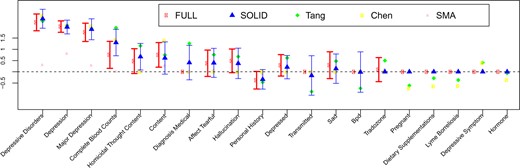
Point estimates and 95% confidence interval of the top 20 non-zero beta coefficient estimates with largest magnitudes obtained by the proposed SOLID method and its competing methods.
Comparisons among the external validation (EXT), apparent validation (APP), and MCV in regards to averaged computing time, averaged difference compared to the external validation (DIFF), empirical standard error (ESE), averaged approximate standard error (ASE), and coverage probability (CP) of area under the curve (AUC) and sensitivity.
| AUC | Sensitivity | |||||||||
|---|---|---|---|---|---|---|---|---|---|---|
| Method | Time | DIFF | ESE | ASE | CP (%) | DIFF | ESE | ASE | CP (%) | |
| EXT | 7.5 | — | 0.00413 | — | — | — | 0.00320 | — | — | |
| APP | 7.6 | 0.00927 | 0.00468 | — | 52.1 | 0.03055 | 0.01779 | — | 62.7 | |
| MCV | 35.0 | 0.00006 | 0.00448 | 0.00422 | 92.3 | |$-$|0.00122 | 0.01536 | 0.01447 | 92.9 | |
The proposed SOLID algorithm was implemented as an R software package solid, which is available at https://github.com/celehs/solid.
4. Data application
The EMR contains rich clinical information on patients including medical history, vital signs, lab test results, and clinical notes. Accurately assigning ICD codes for individual patient visits is highly important on many levels, from ensuring the integrity of the billing process to creating an accurate record of patient medical history. However, the coding process is tedious, subjective, and currently relies largely on manual efforts from professional medical coders. The large volume of medical records makes manual ICD assignment a labor-intensive and costly process, signifying the need for methods to automate the coding process. Narrative features can be extracted from free text such as radiology reports via natural language processing (NLP). To explore the feasibility of automatic code assignment based on narrative text, we aim to develop an ICD classification model for depression based on high dimensional NLP features, and to evaluate its accuracy using EMR data from Partner’s Healthcare Biobank (PHB).
The analysis data consisted of ICD codes and NLP features for 1 000 000 visits, which was a random sample of |$2\,096\,563$| visits from PHB. The remaining |$1\,096\,563$| visits were considered as a validation set for model evaluation. The response |$Y$| was the indicator for having at least one ICD code for depression on each visit and the prevalence was about |$4\%$|. A list of |$1410$| candidate medical concepts were extracted by performing named entity recognition on five articles related to depression from online sources including Wikipedia, MedlinePlus, Medscape, Merck, and Mayo Clinic, following the strategy of Yu and others (2016). We then performed NLP on the EMR narrative notes to count the occurrences of these NLP features in each visit. After quality control and pre-screening, we retained a total of 142 NLP features that appeared in at least 5% of the visits. Because the NLP counts tend to be zero-inflated and highly skewed, we took |$x \mapsto \log(x + 1)$| transformation on all features. It is worth mentioning that for the visit level data, the variables were not independent and identically distributed, since the measurements for each patients were correlated. Therefore, we fitted a penalized generalized linear model with independent working covariance for estimation and the sandwich estimator for variance calculation. We set an effective sample size with the number of patients instead of the number of visits for tuning parameter selection and let |$K = 100$| for SOLID estimation. The full sample estimator can only be calculated with a very large memory capacity (120 GB) available.
For regression coefficients, we compare |$\widehat{\boldsymbol{\beta}}_{\sf \scriptscriptstyle{SOLID},j}$|, |$\widehat{\boldsymbol{\beta}}_{\scriptscriptstyle\Omega_{\sf \scriptscriptstyle +}}$|, |$\widehat{\boldsymbol{\beta}}_{\scriptscriptstyle \sf Chen}$|, |$\widehat{\boldsymbol{\beta}}_{\scriptscriptstyle \sf Tang}$|, and |$\widehat{\boldsymbol{\beta}}_{\scriptscriptstyle \sf SMA}$| with regards to computation time, point estimates, and confidence intervals. The proposed SOLID method takes 31 s, while all the other methods take longer times (34 min, 1532 s, 1476 s, and 116 s for |$\widehat{\boldsymbol{\beta}}_{\scriptscriptstyle\Omega_{\sf \scriptscriptstyle +}}$|, |$\widehat{\boldsymbol{\beta}}_{\scriptscriptstyle \sf Chen}$|, |$\widehat{\boldsymbol{\beta}}_{\scriptscriptstyle \sf Tang}$|, and |$\widehat{\boldsymbol{\beta}}_{\scriptscriptstyle \sf SMA}$|, respectively). Bootstrap was used to calculate the standard errors of |$\widehat{\boldsymbol{\beta}}_{\scriptscriptstyle\Omega_{\sf \scriptscriptstyle +}}$|. We present the point estimates for all methods and the confidence intervals for |$\widehat{\boldsymbol{\beta}}_{\scriptscriptstyle\Omega_{\sf \scriptscriptstyle +}}$| and |$\widehat{\boldsymbol{\beta}}_{\sf \scriptscriptstyle{SOLID},j}$| for the 20 predictors with the largest estimated effect sizes in Figure 1. The results for the remaining predictors are summarized in the Supplementary Materials available at Biostatistics online. As expected, for most predictors among the top 20 with largest effect sizes, the point estimates, and confidence intervals of |$\widehat{\boldsymbol{\beta}}_{\sf \scriptscriptstyle{SOLID},j}$| are very close to those of |$\widehat{\boldsymbol{\beta}}_{\scriptscriptstyle\Omega_{\sf \scriptscriptstyle +}}$|. On the other hand, |$\widehat{\boldsymbol{\beta}}_{\scriptscriptstyle \sf Chen}$|, |$\widehat{\boldsymbol{\beta}}_{\scriptscriptstyle \sf Tang}$|, and |$\widehat{\boldsymbol{\beta}}_{\scriptscriptstyle \sf SMA}$| are different with regards to point estimates compared with |$\widehat{\boldsymbol{\beta}}_{\scriptscriptstyle\Omega_{\sf \scriptscriptstyle +}}$|.
We conduct model evaluation of the SOLID algorithm using MCV. For benchmark, we evaluate the full-sample based adaptive lasso algorithm using external validation. We present the receiver operating characteristic curve in Figure 2. The AUCs of proposed method and full-sample based adaptive lasso are 0.908 (95% CI [0.905, 0.911]) and 0.907 (95% CI [0.906, 0.909]), respectively. At FPR = 0.1, the TPRs of the proposed method and the full-sample based adaptive lasso are 0.799 (95% CI [0.792, 0.807]) and 0.797 (95% CI [0.793, 0.800]), respectively; at FPR = 0.15, the TPRs of proposed method and the full-sample based adaptive lasso are 0.864 (95% CI [0.858, 0.870]) and 0.860 (95% CI [0.857, 0.863]). This observation suggests that the accuracy estimates of the SOLID algorithm obtained by the MCV procedure are very close to those of the full-sample based procedure obtained by external validation.
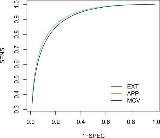
Averaged ROC curves of external validate (EXT), apparent validation (APP), and modified cross validation (MCV) over 1000 simulations.
5. Discussion
In this article, we propose a novel SOLID method for sparse risk prediction and also develop an efficient MCV for model evaluation. The proposed SOLID for fitting adaptive LASSO reduces the computation cost while maintaining the precision of estimation with an extraordinarily large |$n_0$| and a numerically large |$p$|. The use of a screening step and one-step linearization fused DAC makes it feasible to obtain a SOLID estimator that attains equivalent precision to that of the full sample estimator with a many-fold reduction of computation time. The purpose of the screening steps (1.1)–(1.4) is to choose the active set, while that of the post screening steps (2.1) and (2.2) is to get the refined estimation results. Specifically, although the active set estimate |$\widehat{{\cal A}}$| from the screening step consistently estimates |$\mathcal{A}$| asymptotically, it may not be sufficiently accurate since it is derived based on a “rough” one-step estimator |$\widetilde{\boldsymbol{\beta}}_{\scriptscriptstyle\Omega_{\sf \scriptscriptstyle +}}^{\sf\scriptscriptstyle lin,1}$|, which has a convergence rate of |$\|\widetilde{\boldsymbol{\beta}}_{\scriptscriptstyle\Omega_{\sf \scriptscriptstyle +}}^{\sf\scriptscriptstyle lin,1}-\boldsymbol{\beta}_0\|_2 = O_p(p/n_{\Omega_1})$|, slower than that of |$\widetilde{\boldsymbol{\beta}}_{\scriptscriptstyle\Omega_{\sf \scriptscriptstyle +}}$| when |$n_{\Omega_1}$| is not very large. However, this step is critical in improving the computational speed of SOLID since step (2.1) can be performed much faster when constraining to the estimated active set |$\widehat{{\cal A}}$|. The time costs needed to implement each step of the SOLID algorithm in comparison with the direct DAC without screening are summarized in the Supplementary Materials available at Biostatistics online. To examine the performance of variable selection in the screening procedure, we summarize the size of the estimated active set, sensitivity (the proportion of actual active features that are correctly identified by the algorithm), specificity (the proportion of nonactive features that are not identified by the algorithm) in the Supplementary Materials available at Biostatistics online.
The estimator substantially outperforms existing DAC procedures with respect to both computational time and estimation accuracy. One major difference between the SOLID algorithm and the existing DAC algorithm is that we combine data from all subsets to calculate the information matrix |${\widehat A}_{\sf \scriptscriptstyle{DAC}}$|, while other methods only perform estimations on individual subsets which essentially rely on an information matrix estimated from the subsets. When |$p$| is large, the approximation error of the information matrix estimated from each subset is substantially larger compared to the approximation error of the aggregated counterpart. We find that the improved precision of |${\widehat A}_{\sf \scriptscriptstyle{DAC}}$| contributes significantly to the performance of the SOLID estimator, especially for settings with weaker signals. For example, Chen and Xie (2014) essentially uses individual sets to calculate the information matrix and the score and then combine estimates across |$K$| parts via majority voting. Compared to their estimator, the SOLID estimator has a much smaller MSE when signals are weaker (simulation settings 2 and 3) and |$p$| is large.
For our numerical studies, we required |$K$| to be of order |$o(n_0^{1/2})$| and fixed it to be |$100$| with |$p=50$| and |$500$| and |$50$| when |$p=1000$|. Here, we give a few practical guidelines to the choice of |$K$|. The partition size |$K$| should be chosen to ensure that |$n$| is reasonably larger than |$p$|, say |$n >5p$|, as well as large enough to benefit from distributed execution. In our numerical studies, we did not use parallel computing for calculating the statistics on the individual subsets due to computing resource constraints. However, we highly recommend using multicore and multi-node parallel computing to maximize the efficiency of the SOLID algorithm. In step (1.1) of the screening step, we used data in |$\Omega_1$| to obtain an initial estimator. When the event rate is low and |$p$| is large, one may combine several subsets to calculate the initial estimator to improve stability. When |$p$| is also very large, it is possible that the proposed SOLID algorithm is still subject to computational limitations with |$n > p$|. For such settings, additional refinement such as those adopted in sure independence screening (Fan and Lv, 2008). Future research is needed for additional model assumptions that may be needed to improve the screening step.
Supplementary material
Supplementary material is available at http://biostatistics.oxfordjournals.org.
