


Summary
A great deal of neuroimaging research focuses on voxel-wise analysis or segmentation of damaged tissue, yet many diseases are characterized by diffuse or non-regional neuropathology. In simple cases, these processes can be quantified using summary statistics of voxel intensities. However, the manifestation of a disease process in imaging data is often unknown, or appears as a complex and nonlinear relationship between the voxel intensities on various modalities. When the relevant pattern is unknown, summary statistics are often unable to capture differences between disease groups, and their use may encourage post hoc searches for the optimal summary measure. In this study, we introduce the multi-modal density testing (MMDT) framework for the naive discovery of group differences in voxel intensity profiles. MMDT operationalizes multi-modal magnetic resonance imaging (MRI) data as multivariate subject-level densities of voxel intensities and utilizes kernel density estimation to develop a local two-sample test for individual points within the density space. Through simulations, we show that this method controls type I error and recovers relevant differences when applied to a specified point. Additionally, we demonstrate the ability to maintain power while controlling the family-wise error rate and false discovery rate when applying the test over a grid of points within the density space. Finally, we apply this method to a study of subjects with either multiple sclerosis (MS) or conditions that tend to mimic MS on MRI, and find significant differences between the two groups in their voxel intensity profiles within the thalamus.
1. Introduction
Clinical interpretation of brain magnetic resonance imaging (MRI) scans has long been a vital tool for the detection and treatment of neurological diseases (Edelman and Warach, 1993). In the past few decades, quantification and statistical analysis of data from MRI scans have provided additional value for not only diagnosing and monitoring such diseases, but also for understanding brain development (Gu and others, 2015), human behavior (Phelps and LeDoux, 2005), and psychiatric disorders (Xia and others, 2018). As MRI technology has improved, the data derived from MRI scans have increased in scale and complexity, with different scanning modalities each producing intensity values at hundreds of thousands of voxels (3D pixels) within the brain. To accommodate the dimensionality of these data, numerous statistical techniques have been developed to allow researchers to locate and carry out inference on potential disease signatures in these scans (e.g., Winkler and others, 2014; Vandekar and others, 2018).
Research using neuroimaging data has largely followed two main frameworks: identifying effects that occur in specific regions of the brain by conducting voxel-wise or region-of-interest (ROI) analysis, and identifying and segmenting tissue types that can be located spatially and studied as cohesive structural units. However, the application of these two frameworks makes the implicit assumption that either, (i) the relevant intensity signature will occur (or not occur) in the same voxels for every subject (e.g., voxels within the amygdala showing increased blood flow during emotion tasks), or (ii) the relevant intensity signature will be localized in space and will show enough contrast with its surroundings to allow for segmentation and subsequent analysis (e.g., tumors and lesions). We now know, however, that some diseases are characterized by diffuse processes that can be invisible to these techniques. For example, recent research has found subtle differences between multiple sclerosis (MS) subjects and healthy controls within the normal-appearing white matter (NAWM) of the brain, taking the form of slight mean and variance shifts in the intensity of the NAWM voxels (Whittall and others, 2002; Lund and others, 2013).
To study these processes, prior work has often relied on univariate or bivariate summary statistics (e.g., mean, standard deviation, correlation) or histogram analysis to characterize the intensities present in this tissue. However, when processes are complex or multivariate, these techniques may fail to capture the true nature of the relevant intensity signatures, and post hoc efforts to find a summary statistic sensitive to these effects can introduce substantial bias through implicit multiple comparisons. When potentially diffuse processes are of interest, quantifying the joint relationships of voxel intensities across modalities can help fill this methodological gap. Some work has begun conceptualizing neuroimaging data in this way, such as intermodal coupling (Vandekar and others, 2016) and spatial correspondence testing (Alexander-Bloch and others, 2018). However, some of these methods rely on summaries or voxel-wise analyses that have the potential to present only a limited view of each subject’s multivariate intensity space, and others do not easily scale to higher dimensional intensity spaces.
Here, we propose treating subjects’ high-dimensional, multi-modal data as being drawn from subject-level multivariate densities. This framework draws ideas from various related works. Specifically, omnibus tests for detecting overall group differences in multivariate densities can be performed using a distance-based testing framework (Reiss and others, 2010), yet limited information is obtained from such an omnibus test. When more specific quantification of differences is desired, histogram analysis has typically been used in neuroimaging to quantify the shape of voxel intensity densities (e.g., Giulietti and others, 2018; Mascalchi and others, 2018). However, such histogram analysis methods focus on univariate densities from a single imaging modality and rely on summary values like peak locations and skewness. When joint densities across multiple modalities are of interest, researchers would likely learn more from local tests performed at specified points within the density space. Prior research has proposed a procedure for local testing across two group-level multivariate densities (Duong, 2013), utilizing kernel density estimators (KDEs), and leveraging their known asymptotic behavior to develop the test. However, in the context of neuroimaging, the local comparison of two group-level densities represents a special case where two subjects are being compared directly and the only source of uncertainty is the variance arising from the KDE.
This study seeks to extend these existing methods to the setting in which densities arise at the subject level, and differences in the local means of group-specific densities are of interest. A similar context was explored in a previous applied study, in which differences in subject-level bivariate densities were detected using cluster-extent analysis (Zhang and others, 2010). In the current study, we build on that work by developing the multi-modal density test (MMDT), a formal test for local group differences in subject-level multivariate densities, and describing its asymptotic and small-sample properties. In Section 2, we introduce the test statistic and discuss its asymptotic properties. In Section 3.1, we conduct simulation studies to investigate performance of the local test as the number of subjects per group and the number of datapoints per subject vary. In Section 3.2, we simulate the performance of four potential multiple comparison adjustments when conducting the MMDT over a grid of points within the density space. Finally, in Section 4, we apply the MMDT to MRI data from subjects with MS and subjects with other conditions that have similar MRI presentations, in order to investigate possible differences in thalamic intensity profiles.
2. Proposed method
We seek to investigate local differences in |$d$|-dimensional multivariate densities |$f_i$|, |$i=1,\dots ,n$|, between two groups. As this work focuses on the application to neuroimaging data, the |$d$|-dimensional multivariate space can be thought to refer to the space of voxel intensities across |$d$| different imaging modalities. Let |$s_i \in \{0,1\}$| be a binary group indicator for subject |$i$|. Further, define group |$\mathcal{A} = \{ i: s_i = 0 \}$| and group |$\mathcal{B} = \{ i: s_i = 1 \}$|. We assume each subject has a subject-specific density |$f_i$|, so that |$f_i(\mathbf{x})$| represents the density of the ith subject evaluated at a given point, |$\mathbf{x} \in \mathbb{R}^{d}$|.
Given the presence of between-subject variability in the relative composition of different voxel phenotypes, we assume the local subject-level densities, |$f_i(\mathbf{x})$|, to be themselves characterized by a group-specific distribution,
Assuming that the densities |$f_i$| are bounded and continuous, it follows that for |$g \in \{\mathcal{A},\mathcal{B}\}$| and |$\mathbf{x} \in \mathbb{R}^{d}$|, |$F^*_g(\mathbf{x})$| has mean |$\mu_g(\mathbf{x})$| such that |$\mu_g(\mathbf{x})<\infty$|, and variance |$\sigma^2_g(\mathbf{x})$| such that |$0<\sigma^2_g(\mathbf{x})<\infty$|. At the point |$\mathbf{x}$|, we are interested in testing the local hypothesis |$H_0(\mathbf{x}): \mu_\mathcal{A}(\mathbf{x}) = \mu_\mathcal{B}(\mathbf{x})$|. If we could observe the densities, |$f_i(\mathbf{x})$|, directly and without noise, we could estimate |$\mu_\mathcal{A}(\mathbf{x})$| and |$\mu_\mathcal{B}(\mathbf{x})$| by
where |$n_g$| is the sample size of group |$g \in \{\mathcal{A}, \mathcal{B}\}$|,
However, in practice we do not directly observe subjects’ densities |$f_i$|. Instead, for subject |$i$|, we observe a sample of |$v_i$| voxels, |$\mathbf{X}_i$|, from the true multivariate density |$f_i$|, where
Here, |$X^{(1)}$| represents voxel 1, which is characterized by |$d$| different intensity values derived from |$d$| different imaging modalities. Using the observed voxels, we can obtain the kernel density estimate of |$f_i$| as follows:
where K is the kernel function with |$K_{\mathbf{H}_i}(\mathbf{x})=|\mathbf{H}_i|^{-1/2}K(\mathbf{H}_i^{-1/2}\mathbf{x})$| and |$\mathbf{H}_i$| is a bandwidth matrix for subject |$i$|. For an individual kernel density estimate, we assume that:
(1) the true density |$f_i(\mathbf{x})$| is bounded and continuous,
(2) the bandwidth matrices, |$\mathbf{H}_i=\mathbf{H}_i(v_i)$|, represent a sequence of positive definite matrices in which the elements of |$\mathbf{H}_i \rightarrow 0$| and |$v_i^{-1} |\mathbf{H}_i|^{-1/2} \rightarrow 0$| as |$v_i \rightarrow \infty$|,
(3) and the kernel K is a symmetric, square integrable probability density function, such that |$\int_{\mathbb{R}^d} \mathbf{xx}^T K(\mathbf{x}){\rm d}\mathbf{x}=m(K)\mathbf{I}_d$| for some real number |$m(K)$|, and |$R(K)=\int_{\mathbb{R}^d}K(\mathbf{x})^2{\rm d}\mathbf{x}<\infty$|.
Under these conditions, prior work (Parzen, 1962; Wand, 1992) has shown that |$\hat{f_i}(\mathbf{x; H_i}) \overset{d}{\rightarrow} N(f_i(\mathbf{x}),\omega_i)$| as |$v_i \rightarrow \infty$|, where |$\omega_i=v_i|\mathbf{H_i}|^{-1/2}R(K)f_i(\mathbf{x})$|. While these classical proofs of asymptotic normality relied on an assumption of independence, recent work has extended those results to show that asymptotic normality holds for sequentially (Dedecker and Merlevede, 2002) and spatially (El Machkouri, 2011) dependent data. Thus, as |$v_i \rightarrow \infty$|, we can consistently estimate |$\mu_g(\mathbf{x})$| by
Due to the uncertainty imposed by the KDE, additional variance, |$\omega_i$|, is imposed on the subject-level densities. Yet because |$\omega_i \rightarrow 0$| as |$v_i \rightarrow \infty$|, the target variance in each group, |$\sigma^2_g(\mathbf{x})$|, can still be consistently estimated by the sample variance,
Finally, under the local null hypothesis |$H_0(\mathbf{x}): \mu_{\mathcal{A}}(\mathbf{x}) = \mu_{\mathcal{B}}(\mathbf{x})$|, we can construct a test statistic given by the following,
Allowing for unequal variances, this test takes the form of Welch’s two-sample t-test. The statistic, |$t(\mathbf{x})$|, then follows a |$t$| distribution with |$\delta$| degrees of freedom, and converges in distribution to |$N(0,1)$| as |$n_\mathcal{A}, n_\mathcal{B} \rightarrow \infty$|. Here,
Notably, the performance of this test depends on large samples of within-subject observations, as well as either a large number of subjects or relatively symmetric group-level data. While the limit |$n \rightarrow \infty$| in this context bears the familiar interpretation of the sample size going to infinity, the limit |$v_i \rightarrow \infty$|, which indicates the number of voxels per subject going to infinity, is less standard. In practice, this assumption can be thought to represent improvements in MRI technology, which have led to voxels representing smaller and smaller spatial regions over the past few decades. To understand the importance of this limit for the method’s validity, in the following section we describe and conduct simulation studies across finite voxel and sample sizes.
3. Simulation study
To determine the finite-voxel and finite-sample performance of the MMDT procedure, we conducted two simulation studies. The first examined the performance of the local test conducted at a specific point in the multivariate density space, |$\mathbf{x}$|, to assess the validity of the test statistic’s null distribution and determine its power. The second examined the performance of the method when applied over a grid of points across the density space, to characterize the full exploratory use case and illustrate potential methods for accounting for multiple comparisons in this setting. Both studies were comprised of several scenarios to examine how the findings were affected by features of the data generating distribution and user choices required by the method.
For both simulation studies, observations for each subject were drawn from a mixture of a shifted and scaled bivariate beta distribution and a bivariate normal distribution. This set-up thus reflects a scenario in which voxels each have two associated intensity values (|$d=2$| modalities). Group differences were implemented in the correlation structure of the bivariate beta distribution, while the form of the bivariate normal distribution was consistent across groups (see Figure 1). Inverse transform sampling was used on bivariate normal observations in order to simulate bivariate beta observations with a specific correlation structure.
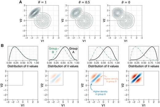
Design of the simulation studies. (A) Illustration of the voxel intensity generating distributions across values of |$\theta$|. (B) Visualization of the expected group differences in densities across simulation scenarios. The first column shows the scenario in which |$\theta$| values are drawn from the same beta distribution for subjects in group A and group B. Second, third, and fourth columns show the scenarios in which |$\theta$| values are drawn from increasingly divergent beta distributions for subjects in Group A and Group B.
We chose this set-up, instead of a single bivariate normal distribution, for two primary reasons: (i) The mixture distribution allowed us to isolate specific regions in which there is a group difference, while also examining the performance of the test in regions where there is no group difference. Specifically, since the scaled bivariate beta distribution has finite support, its use creates a bounded false null region. Had a single bivariate normal distribution been used, any group difference in its covariance structure would create a globally false null. In short, the chosen scenario allows us to consider both a mixed null case and a global null case. (ii) The mixture distribution gives a scenario in which simple univariate and bivariate summary statistics are not well-suited to characterize the group difference. This then demonstrates a case where the proposed method would be able to capture on group differences that are obscured by subject-level means or correlations.
The density takes the following form:
where,
For each subject, a value for |$\theta$|, the parameter that drives the correlation of the bivariate beta observations, |$r$|, was drawn from a beta distribution with group-specific values for parameters |$\alpha$| and |$\beta$|. When |$\alpha_A\neq\alpha_B$| and/or |$\beta_A\neq\beta_B$|, this parameter induced differences in the groups’ mean bivariate densities and subject-specific variation within group.
3.1. Testing at a single point
For the first simulation, four data generating scenarios were included. The first, designed to examine type I error, specified |$\alpha_A=\alpha_B=2$| and |$\beta_A=\beta_B=5$|, meaning that there was no group difference in the correlation structure of the bivariate beta observations (i.e., a global null case). The remaining three simulation scenarios examined the test’s power (in the false null regions) and type I error (in the true null regions) for varying degrees of discrepancy between group densities. In the three scenarios, |$\alpha_A=\beta_B=5$|, and |$\alpha_B$| and |$\beta_A$| were set at 4, 3, and 2, respectively.
Each simulation scenario was repeated with a variety of between-subject sample sizes, |$n$|, and within-subject observations, |$v$|. The effect of the number of subjects per group on type I error and power was tested using |$n_A=n_B=20, 30, 50,$| and |$80$|. The effect of the number of observations per subject was tested using |$v_i=500, 1000, 2500, 5000,$| and |$10\,000$| for all |$i$|. Each scenario (i.e., combination of |$n$| and |$v=v_i$|) was run 1000 times. For the presented simulations, the ks package in the R Statistical Environment was used to compute subject-level KDEs (Duong, 2007; R Core Team, 2018). KDEs were calculated using normal kernels, and bandwidth matrices were empirically estimated using the plug-in estimators proposed by Duong and Hazelton (2003). Results of the simulation studies are presented for four exemplary points within the bivariate density space: |$\left [x_1=-2; x_2=2 \right ]$|, |$\left [x_1=-1.5; x_2=1.5 \right ]$|, |$\left [x_1=0; x_2=-1 \right ]$|, and |$\left [x_1=-2.5; x_2=-0.1 \right ]$|. These points were selected a priori to represent different density levels (in both type I error and power analyses) and different degrees of group differences (in power analyses).
For the global null case, in which |$\alpha_A=\alpha_B=2$| and |$\beta_A=\beta_B=5$|, type I error was controlled at |$\alpha=0.05$| for all four points, across all combinations of |$n$| and |$v$|. This suggests that the distribution of the test statistic is valid in settings with small-to-medium sample sizes and subject-level observations (Figure 2, column 1). Importantly, this was true when the correlation-generating parameter, |$\theta$|, was drawn from a skewed distribution.
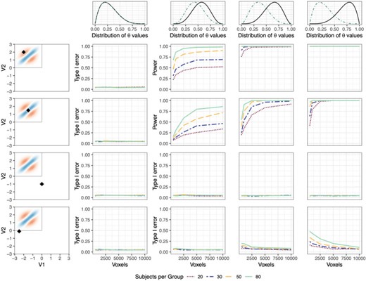
Type I error and power of MMDT applied to a single point. Columns represent the four simulation scenarios, in which |$\theta$| values are either drawn from the same beta distribution for subjects from both groups (column 1) or increasingly divergent beta distributions (columns 2–4). Rows show the rate at which the local null hypothesis is rejected at four exemplary points in the density space. Rows 1 and 2 show points at which there is a true group difference in the generating distribution. Rows 3 and 4 show points at which there is no true group difference in the generating distribution. Each plot shows the rejection rate as a factor of the number of voxels per subject and the number of subjects per group.
Simulation results for the three scenarios in which there were group differences reveal the interplay between sample size and subject-level observations in obtaining adequate power. Figure 2 (row 1, columns 2–4) represents the power of the local test for a point at which one group tends to have a low density of voxels, while the other has a moderate density. Here, sample size appears to play a greater role than subject-level observations in obtaining power to detect the difference. Row 2 (columns 2–4) represents a point at which there is a meaningful group difference, but densities tend to be relatively high in both groups and the region of difference is somewhat narrow. Here, the number of subject-level observations appears to play a slightly larger role in obtaining adequate power, potentially suggesting that accurate kernel density estimation is important for detecting group differences in regions where the difference is more localized. Row 3 (columns 2–4) represents a point at which there is no true difference in the data generating distribution between groups. Unlike the regions illustrated in row 1 and row 2, the detection of significant differences here represents type I error, not power. This row demonstrates that regardless of sample size or number of within-subject observations, the type I error rate is controlled at |$0.05$|.
Finally, row 4 (columns 2–4) represents another point at which there is no true difference between groups. However, unlike the point shown in row 3, this point is adjacent to the false null region. The figure shows that in this case, a low number of subject-level observations (voxels) results in type I error above the nominal rate of |$\alpha=0.05$|, while the type I error rate tends towards |$0.05$| as the number of subject-level observations increases. The inflated type I error rate in this region is an artifact of the smoothing that results from the KDE in the presence of low numbers of observations. Specifically, in the presence of low numbers of voxels the plug-in bandwidth estimators utilize observations from a wider range of locations to estimate local densities, which has the potential to smooth differences from the false null region (the gray box in the upper left hand corner) into the true null region. This issue suggests that the strict local interpretation of the test may be limited in situations in which few voxels are analyzed per subject, though importantly, this effect is only seen very close to the border of the false null region.
3.2. Testing over a grid
In most cases, researchers will not have a limited set of points at which they wish to test for group differences. Instead, a more common use case will likely be to conduct an exploratory test for differences over a dense grid of points throughout the multivariate space. To conduct this type of analysis, the issue of multiple comparisons must be addressed (e.g., conducting the MMDT on a 151 |$\times$| 151 grid yields 22 801 individual test statistics). Countless methods have been proposed to adjust for multiple comparisons in high-dimensional cases. Here, we will compare the performance of four methods—two for controlling the family-wise error rate (FWER) and two for controlling the false discovery rate (FDR)—and discuss the benefits and limitations of each.
For controlling FWER, we apply the max-t procedure (Westfall and Young, 1993) and threshold-free cluster enhancement (TFCE) procedure (Smith and Nichols, 2009). The max-t procedure calculates pointwise significance by comparing the test statistics in the observed comparison to a distribution of maximum test statistics obtained through permutation of group labels. This test is well-suited to account for dependence between test statistics and is primarily suited for testing the global null (i.e., all hypotheses are true). Its power and ability to control FWER in the mixed null case (i.e., some hypotheses are false) are less clear. TFCE more explicitly accommodates spatial dependence between test statistics, as would be expected when testing multiple points across the density space. TFCE incorporates spatial dependence by augmenting pointwise test statistics with their membership, or lack thereof, in spatial clusters. Forgoing the pre-specification of a specific cluster-forming threshold, TFCE’s augmentation incorporates information from the full range of possible thresholds. Like max-t, TFCE compares the resulting pointwise scores to the distribution of the maximum scores under permutation of group labels, and is also primarily suited for testing the global null. Its incorporation of spatial extent makes it likely to be more powerful than max-t in this context, but its ability to control FWER under a mixed null depends on the assumption of subset pivotality, which is almost certainly violated due to the smoothness of the kernel density estimates.
For controlling FDR, we apply both the Benjamini–Hochberg (BH) (Benjamini and Hochberg, 1995) and Benjamini–Yekutieli (BY) (Benjamini and Yekutieli, 2001) procedures. BH is the classical method for FDR control, in which p-values are ordered from small to large and significance is determined for ordered test |$i$| by whether or not the p-value, |$p_i\leq\alpha*\frac{i}{m}$|, where |$\alpha$| is a preselected significance level, and |$m$| is the total number of tests (Benjamini and Hochberg, 1995). This method controls the FDR under independence or positive regression dependence of individual p-values. BY is a more conservative adjustment to the BH procedure that allows for arbitrary dependence between p-values (Benjamini and Yekutieli, 2001). Since positive dependence is a reasonable assumption in this context (i.e., differences in one region are positively linked with the presence of differences in another region), we expect BY may be overly conservative. Importantly, FDR is best defined in the mixed case, in which some null hypotheses are false. In the global null case, in which all null hypotheses are true, FDR is equal to FWER.
Simulated comparison of these four adjustment techniques was carried out using the same data generation procedure described previously. Results are presented for the situation when |$n_A=n_B=30$|, with the number of voxels per subject, |$v_i$|, varied over |$500, 1000, 2500, 5000,$| and |$10\,000$|. To assess FWER under a global null, the scenario in which |$\alpha_A=\alpha_B=2$| and |$\beta_A=\beta_B=5$| was used. To assess power, FWER under the mixed null, and FDR under the mixed null, the scenario in which |$\alpha_A=\beta_B=5$| and |$\alpha_B=\beta_A=3$| was used. Each scenario was tested 1000 times, and the corrected p-values for each point were obtained using each of the four procedures described above.
Figure 3 shows the power at two exemplary points (row 1), FWER and FDR in the mixed null case (row 2), and FWER in the global null case (row 3). Row 1 shows increasing power for all multiple comparison procedures as the number of voxels increases. Taking the case of 5000 voxels as an example, power is |$0.82$| with max-t correction, |$0.93$| with TFCE, |$0.98$| with BH, and |$0.88$| with BY at |$[x_1=-2, x_2=2]$| (shown in red), and |$0.24$|, |$0.62$|, |$0.82$|, and |$0.48$|, respectively, at |$[x_1=-1.5, x_2=1.5]$| (shown in blue). Consistent with expectations, TFCE obtains additional power above max-t by incorporating cluster information, and BH achieves higher power than both FWER methods by controlling FDR. BY, due to its conservative nature, obtains power somewhere between the TFCE and max-t procedures.
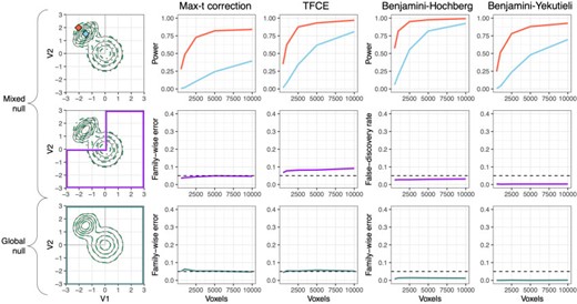
Type I error and power of MMDT applied over a grid. Columns represent the four multiple comparison methods being compared. Row 1 shows the power for two exemplary points at which there is a true group difference in the data generating distribution. Row 2 shows the FWER (columns 1 and 2) and the FDR (columns 3 and 4) in the mixed null case, with the purple box highlighting the region of the density space at which there is no true group difference in the data generating distribution. Row 3 shows the FWER in the global null case, with the green box highlighting the full density space, across which there is no true group difference in the data generating distribution.
Row 2 shows results for the mixed null case, in which hypotheses in the upper square of the density space are false, and hypotheses in the rest of the density space are true. Here, the number of subject-level observations does not seem to impact either FWER or FDR. Across these values, the average FWER is |$0.043$| using max-t and |$0.081$| using TFCE, while the average FDR is |$0.028$| using BH and |$0.003$| using BY. The lack of FWER control under TFCE in the mixed case is partly due to its lack of a clear pointwise interpretation; TFCE only allows for an interpretation along the lines of, “there exists a cluster containing this point for which we reject the null, and we conclude that there is signal for at least one point within that cluster.” Thus, while TFCE does provide increased power over max-t, its lack of strict FWER control in the mixed case and its lack of clear pointwise interpretation make it perhaps less than ideal in this context. As expected, BH controls FDR slightly below the nominal rate, while BY is overly conservative. Row 3 shows the results for the global null case, in which all hypotheses are true. Across subject-level observation counts, the average FWER is |$0.053$| using max-t, |$0.052$| using TFCE, |$0.012$| under BH, and |$<0.001$| for BY, demonstrating that FWER error is controlled for all four methods under a global null.
4. Application: thalamic intensity profiles in MS
MS is an autoimmune inflammatory demyelinating disease of the central nervous system. MS is typically characterized on MRI by lesions in the white matter of the brain (Trip, 2005) and is clinically characterized by cognitive and motor impairment (Chiaravalloti and DeLuca, 2008; Kurtzke, 1983). While neuroimaging research in MS has largely focused on the characterization of lesional and axonal damage in the white matter (Trip, 2005; Barnett and others, 2016), a growing body of work has also shown that loss of gray matter tissue (referred to as “atrophy”) is also common in MS (Minagar and others, 2013). The thalamus, one of several gray matter structures in the brain, appears to be particularly relevant in MS pathology. Studies have found that MS subjects show greater rates of thalamic atrophy than healthy controls (Houtchens and others, 2007), MS subjects have differing spatial patterns of thalamic atrophy compared to healthy controls (Fadda and others, 2019), and specific thalamic markers are related to worse clinical outcomes within MS subjects (Rocca and others, 2010).
Despite the prevalence of literature comparing the thalami of MS subjects to those of healthy controls, less is currently known about whether and how thalamic tissue differs between subjects with MS and those with conditions like migraine or small-vessel ischemia that mimic MS on other MRI measures. Notable recent work in this area has found that thalamic volume tends to be lower in MS subjects than subjects with MS mimics (Solomon and others, 2017). This difference potentially implies higher rates of atrophy within MS, and suggests that that differences may also be present within thalamic tissue prior to atrophy. Here, we extend these findings by attempting to flexibly characterize differences in the thalamic voxel intensity profiles between subjects with MS and those with MS mimics. The existence of such differences could give insight into the underlying processes that facilitate increased atrophy in MS.
4.1. Data description
Thirty-nine subjects were recruited from the University of Vermont neurology clinic as part of a study seeking to improve differential diagnostic accuracy in MS (Solomon and others, 2018). Participants were between the ages of 20 and 67, and 36 were women. Ten had MS and had no additional conditions associated with white matter abnormalities; 10 had MS and at least one other condition associated with white matter abnormalities; 10 had migraine with white matter abnormalities visible on MRI; and 9 were previously incorrectly diagnosed with MS and had white matter abnormalities on MRI. All subjects in the sample presented with at least one white matter lesion on MRI. Details of the image acquisition have been previously published (Solomon and others, 2018) and are briefly summarized below.
Whole-brain 3D T|$_1$|-weighted (T1) and fluid-attenuated inversion recovery (FLAIR) volumes (see Figure 4(A)) were acquired on a 3 Tesla (3 T) MRI scanner (Philips dStream, 32-channel head coil). T1 and FLAIR represent two common types of MR image that can be obtained by varying the radio frequency pulses of the scanner, producing differences in contrast and highlighting different qualities of the tissue. Both sequences were obtained in a single scanning session for each subject and were acquired with 1 mm isotropic voxel sizes. All images were preprocessed prior to analysis. Inhomogeneity was corrected using the N4 bias correction method (Tustison and others, 2010), subjects’ FLAIR volumes were rigidly co-registered to their T1 images using a Lanczos windowed sinc interpolator, and extracerebral voxels were removed using multi-atlas skull stripping (Doshi and others, 2013). Finally, the thalamus was segmented from each subject’s T1 volume using joint label fusion (Wang and others, 2013).

Application of the MMDT procedure for testing thalamic intensity profiles. (A) Visualization of four example subjects and their T1 and FLAIR volumes, with thalami highlighted in red. (B) Scatterplots and kernel density estimates for the subjects’ bivariate voxel intensity densities. (C) Results of the MMDT for detecting density differences between MS and non-MS (nMS) subjects. Top row shows the test-statistic map across the bivariate density, bottom row shows significant regions following Benjamini–Hochberg correction. (D) Example of MMDT test statistics being mapped back to subjects’ brain spaces for exploratory visualization.
4.2. Statistical analysis
For each subject, voxels’ T1 and FLAIR intensity values were evaluated within the thalamus (Figures 4(A) and (B)). Intensities were Z-score normalized to remove marginal mean and variance differences across subjects and isolate differences in the joint intensity distributions. Approximately 28 000 thalamic voxels were included per subject (|$M=27748$|, sd = 3283). Subjects’ KDEs were created using a normal kernel with plug-in bandwidth estimators (Duong and Hazelton, 2003), yielding multivariate densities with |$d=2$| modalities (T1 and FLAIR; see Figure 4(B)). MMDT was carried out over a |$151\times151$| grid within the density space from |$[-3,-3]$| to |$[3,3]$|. This range corresponds to the region of the density that includes voxels with normalized T1 and FLAIR values between |$-3$| and |$3$|, capturing roughly 98% of all voxels (|$M=0.98$|, sd = 0.006). Significance was established using the Benjamini–Hochberg procedure (Benjamini and Hochberg, 1995).
4.3. Results
Testing revealed significant differences in the thalamic voxel intensity profiles between MS and nMS subjects. Specifically, MS subjects tended to have higher densities along the |${\rm FLAIR}=-T1$| line, and lower densities in regions of relatively high or low intensity on both T1 and FLAIR (Figure 4(C)). This result indicates that voxels’ T1 and FLAIR intensities within the thalami of MS subjects tended to show more coherence than those of non-MS subjects. A test for group differences in the subject-level correlations between T1 and FLAIR intensities showed some evidence that T1/FLAIR correlations may be slightly higher in MS subjects, though the findings were inconclusive (|$t_{37}=1.48$|, |$p=0.15$|) prior to removal of an outlier in the MS group (|$t_{36}=2.42$|, |$p=0.02$|). Though the MMDT findings presented here may reflect a straightforward difference in within-subject correlations, the lack of prior knowledge regarding which summary statistic(s) may be relevant in this case makes the flexibility of the MMDT valuable for detecting and locating such differences. If differences in a specific summary measure were of interest, the non-parametric nature of MMDT would yield reduced power compared to a direct test of that measure. Thus, this technique is best suited for the detection of unknown or complex group differences.
Exploratory visualization of voxels’ test statistics within subjects’ brain spaces was conducted to determine the potential for common spatial patterning of MS-specific intensity profiles (Figure 4(D)). This process was carried out by assigning voxels the statistic associated with the region of the multivariate density space in which their multi-modal intensities were located. Crucially, these statistics themselves cannot be interpreted in the spatial domain. Instead, the apparent regional partitioning of the test statistics suggests the potential for future work that investigates the relevance of multi-modal voxel intensity profiles within different thalamic subregions.
5. Discussion
In this article, we introduced the MMDT, a method for detecting local group differences in subject-level multivariate densities. The method works by taking multivariate high-dimensional data at the subject level, estimating subject-specific densities (using kernel density estimation), and testing for mean differences in pointwise density values across a binary group variable. In the context of MRI research, MMDT allows researchers to investigate differences in multi-modal voxel intensity profiles, without the assumption that signatures of interest will occur in the same voxels across subjects (as made by mass univariate hypothesis testing). It also allows for the naive detection of group-specific multivariate patterns, reducing the need to perform dimension reduction or select an optimal summary statistic in contexts in which the pattern of interest is not clear.
While the asymptotic properties of the local test as the number of subjects and the number of voxels per subject tend to infinity are straightforward, the behavior of the test with finite samples and relatively few voxels was previously unknown. Thus, we performed simulation studies to investigate the finite-sample properties. The simulations showed that type I error is generally controlled when testing at a single point within the density space. However, with very small numbers of subject-level observations overly smooth kernel density estimates can result in inflated type I error rates along the boundary of false null regions. The simulations also provide insight into the differential effects of voxel number and pointwise density on the power of the test at a given location.
Because of the potential value of this method as an exploratory procedure for detecting previously unknown disease signatures, it is important to be able to simultaneously perform multiple tests over a grid of points within the multivariate density space. In this context, correcting for multiple comparisons is vital. Thus, we conducted a simulation study to compare the performance of max-t correction (Westfall and Young, 1993) and TFCE (Smith and Nichols, 2009) for FWER control, as well as BH (Benjamini and Hochberg, 1995) and BY (Benjamini and Yekutieli, 2001) for FDR control. We found that all four methods controlled FWER under a global null, for which there were no false null hypotheses at any point in the density space, while TFCE failed to control FWER under a mixed null (though, importantly, TFCE does not claim to provide strict pointwise interpretations). BH yielded the highest power of the four methods, followed by TFCE. Due to its control of FDR and high power, we recommend BH among the four tested multiple comparison methods.
We then applied the MMDT to a dataset of structural MRI volumes in MS subjects and subjects with other conditions associated with MRI abnormalities, and sought to detect differences between groups in their voxel intensity profiles within the thalamus. We found significant differences within several regions of the bivariate T1-FLAIR density space, with MS subjects having higher densities in regions that followed more tightly along the |${\rm FLAIR}=-T1$| line, and non-MS subjects having higher densities in the upper-right and lower-left quadrants of the joint space. The results generally suggested that subjects with MS have stronger coherence between T1 and FLAIR intensities among voxels in the thalamus, possibly indicating that a greater proportion of thalamic intensity variability in MS subjects is due to underlying tissue biology versus random scanner noise. Future work could directly incorporate histology data to better understand the underpinnings of these differences in the joint T1-FLAIR space.
Several extensions of this method would be valuable areas to explore in future work. First, neuroimaging data are often characterized by measurement error arising from voxel resolution, motion, and even subjects’ hydration level. Future work could investigate how various types of measurement error affect the performance of this method. Additionally, in cases where spatial localization is of interest, test statistics and p-values from the density space can be visualized in subjects’ scans by matching specific voxels’ multi-modal intensity values with the relevant region of the density space. While these values themselves cannot be interpreted spatially, shared localization of group-specific voxel intensity profiles could be useful for hypothesis generation and motivation of further research.
The analysis of neuroimaging data has revealed countless insights into disease processes in the brain, yet common techniques like voxel-wise significance testing, ROI-based analysis, and network analysis are limited by the assumption that relevant processes will occur in the same locations across subjects. Here, we posited that the operationalization of multi-modal neuroimaging data as subject-level multivariate densities has the potential to reveal diffuse or non-localized imaging signatures, and proposed a method for detecting group differences locally within the density space. We found that this method controls type I error when applied at a single point, controls the FWER when applied over a grid, and maintains power for increasing grid sizes. The MMDT represents an important new tool for the exploratory analysis of neuroimaging data and other high-dimensional subject-level data sources.
Code and data availability
An R package for implementing MMDT is available on GitHub (www.github.com/jdwor/mmdt), and R code for replicating the simulation and application results in this article can be found at www.github.com/jdwor/mmdt_paper.
Acknowledgments
The authors would like to thank the members of the PennSIVE Center and the PICSL group for their feedback on this work, as well as the associate editor and the two anonymous reviewers for their thoughtful and thorough comments on an earlier version of this manuscript.
Conflict of Interest: None declared.
Funding
The project described is supported in part by the NIH grants R01 MH112847 from the National Institute of Mental Health (NIMH) and R01 NS060910 from the National Institute of Neurological Disorders and Stroke (NINDS). The content is solely the responsibility of the authors and does not necessarily represent the official views of the funding agencies. Dr. Solomon has received consulting fees from EMB Serono and Biogen, and research support from Biogen. Dr. Bakshi has received consulting fees from Bayer, Biogen, Celgene, EMD Serono, Genentech, Guerbet, Sanofi-Genzyme, and Shire, and research support from EMD Serono and Sanofi-Genzyme. Dr. Raznahan was supported by the intramural program of the National Institutes of Health (Clinical trial reg. no. NCT00001246, clinicaltrials.gov; NIH Annual Report Number, ZIA MH002949-03).
References
R Core Team. (
