


Summary
In kin-cohort studies, clinicians want to provide their patients with the most current cumulative risk of death arising from a rare deleterious mutation. Estimating the cumulative risk is difficult when the genetic mutation status is unknown and only estimated probabilities of a patient having the mutation are available. We estimate the cumulative risk for this scenario using a novel nonparametric estimator that incorporates covariate information and dynamic landmark prediction. Our estimator has improved prediction accuracy over existing estimators that ignore covariate information. It is built within a dynamic landmark prediction framework whereby we can obtain personalized dynamic predictions over time. Compared to current standards, a simple transformation of our estimator provides more efficient estimates of marginal distribution functions in settings where patient-specific predictions are not the main goal. We show our estimator is unbiased and has more predictive accuracy compared to methods that ignore covariate information and landmarking. Applying our method to a Huntington disease study of mortality, we develop dynamic survival prediction curves incorporating gender and familial genetic information.
1. Introduction
Prediction models are imperative for deciding treatments, communicating prognosis to patients, and designing clinical trials to assess disease-modifying therapies. A challenge to developing prediction models is when the models are based on so-called mixture data, whereby data are collected from multiple populations of interest, but we do not know from which population each observation came. Instead, we only know the probability an observation belongs to each population.
Such mixture data are commonly observed in kin-cohort studies (Wacholder and others, 1998) of mortality in Huntington disease (HD). HD is a rare, genetic disorder caused by a genetic mutation: at least 36 repeats of the trinucleotide cytosine–adenine–guanine (CAG) in the huntingtin gene (Rubinsztein and others, 1996). In kin-cohort studies of HD, genotype information is first obtained from (usually) diseased individuals known as probands. To increase the sample of individuals with the genetic mutation, disease history and mortality information are collected on the probands’ relatives using systematic interviews (Marder and others, 2003). Because of resource constraints, the relatives are not genotyped so we do not know if the relative is truly a carrier or non-carrier of the genetic mutation. But we may compute the probability a relative is a carrier or non-carrier because the mutation is genetically inheritable (Khoury and others, 1993) (see Section S.1. of the Supplementary material available at Biostatistics online for details). Data from the relatives are therefore an example of mixture data: the populations of interest are carriers and non-carriers of the genetic mutation, and each relative’s identity of being a carrier or non-carrier is unknown. Instead, we only know the probability of each relative being a carrier or non-carrier.
Early prediction models for mixture data involved parametric (Wu and others, 2002) and semiparametric (Zeng and Lin, 2007) assumptions of the populations from which data were collected. These models were susceptible to bias when the proposed (semi)parametric models were misspecified.
While nonparametric estimators helped bypass this misspecification, nonparametric maximum likelihood estimators (Wacholder and others, 1998; Chatterjee and Wacholder, 2001; Fine and others, 2004) for mixture data have been shown to be inefficient or not consistent (Wang and others, 2012). Wang and others (2012) and Ma and Wang (2014a) remedied these limitations by developing a class of nonparametric estimators that were consistent and efficient using Hilbert spaces and semiparametric projection (Tsiatis, 2006).
Unfortunately, these nonparametric estimators ignored any auxiliary covariate information that could improve prediction accuracy. Approaches to ameliorate this issue have been proposed but to a limited extent. Ma and Wang (2014b) introduced auxiliary information to a mixture data model where the distribution for each population was modeled semiparametrically. The distributional form, however, was chosen to represent HD after modeling the disease onset process for individuals with the gene mutation (Langbehn and others, 2010). This distributional form is not guaranteed to also represent the survival process for HD. We would need to evaluate the mortality process to accurately choose the distributional form. Wang and others (2017) proposed transformation models to incorporate auxiliary information for each population of the mixture data. The transformations may be completely unspecified, but one must accurately pre-specify the distributions for each mixture population to maximize prediction accuracy. Doing so is difficult without sufficient scientific knowledge. See Garcia and others (2016) for more comparison of all aforementioned methods.
In addition to incorporating auxiliary covariate information to improve prediction accuracy, it is also possible to improve prediction accuracy for individual patients by dynamically updating predictions over time. Dynamic landmark prediction (van Houwelingen and Putter, 2011; Parast and others, 2014) is one framework to achieve this goal whereby predictions for individuals are updated over time, conditioning on the event (e.g., death) not having yet occurred up to a landmark time (i.e., a reference point that takes into account all of the predictor information at that moment). Dynamic landmark prediction is adaptive and more accurate than traditional prediction models which often ignore new information available after baseline, and has not yet been applied to a mixture data setting.
We develop a nonparametric prediction model for mixture data that flexibly incorporates auxiliary covariate information and dynamic landmark prediction. Our contributions are 3-fold. First, we use a fully nonparametric approach to relate censored outcomes from mixture data to auxiliary covariate information. The approach is applicable to any time-to-event outcome and does not require pre-specifying distributional assumptions for the mixture populations. Second, we incorporate dynamic landmark to obtain personalized dynamic predictions over time that uses all updated covariate information. Third, we show our estimator gives more efficient marginal distribution estimates in settings where patient-specific predictions are not the primary goal.
The remainder of the article is as follows. Section 2 describes our proposed estimator, its asymptotic properties, and measures to evaluate prediction accuracy for mixture data. Empirical results in Section 3 show the improved finite sample performance over existing nonparametric methods both in terms of consistency and predictive accuracy. In Section 4, we apply our method to the kin-cohort mortality study of HD, examining the use of gender and CAG repeat length (of the proband) to estimate mortality in the relatives. We then create personalized dynamic risk trajectories over time for relatives whose genotype information is unknown.
2. Dynamic landmark prediction model for mixture data with covariates
2.1. Notation and model framework
Mixture data involve potentially censored outcomes observed from one of |$p$| populations, but population identifiers are unknown. The observed data are |$(X_i,\Delta_i,{\boldsymbol Q}_i,Z_i,W_i)$|, |$i=1,\ldots,n$|, where |$X_i=\min(T_i,C_i)$| and |$\Delta_i=I(T_i\leq C_i)$| with |$T_i$| denoting a failure time and |$C_i$| denoting a continuous random censoring time. We assume |$T_i$| and |$C_i$| are conditionally independent given covariates |$Z_i$| and |$W_i$|, which denote discrete and continuous covariates, respectively. We assume |$Z_i$| and |$W_i$| are one-dimensional, but we discuss extensions to the multivariate case in Section 5.
The failure times |$T_i$| originate from one of |$p$| populations, but we only observe the probability vector |${\boldsymbol Q}_i=(Q_{i1},\ldots,Q_{ip})^T$|, where |$Q_{ik} $| is the probability |$T_i$| originates from population |$k$|, |$k=1,\ldots,p,$| and |$\sum_{k=1}^p Q_{ik}=1$|. We make the following assumptions about |${\boldsymbol Q}_i$|: (i) |${\boldsymbol Q}_i$| is known or exactly estimable from external data. When |${\boldsymbol Q}$| is measured with error, we could use measurement error techniques (Carroll and others, 2006) to assess and correct the misspecification, but this procedure is beyond the current scope of the paper. (ii) |${\boldsymbol Q}_i$| has a discrete distribution with probability mass function |$p_{{\boldsymbol Q}}$| and finite support |${\boldsymbol u}_1,\ldots,{\boldsymbol u}_m$|; (iii) For each possible stratum |$Z=z$| and each neighborhood around |$W=w$|, |$0 < \epsilon < P({\boldsymbol Q}={\boldsymbol u}_j|z,w) < \epsilon < 1$| for all |$z,w$|. This ensures there is a positive probability that an individual belongs to a mixture proportion group.
For the kin-cohort study of HD mortality (Section 4), there are |$p=2$| populations referring to carriers and non-carriers of the genetic mutation. Data are collected on relatives, and for relative |$i$|, |$T_i$| denotes the age of death, and |${\boldsymbol Q}_i=(Q_{i1}, Q_{i2})^T$| contains the probabilities a relative is a carrier and non-carrier, respectively. In the HD study, |${\boldsymbol Q}_i$| is one of |$m=3$| vector values: |${\boldsymbol u}_1=(0.5,0.5)^T, {\boldsymbol u}_2=(0.97,0.03)^T, {\boldsymbol u}_3=(0.75,0.25)^T$|. In terms of covariates, |$Z_i$| denotes the relative’s gender and |$W_i$| denotes the CAG repeat length of the relative’s proband.
Here, |$L$| denotes the population to which a subject truly belongs and can take values from |$1,...,p$|. We use |$L$| only for definition purposes, but |$L$| is not observed in practice. The term |$F_k(t\mid t_0, z,w)$| is the cumulative distribution function for population |$L=k$| with characteristics |$(Z=z,W=w)$| given that the failure time has not yet occurred up to time |$t_0$|.
The time |$t_0$| represents the landmark time which we will use to provide more informative estimates of risk. When |$t_0=0$|, |${\boldsymbol F}(t\mid t_0,z,w)$| is simply a prediction calculated at baseline. When |$t_0>0$|, |${\boldsymbol F}(t\mid t_0,z,w)$| provides updated predictions of survival. For example, in the HD study, where time is on the age scale, individuals in genetic counseling may be interested in learning their estimated survival probability to age 60 given their current age is 50 (i.e., the landmark time |$t_0=50$|) and their covariate information. At a follow-up visit 5 years later, the patient may now be interested to know the updated prediction of surviving to age 60 given they have now survived to age 55 (i.e., the landmark time |$t_0=55$|). Previous work outside the context of mixture data has shown that using updated knowledge of survival improves prediction accuracy (Parast and others, 2014). When covariates |$Z,W$| may also be updated before or at |$t_0$|, these predictions could incorporate these updated values potentially further improving prediction accuracy. In this case, we would write |$Z(t_0)$| and |$W(t_0)$| to be explicit about the dependence on |$t_0$|. Since our numerical studies do not include updated covariates, we use the simplified notation of |$Z,W$| throughout.
2.2. Modified nonparametric kernel Nelson–Aalen estimator
2.2.1. Structure of the main estimator
To estimate |${\boldsymbol F}(t \mid t_0,z,w)$|, we take advantage of the finite support of |${\boldsymbol Q}$|. The finite support implies that each individual uniquely belongs to one of |$m$| different subgroups based on his or her |${\boldsymbol Q}$| value. We will develop estimators for the |$m$| subgroups defined by individuals whose |${\boldsymbol Q}={\boldsymbol u}_j$|, |$j=1,\ldots,m$|, and relate these estimators to |${\boldsymbol F}(t \mid t_0,z,w)$|.
Without covariates and landmarking, the estimator in (2.1) reduces to the estimator of Ma and Wang (2014a). In their work, |$\widehat{\boldsymbol S}(t\mid t_0, z,w)\}$| is replaced by |$\widehat {\boldsymbol S}(t)$| whose |$j$|th component is the Kaplan–Meier estimator based on data for which |${\boldsymbol Q}={\boldsymbol u}_j$|. Our estimator thus generalizes the work of Ma and Wang (2014a) to include covariates and landmark times.
Forming the estimator in (2.1) requires estimating the survival vector |${\boldsymbol S}(t \mid t_0, z,w)$| and selecting the weight matrix |${\boldsymbol V}$| to minimize variability. We discuss both choices next.
2.2.2. Components of the main estimator
Here, |$\Omega_{t_0}$| denotes the set of individuals |$\{i: X_i > t_0\}$|, |$N_i(t) = I(X_i \leq t) \Delta_i$| denotes the counting process of event times, |$Y_i(t) = I(X_i \geq t)$| denotes the at-risk process, |$K_h(\cdot) = h^{-1}K(x/h),$| where |$K(\cdot)$| is a known smooth symmetric kernel density function with bounded support and bandwidth |$h= O(n_{j,z,t_0}^{-\nu})$| with |$1/4<\nu<1/2,$| where |$n_{j,z,t_0} = \sum_{i\in \Omega_{t_0}} I({\boldsymbol Q}_i = {\boldsymbol u}_j) I(Z_i = z)$|. In all numerical examples, |$K(\cdot)$| is the Gaussian kernel and we set |$h=h^*n_{j,z,t_0} ^{-0.10}$|, where |$h^*$| is obtained from the bandwidth selection procedure of Scott (1992); the calculated |$h^*$| can be shown to be |$O(n_{j,z,t_0}^{-1/5})$| and thus the resulting |$h=O(n_{j,z,t_0}^{-3/10})$|. If our only interest was estimating |$S_j(t |t_0,z, w)$|, it would be sufficient to require that |$1/5<\nu<1/2$|; however, because we use |$S_j(t |t_0,z, w)$| to estimate the marginal distribution (see Section 2.4) and to calculate accuracy estimates (see Section 2.3), we require under-smoothing such that |$1/4<\nu<1/2$| (Cai and Zheng, 2011 ).
The form of the cumulative hazard, |$\widehat\Lambda_j(t|t_0,z, w)$|, accounts for different aspects of our mixture data. First, it uses the mixture probabilities by restricting estimation to those individuals for which |${\boldsymbol Q}={\boldsymbol u}_j$|. Second, it accounts for |$Z$| being discrete via the indicator function, and the continuity of |$W$| using the kernel |$K_h(\cdot)$|. Last, it accounts for landmarking via the restriction to |$\Omega_{t_0}$|, which modifies the estimation to those individuals known to survive past landmark time |$t_0$|.
We now discuss how we chose |${\boldsymbol V}$| in (2.1) to minimize the variability of |$\widehat{\boldsymbol F}(t \mid t_0,z,w)$|. A few remarks help justify our choice. Each individual uniquely belongs to one of |$m$| different subgroups based on his |${\boldsymbol Q}$| value. This means |$\widehat{\boldsymbol F}(t \mid t_0,z,w)$| is constructed based on |$m$| independent subgroups of data. The independence implies that |${\boldsymbol V}$| is a diagonal matrix. Choosing the diagonal elements of |${\boldsymbol V}$| as |$v_j=1/\widehat{var}\left\{\widehat S_j(t \mid t_0,z,w)\right\}$| would asymptotically minimize the covariance of |$\widehat{\boldsymbol F}(t \mid t_0,z,w)$|, but could be numerically unstable when the |$j$|th subgroup is too small. Ma and Wang (2014a) showed this instability when estimating survival curves for mixture data without covariates or landmarking. In our setting, the instability could increase after incorporating landmarking and covariates because of a further reduction in the subgroup sample sizes.
To avoid this instability, Ma and Wang (2014a) found that there were minimal differences in estimation efficiency when each observation had equal weights or was weighted by its inverse variance. For this reason, they proposed to assign equal weights to each observation in the |$j$|th subgroup. This corresponds to setting |$v_j=r_j$| where |$r_j$| is the number of individuals with |${\boldsymbol Q}={\boldsymbol u}_j$|. In our setting, we also found that using |$v_j=r_j$| was numerically stable and led to minimally worse efficiency than when using |$v_j=1/\widehat{var}\left\{\widehat S_j(t \mid t_0,z,w)\right\}$|. We thus also set |$v_j=r_j$|.
2.2.3. Summary of the main estimator and asymptotic properties
Under mild regularity conditions stated in Section S.2. of the Supplementary material available at Biostatistics online, |$\widehat S_j(t \mid t_0, z,w)$| in (2.2) is a consistent estimator of |$S_j(t \mid t_0, z,w)$| following similar arguments as those in Dabrowska (1989). They proved the kernel Nelson–Aalen estimator is uniformly consistent by deriving an exponential probability bound for the tails of distributions of kernel estimates for the conditional survival functions. Because |$\widehat {\boldsymbol F}(t\mid t_0,z,w)$| is a linear combination of consistent estimators |$\widehat S_j(t \mid t_0,z,w)$|, |$j=1,\ldots,m$|, it follows that |$\widehat {\boldsymbol F}(t\mid t_0,z,w)$| is also consistent.
An analytic version of the estimated covariance above requires computing |$\widehat{var} \widehat S_j(t\mid t_0,z,w)=\exp\{\widehat \Lambda_j(t|t_0,z,w)\}$|, where |$\widehat\Lambda_j(t|t_0,z,w)$| is the cumulative hazard function in (2.2). This computation involves an integral that is not easy to compute analytically, which is why we and others (see Cai and others, 2010) chose to estimate the covariance using the bootstrap approach.
An important point of our estimator is that we assume |$m$| is finite and less than the sample size. This allows us to divide individuals into subgroups defined by mixture proportions, construct the nonparametric kernel Nelson-Aalen estimator for that subgroup, and recover |${\boldsymbol F}(t\mid t_0,z,w)$|. When |$m=n$|, we would require a different framework than the one proposed here.
2.3. Evaluation of prediction accuracy
To evaluate our model’s predictive performance, we used nonparametric procedures to quantify discrimination (i.e., how well the model distinguishes between individuals who do and do not experience death) and calibration (i.e., agreement between outcomes and predictions).
This accommodation for ties is used in all AUC calculations in our numerical studies.
Both the definitions and estimates of AUC and the BS rely on |$L_i$|, the unknown population identifier. This means that these quantities can only be calculated if the population identifiers are known, which will be true in the simulation study but not in practice. We cannot compute the AUC and the BS in practice because with the HD application, for example, our estimation procedure will result in |$F_k(t|t_0,z_i, w_i)$| with |$k=2$| (carrier and non-carrier). Thus, each person will have two predictions, one if they are truly a carrier and one if they are truly a non-carrier. Without knowing their true carrier status, the AUC and BS cannot be calculated since we would have to arbitrarily use one of these two predictions to compute the AUC and the BS.
2.4. Efficient estimation of the marginal distribution functions
We now describe how our estimator can improve efficiency in cases where patient-specific predictions are not the primary goal. For example, families at risk for HD may want to know predicted survival rates for carriers irrespective of covariates (e.g., gender and a proband’s CAG repeat-length). In this case, rather than estimating |${\boldsymbol F}(t|z,w)$|, the interest is estimating the marginal distribution |${\boldsymbol F}(t)=\{F_1(t),\ldots,F_p(t)\}^T$| which ignores covariates.
To estimate |${\boldsymbol F}(t)$|, the methods from Wang and others (2012) and Ma and Wang (2014a) could certainly be used to yield unbiased estimates. However, by simply averaging over the covariates in our estimator, we show we can obtain a more efficient estimator for the marginal distributions.
3. Simulation study
3.1. Study design and performance evaluation
We empirically evaluated our proposed estimator in three ways:
Value of incorporating covariates: We evaluated the importance of incorporating covariates by comparing our modified nonparametric kernel Nelson–Aalen estimator (or NPNA for short) to the Kaplan–Meier estimator of Ma and Wang (2014a) (or KM for short) which ignores covariates. Their estimator replaces |$\widehat {\boldsymbol S}(t|t_0,z,w)$| in (2.1) with |$\widehat {\boldsymbol S}(t)$|, where |$\widehat S_j(t)$| is a Kaplan–Meier estimator based on data for which |${\boldsymbol Q}={\boldsymbol u}_j$|, |$j=1,\ldots,m$|.
Value of landmarking: We evaluated the value of landmarking by comparing our NPNA estimator at |$t_0>0$| to a version that ignores landmarking. The modified version is the NPNA estimator that fixes |$t_0=0$| regardless of the true landmark time |$t_0$|. This estimator is denoted as NPNA|$_{t_0=0}$| and is the prediction calculated at baseline. We also compared our results to a “landmark-specific KM” computed as |$\widehat {\boldsymbol F} (t\mid t_0,z,w)=({\boldsymbol U}^T{\boldsymbol V}{\boldsymbol U})^{-1}{\boldsymbol V}\{{\boldsymbol{1}}_m-\widehat{\boldsymbol S}(t\mid t_0)\}$| where |$\widehat {\boldsymbol S}(t\mid t_0)=\widehat{pr}(T>t)/\widehat{pr}(T>t_0)$|. Each term in |$\widehat {\boldsymbol S}(t\mid t_0)$| is the Kaplan–Meier estimator of the survival function. The landmark-specific KM adjusts for landmarking but not covariates.
Efficiency gains: We evaluated the efficiency gain of the marginal version of our estimator, denoted as NPNA|$_{\rm marg}$| and computed as in (2.3), to the KM estimator. The marginal estimate evaluates the overall survival to time |$t$| in each subgroup irrespective of covariates.
For all comparisons, we used two data settings. In Setting 1, the survival distributions were log-normal. For |$j=1,2$|, we set |$F_j(t|z,w)=\log{Normal}(0.5 z + w, \sigma_j^2)$| with |$\sigma_1=1$| and |$\sigma_2=2$| to generate different noise levels for each population. Covariate |$Z$| was generated as a Bernoulli(0.5), and |$W$| from uniform[0,1]. In Setting 2, the survival distributions mimicked those from the HD kin-cohort study (Section 4): survival estimates for carriers were lower than for non-carriers, and decreased with increasing CAG repeat length. For the carrier group, we set |$F_1(t|z,w)=G(t|z,w;{\boldsymbol a}_1)/c_1$| for |$0\leq t \leq 100,$| where |$G(t|z,w;{\boldsymbol a}_k)=(1+\exp[-\{(t-a_{1k})+a_{2k}(w-a_{3k})+a_{4k}z\}/a_{5k}])^{a_{6k}}$|, |$c_1=G(100|z,w;{\boldsymbol a}_1)$| is a normalizing constant, and |${\boldsymbol a}_1=(43,1,40,-0.5,7,-0.9)^T$|. For the noncarrier group, we set |$F_2(t|z,w)=0.0007t/c_2$| for |$0\leq t \leq 13$| and |$F_2(t|z,w)=\{G(t|z,w;{\boldsymbol a}_2)-G(13|z,w;{\boldsymbol a}_2)+0.0091\}/c_2$| for |$13 < t \leq 100,$| where |$c_2=G(100|z,w;{\boldsymbol a}_2)-G(13|z,w;{\boldsymbol a}_2)+0.0091$| is a normalizing constant and |${\boldsymbol a}_2=(48,1,42,-0.5,10.5,-2)^T$|. Covariate |$Z$| was generated as a Bernoulli(0.5) to mimic gender, and |$W$| from a uniform[35,55] to mimic the observed CAG repeat lengths.
For both settings, we set sample size |$n=2000$|, |$p=2$| mixture populations, and |$m=4$| different mixture proportions: |${\boldsymbol u}_1=(1,0)^T,{\boldsymbol u}_2=(0.6,0.4),{\boldsymbol u}_3=(0.2,0.8)^T,{\boldsymbol u}_4=(0.16,0.84)^T$|. Subjects were equally likely to have each of the mixture proportions. Censoring times were generated from a uniform distribution that yielded 40% censoring. We simulated 200 data sets and estimated the survival distributions, |${\boldsymbol{1}}-{\boldsymbol F}(t\mid t_0,z,w)$|. For Setting 1, we estimated survival probabilities at |$t=1,1.25,\ldots,3$|, |$z=0,1$|, |$w=0.5$|, and landmark times |$t_0=0.5,1$|. For Setting 2, we estimated survival probabilities at |$t=0,5,\ldots,80$|, |$z=0,1$|, |$w=40$|, and landmark times |$t_0=20,30$|.
We evaluated estimators in terms of bias, standard error, mean squared error (MSE), and coverage. Bias is reported as absolute average bias and is computed as |$\sum_{t\in \mathcal{T}_{t_0}} |\overline{\widehat F_k(t\mid t_0,z,w)}- F_{k0}(t\mid t_0,z,w)|/|\mathcal{T}_{t_0}|$| for |$k=1,\ldots, p,$| where |$\mathcal{T}_{t_0}=\{t\in[t_0,t_{\max}]\}$| denotes the set of plausible time points; note that |$t$| must be larger than |$t_0$|. We had |$t_{\max}=3$| for Setting 1 and |$t_{\max}=80$| for Setting 2. In addition, |$F_{k0}(t\mid t_0,z,w)$| denotes the truth so that we are comparing our estimates to the true values, and |$\overline{\widehat F_k(t\mid t_0,z,w)}$| denotes the average estimate based on 200 simulations. Standard error, MSE, and coverages are reported as averages taken over |$\mathcal{T}_{t_0}$|. Estimated standard errors for both estimators were obtained by resampling among the subjects using 100 bootstrap replicates. These were compared against empirical standard errors, computed as the standard errors of |$\widehat F(t|t_0,z,w)$| across all 200 simulations at each combination of |$(t,t_0,z,w)$|.
We also evaluated prediction accuracy using the AUC and BS. Importantly, better prediction accuracy is indicated by higher values for the AUC and by lower values for the BS. Evaluating prediction accuracy requires knowing the population identifier which is, of course, known in simulated data (but not in practice). We computed the AUC and BS as described in Section 2.3, plugging in |$F_k(t\mid t_0,z_i,w_i)$| if the |$i$|th participant was truly from the |$k$|th group, |$k=1,\ldots,p$| i.e., using the true |$L_i$| value. The computation of AUC and BS was done using cross-validation to ensure that we were evaluating the prediction accuracy on different data than the one used to estimate the survival distributions. Results in all tables were multiplied by 100 as bias and standard errors were considerably small and difficult to see otherwise.
3.2. Results
For all settings, the NPNA estimator consistently demonstrated negligible bias, low MSE, and 95% coverages near the nominal level (Table 1). In contrast, the NPNA|$_{t_0=0}$| estimator, which adjusts for covariates but ignores landmarking, and the KM estimator, which adjusts for landmarking but ignores covariates, had increased bias, higher MSE, and lower coverage probabilities compared to the NPNA estimator. The poor performance of the KM estimator is attributed to its lack of adjustment for influential covariates; see Tables S.1. and S.2. and Figure S.1. of the Supplementary material available at Biostatistics online to see its bias even when estimating survival curves from baseline. The poor performance of the NPNA|$_{t_0=0}$| estimator is due to its failure to adjust for landmarking when needed.
Estimation performance at landmark times of the proposed nonparametric kernel Nelson-Aalen estimator (NPNA) compared to the estimator that ignores landmarking (NPNA estimator assuming |$t_0=0$|, denoted as NPNA|$_{t_0=0}$|), and the Kaplan–Meier estimator that ignores covariate influence (KM) and modified to adjust for landmarking
| |$\widehat F_1(\cdot|t_0,z,w)$| | |$\widehat F_2(\cdot|t_0,z,w)$| | |||||
|---|---|---|---|---|---|---|
| KM | NPNA | NPNA|$_{t_0=0}$| | KM | NPNA | NPNA|$_{t_0=0}$| | |
| Setting 1: |$t_0=0.5,z=1,w=0.5$| | ||||||
| abs bias | 7.0813 | 0.2352 | 2.9457 | 3.1558 | 0.2564 | 13.9247 |
| emp var | 0.0465 | 0.3472 | 0.3647 | 0.0554 | 0.4489 | 0.4199 |
| est var | 0.0481 | 0.3732 | 0.3813 | 0.0492 | 0.3681 | 0.3755 |
| 95% cov | 10.3333 | 94.7222 | 92.7778 | 68.3333 | 90.5556 | 37.7778 |
| MSE | 0.5570 | 0.3741 | 0.4750 | 0.1530 | 0.3690 | 2.3430 |
| Setting 1: |$t_0=1,z=1,w=0.5$| | ||||||
| abs bias | 4.4770 | 0.3764 | 11.3412 | 2.1490 | 0.2543 | 24.5883 |
| emp var | 0.0523 | 0.3809 | 0.3848 | 0.0487 | 0.4277 | 0.4342 |
| est var | 0.0538 | 0.3664 | 0.4007 | 0.0500 | 0.3324 | 0.3865 |
| 95% cov | 51.8125 | 92.3125 | 54.1250 | 84.3125 | 89.8125 | 3.9375 |
| MSE | 0.2680 | 0.3683 | 1.7336 | 0.1015 | 0.3333 | 6.4955 |
| Setting 2: |$t_0=20,z=1,w=45$| | ||||||
| abs bias | 2.0295 | 0.7752 | 4.0646 | 1.8468 | 1.5081 | 1.5619 |
| emp var | 0.0220 | 0.1795 | 0.2064 | 0.0262 | 0.1659 | 0.1889 |
| est var | 0.0218 | 0.1582 | 0.1773 | 0.0231 | 0.1455 | 0.1594 |
| 95% cov | 67.7500 | 93.0000 | 87.2500 | 77.2500 | 89.2500 | 91.5000 |
| MSE | 0.0682 | 0.1702 | 0.4119 | 0.0573 | 0.1765 | 0.1890 |
| Setting 2: |$t_0=30,z=1,w=45$| | ||||||
| abs bias | 1.7798 | 2.0042 | 1.5612 | 2.2796 | 2.6579 | 2.1070 |
| emp var | 0.0080 | 0.0562 | 0.0406 | 0.0401 | 0.2249 | 0.2155 |
| est var | 0.0087 | 0.0521 | 0.0378 | 0.0346 | 0.1957 | 0.1825 |
| 95% cov | 52.5000 | 93.0000 | 95.0000 | 79.0000 | 90.0000 | 90.0000 |
| MSE | 0.0404 | 0.0922 | 0.0622 | 0.0866 | 0.2664 | 0.2269 |
We report average absolute bias (abs bias), empirical variance (emp var), estimated bootstrap variance (est var), 95% coverage, and MSE for |$\widehat{\boldsymbol F}(t|t_0,z,w)$| at specified |$z,w,$| and landmark times |$t_0$|. Results are averaged over |$t\in[t_0,3]$| for Setting 1 and |$t\in[t_0,80]$| in Setting 2 and summarized over 200 simulations with 40% censoring. Sample size is 2000. All results are multiplied by 100.
These deficiencies of the NPNA|$_{t_0=0}$| estimator and KM estimator resulted in lower AUC and higher BS than the NPNA estimator (Table 2). However, only the AUC differences between the NPNA and KM estimators were significantly different. Still, these results indicate that the NPNA|$_{t_0=0}$| and KM estimators do not discriminate or calibrate well.
Prediction accuracy at landmark times of the proposed nonparametric kernel Nelson-Aalen estimator (NPNA) compared to the estimator that ignores landmarking (NPNA estimator assuming |$t_0=0$|, denoted as NPNA|$_{t_0=0}$|), and the Kaplan–Meier estimator that ignores covariate influence (KM) and modified to adjust for landmarking
| KM | NPNA | NPNA|$_{t_0=0}$| | NPNA-KM|$^\dagger$| | NPNA-NPNA|$_{t_0=0}^\dagger$| | |
|---|---|---|---|---|---|
| AUC, Setting 1: |$t_0=0.5$| | |||||
| |$t=1$| | 51.2854 | 64.4163 | 61.4384 | (7.4368, 18.8251) | (|$-$|0.6716, 6.6274) |
| |$t=2$| | 55.1505 | 64.5175 | 62.8209 | (5.0543, 13.6799) | (|$-$|0.3956, 3.7888) |
| |$t=3$| | 57.652 | 65.9349 | 64.7988 | (4.0615, 12.5044) | (|$-$|0.5791, 2.8514) |
| BS, Setting 1: |$t_0=0.5$| | |||||
| |$t=1$| | 13.5879 | 13.084 | 15.2423 | (|$-$|0.9247, |$-$|0.0831) | (|$-$|2.8356, |$-$|1.4809) |
| |$t=2$| | 23.3485 | 22.0813 | 23.2354 | (|$-$|2.0813, |$-$|0.4531) | (|$-$|1.7654, |$-$|0.5428) |
| |$t=3$| | 24.369 | 22.9809 | 23.6991 | (|$-$|2.3385, |$-$|0.4377) | (|$-$|1.2936, |$-$|0.1428) |
| AUC, Setting 1: |$t_0=1$| | |||||
| |$t=2$| | 56.718 | 64.7069 | 61.1501 | (3.0307, 12.9472) | (0.204, 6.9096) |
| |$t=3$| | 58.876 | 65.9604 | 63.6971 | (2.7056, 11.4633) | (|$-$|0.2317, 4.7584) |
| BS, Setting 1: |$t_0=1$| | |||||
| |$t=2$| | 19.0458 | 18.2571 | 22.9205 | (|$-$|1.5142, |$-$|0.0632) | (|$-$|5.7315, |$-$|3.5954) |
| |$t=3$| | 23.6235 | 22.4671 | 25.2915 | (|$-$|2.1805, |$-$|0.1323) | (|$-$|3.833, |$-$|1.816) |
| AUC, Setting 2: |$t_0=20$| | |||||
| |$t=35$| | 68.672 | 82.9663 | 83.0024 | (9.9418, 18.6468) | (|$-$|1.3709, 1.2988) |
| |$t=45$| | 69.2237 | 82.9825 | 83.0218 | (10.1455, 17.372) | (|$-$|0.5834, 0.5048) |
| |$t=55$| | 70.476 | 83.3167 | 83.3574 | (8.9964, 16.685) | (|$-$|0.4441, 0.3628) |
| BS, Setting 2: |$t_0=20$| | |||||
| |$t=35$| | 15.7572 | 12.7593 | 12.8608 | (|$-$|4.0232, |$-$|1.9726) | (|$-$|0.5754, 0.3724) |
| |$t=45$| | 21.0976 | 16.6319 | 16.5867 | (|$-$|5.8972, |$-$|3.0343) | (|$-$|0.2675, 0.3579) |
| |$t=55$| | 18.859 | 15.3791 | 15.3327 | (|$-$|4.7729, |$-$|2.1868) | (|$-$|0.1358, 0.2287) |
| AUC, Setting 2: |$t_0=30$| | |||||
| |$t=35$| | 66.1443 | 78.9501 | 79.3607 | (6.4, 19.2115) | (|$-$|4.5741, 3.7529) |
| |$t=45$| | 66.8676 | 79.7724 | 79.9264 | (9.0036, 16.806) | (|$-$|1.3163, 1.0083) |
| |$t=55$| | 68.1474 | 80.6619 | 80.7738 | (8.7062, 16.3229) | |
| BS, Setting 2: |$t_0=30$| | |||||
| |$t=35$| | 9.2491 | 8.3604 | 10.3928 | (|$-$|1.5438, |$-$|0.2337) | (|$-$|3.2139, |$-$|0.8508) |
| |$t=45$| | 20.6777 | 17.2407 | 17.3808 | (|$-$|4.8153, |$-$|2.0585) | (|$-$|0.9188, 0.6387) |
| |$t=55$| | 20.6045 | 17.2658 | 17.1442 | (|$-$|4.6848, |$-$|1.9927) | (|$-$|0.299, 0.5421) |
|$^\dagger$|These columns correspond to the 95% bootstrap confidence intervals for the differences between estimators. We report the AUC and the BS for |$\widehat{\boldsymbol F}(t|t_0,z,w)$| at specified |$t$| and landmark times |$t_0$|. Results are summarized over 200 simulations with 40% censoring. Note that better prediction accuracy is indicated by higher AUC and lower BS. Sample size is 2000. All results are multiplied by 100.
These observations were highly evident in Setting 1 and less so in Setting 2. For Setting 2, the NPNA estimator had lower bias and MSEs compared to the NPNA|$_{t_0=0}$| estimator for |$F_1(t\mid t_0,z,w)$| (carrier group), but not for |$F_2(t\mid t_0,z,w)$| (non-carrier group) at |$t_0=20,30$|. This result is reasonable given that Setting 2 mimics the HD study where knowledge that a non-carrier survived to age |$t_0=20$| or |$t_0=30$| years is uninformative because healthy populations (i.e., non-carriers) do not normally die in the first three decades of life. That is, knowing a non-carrier lived to ages |$t_0=20$| or |$t_0=30$| years does not improve survival predictions, nor prediction accuracy (the AUC and BS for NPNA and NPNA|$_{t_0=0}$| were similar at |$t_0=20$| and |$t_0=30$|).
Last, when patient-specific predictions are not the primary goal, we show in Table 3 that the marginal version of our estimator, NPNA|$_{\rm marg}$|, and KM have negligible bias when estimating |${\boldsymbol F}(t)$|. For this table, the true |${\boldsymbol F}(t)$| is the marginal form of the distributions in Settings 1 and 2 obtained by integrating over |$(z,w)$| at |$t_0=0$|. We do observe a slightly higher bias in the NPNA estimator because, before marginalizing over covariates, the NPNA estimator can have small subgroup sizes as it adjusts for covariates. Though the increased bias is relatively small in this simulation study, caution should be used in practice when using this approach to obtain a marginal estimate if there are small subgroup sizes. Results in Table 3 also show that the NPNA estimator has roughly 6–22% higher efficiency than does the KM estimator implying that the NPNA yields more precise estimates. This helps improve power in hypothesis testing when, for example, comparing the marginal survival distributions between carriers and non-carriers.
Marginal estimation results of the proposed nonparametric kernel Nelson-Aalen estimator (NPNA|$_{\rm marg}$|) and the Kaplan–Meier based estimator (KM)
| |$\widehat F_1(t)$| | |$\widehat F_2(t)$| | |||
|---|---|---|---|---|
| KM | NPNA|$_{\rm marg}$| | KM | NPNA|$_{\rm marg}$| | |
| Setting 1: |$t=1$| | ||||
| bias | 0.1964 | -0.0544 | 0.1509 | -0.2704 |
| emp var | 0.0324 | 0.0332 | 0.0409 | 0.0397 |
| est var | 0.0332 | 0.0302 | 0.0358 | 0.0331 |
| 95% cov | 96.5000 | 94.0000 | 93.5000 | 92.5000 |
| MSE | 0.0336 | 0.0303 | 0.0360 | 0.0339 |
| rel eff | 100.0000 | 90.9975 | 100.0000 | 92.5993 |
| Setting 1: |$t=2$| | ||||
| bias | -0.0003 | -0.5523 | 0.1674 | -0.4324 |
| emp var | 0.0485 | 0.0492 | 0.0498 | 0.0495 |
| est var | 0.0471 | 0.0422 | 0.0439 | 0.0405 |
| 95% cov | 96.5000 | 91.5000 | 93.0000 | 89.5000 |
| MSE | 0.0471 | 0.0453 | 0.0441 | 0.0424 |
| rel eff | 100.0000 | 89.6270 | 100.0000 | 92.3248 |
| Setting 2: |$t=30$| | ||||
| bias | 0.2651 | -0.2741 | -0.0983 | -0.1784 |
| emp var | 0.0387 | 0.0318 | 0.0232 | 0.0195 |
| est var | 0.0402 | 0.0323 | 0.0207 | 0.0176 |
| 95% cov | 93.0000 | 94.0000 | 92.5000 | 93.0000 |
| MSE | 0.0409 | 0.0330 | 0.0208 | 0.0179 |
| rel eff | 100.0000 | 80.3382 | 100.0000 | 84.8547 |
| Setting 2: |$t=40$| | ||||
| bias | 0.0914 | -0.7803 | -0.1364 | -0.3885 |
| emp var | 0.0571 | 0.0439 | 0.0448 | 0.0400 |
| est var | 0.0523 | 0.0404 | 0.0400 | 0.0329 |
| 95% cov | 93.0000 | 93.0000 | 90.0000 | 90.0000 |
| MSE | 0.0524 | 0.0465 | 0.0402 | 0.0344 |
| rel eff | 100.0000 | 77.3532 | 100.0000 | 82.2426 |
We report bias, empirical variance (emp var), estimated bootstrap variance (est var), 95% coverage and MSE, and relative efficiency (in terms of variance relative to KM) for |$\widehat{\boldsymbol F}(t)=(\widehat F_1(t),\widehat F_2(t)) $| at specified |$t$|. Results summarized over 200 simulations with 40% censoring. Improved efficiencies from the NPNA|$_{\rm marg}$| relative to KM are boldfaced. All values are multiplied by 100.
Reported results were from simulated data with a sample size of |$n=2000$| which is similar to the HD study (Section 4). We ran the analysis at sample size |$n=500$| and found that comparative results were similar (see Tables S.3. to S.7. of the Supplementary material available at Biostatistics online).
4. Application to kin-cohort mortality study of HD
4.1. Clinical research problem
We applied our NPNA estimator to a large, multicenter, observational study of HD: the Cooperative Huntington Observational Research Trial (COHORT; Dorsey and Huntington Study Group COHORT Investigators, 2012). COHORT was conducted at 38 sites in the USA, Canada, and Australia from 2005 to 2011, but site information was not available to protect the identity of participants. COHORT collected clinical and genetic data from symptomatic and presymptomatic HD mutation carriers (probands) and their family members. During this time period, probands were systematically interviewed either face-to-face or over the telephone to ascertain neurological disease and mortality information about first-degree relatives. This included relatives who had died prior to the study and those who died during the study period. Relatives were thus “followed” from birth to death or to the end of the study period where if they were still alive, their age of death was censored. The family history interviews were administered by a second person to ensure validity of the information collected.
We analyzed data for the 3291 first-degree relatives of the probands. There were 51% males and 49% females composed of 29% kids, 32% parents, and 39% siblings of the probands. Genotype information for relatives was not available due to resource constraints in obtaining in-person blood samples. Thus, exact knowledge of whether a relative was a carrier or non-carrier of the genetic mutation that causes HD was unknown. But because HD is genetically inheritable, we could compute the probability a relative inherited the gene mutation (see Section S.1. of the Supplementary material available at Biostatistics online for details). We ultimately had |$m=3$| distinct mixture probabilities: 64.18% of the population had a mixture proportion of (0.5,0.5), 27.89% of the population had a mixture proportion of (0.97,0.03), and 7.93% of the population had a mixture proportion of (0.25,0.75). We do assume these mixture proportions are correctly estimated. In Section 5, we discuss the impact when the mixture proportions are measured with uncertainty.
Using data from the relatives, we dynamically predicted the survival age (|$T$|) distributions for carrier and non-carrier relatives after adjusting for gender of the relative (|$Z$|) and the CAG repeat-length of the relative’s proband (|$W$|). The relative and his proband may not have the same CAG repeat-length, but because HD is a hereditary disorder, we hypothesize that the proband’s CAG repeat-length could impact the relative’s survival distribution.
Results from this analysis will lead to two predictions of survival for each individual, one if they are truly a carrier and one if they are truly a non-carrier. In genetic counseling sessions, where individuals are interested in learning the impact of HD on their lifestyle, this information can help in three ways. First, for individuals who prefer not to pursue genetic testing, these predictions can help them understand the natural history of the disease based on their specific information. This is because our models personalize the predicted probabilities of survival based the individual’s gender, familial genetic information, and updated mortality information (e.g., if an individual previously visited 5 years ago and is still alive today). This personalization improves the accuracy of mortality rate information given to individuals. Second, hearing these predictions may influence the decision to obtain genetic testing so that an individual can precisely know his/her predicted risk of mortality and begin to seek out care management if needed. Third, results from our models could help recruit participants for future studies. Specifically, results from our models will identify participants who have a specific probability of inheriting the gene mutation and a specific rate of mortality, but their exact gene mutation status is unknown. This information could help recruit participants for an observational study of disease progression and mortality where neither the participants nor clinical investigators know the patients’ gene mutation status to avoid subjective bias. This idea was actually the exact premise for the PHAROS study of HD (Huntington Study Group PHAROS Investigators, 2006) which helped to objectively assess disease progression in adult participants who had a 50% chance of being a carrier.
One possible concern of our analysis is the feasibility of making dynamic predictions of survival for relatives when the baseline is birth and the proband was born after the relative. Consider the following example. Suppose the proband is a child and the relative is a parent, so that at baseline (the parent’s birth), the proband was not even born. The concern is that in this scenario, we would not know the child-proband’s genotype information (|$W$|) and thus could not use it to make dynamic predictions for the parent-relative. But this would never arise in our scenario. We collect data on relatives from the proband. That is, we first sample the child-proband, and then collect mortality information about his parent which is fully available because we can retrospectively collect this information from the child-proband. Thus, we would indeed have the data to assess the mortality information about the parent-relative.
4.2. Results
The proband’s CAG repeat-length impacted the relative’s likelihood of survival (Figure 1). Figure 1 shows the predicted probability that a relative who is a male carrier survives 10 years after having survived to age |$t_0$|, |$t_0=20,40,60$| years. These probabilities are displayed as a function of the proband’s CAG repeat-length. Results are shown for the NPNA estimator which adjusts for CAG repeat-length and gender, and its marginalized version (NPNA|$_{\rm marg}$|) which does not. Comparing these two helps evaluate the impact of a proband’s CAG repeat-length on the relative’s mortality. For relatives who survived up to |$t_0=20$| or |$t_0=40$| years, the predicted probability of surviving another 10 years did not change as the proband’s CAG repeat-length changed (i.e., the estimates from the NPNA and NONA|$_{\rm marg}$| were similar across CAG repeat-length). Because HD typically onsets in the fourth decade of life (Ross and others, 2014) and death typically occurs 15–20 years after (Rinaldi and others, 2014), it is reasonable to see that CAG repeat-length had little impact on survival during the first 30–50 years of life. However, we found that the probability of survival at older ages depend on the proband’s CAG repeat-length. The probability of survival past 70 years for a male carrier who survived to age 60 and whose proband has 40 CAG repeats is 0.84 (95% CI 0.72–0.96) using the NPNA estimator and 0.59 (95% CI 0.55–0.63) for NPNA|$_{\rm marg}$|.

Predicted likelihood of survival 10 years past |$t_0$| for relatives who are mutation carrier males in the COHORT study. Results are shown as a function of the proband’s CAG repeat-lengths. Results displayed are for the proposed nonparametric kernel Nelson-Aalen estimator (NPNA) and its marginalized version (NPNA|$_{\rm marg}$|) to evaluate the impact of CAG repeat-length on predicted survival.
Figure 2 illustrates the benefit of incorporating information about survival up to a landmark point when predicting future survival. The curves in Figure 2 display the dynamic probability of survival to age |$t$| given that an individual has survived to age |$t_0$| for |$t_0=0,20,40,60$| years. The curves are left-truncated at |$t_0$| because the probability an individual survives to age |$t$| given he has survived to age |$t_0$| only make sense when |$t\geq t_0$|. Results are shown for relatives who are male carriers and their probands had 46 CAG repeats; results for female relatives were similar. Results are based on estimates from the NPNA estimator. Accounting for survival to |$t_0$| through landmarking changes the predicted probability of survival, as would be expected. For example, at baseline (|$t_0=0$|) the predicted probability of surviving to age 70 (|$t=70$|) is 0.19 (95% CI 0.07–0.3), shown by the solid curve. However, if this relative survives to age 60 (|$t_0=60$|), the updated probability that he will survival to age 70 is much higher at 0.5 (95% CI 0.27–0.73), shown by the lightest dashed curve. That is, without the use of a landmark prediction approach, this patient would be told that their probability of surviving to age 70 is 0.19 when in fact, it is 0.50, given that they have already survived to age 60. This difference in predictions can be very meaningful particularly when treatment decisions and/or life decisions are informed by these estimates.
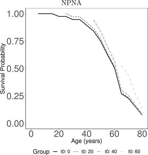
Dynamic landmark predictions of survival past age |$t$| given survival to age |$t_0$| in the COHORT study, |$t\geq t_0$|. Estimates are shown as a function of age (in years) for relatives who are male, mutation carriers whose proband had 46 CAG repeats. Result displayed is from the proposed nonparametric kernel Nelson-Aalen estimator (NPNA).
Figure S.2. of the Supplementary material available at Biostatistics online displays the predicted survival using the NPNA estimator to compare differences between carrier and non-carrier relatives (top-half), and differences between carrier males and females (bottom-half). The probability of survival for non-carriers was nearly one up until age 60, with a steady decrease thereafter. The carriers, however, had steadily decreasing probabilities of survival beginning at age 20 and rapidly decreasing thereafter. These differences underscore the insidious effect of genetic mutation on mortality. Mortality rates appeared similar for males and females (the 95% confidence bands for carrier males and females overlapped; see bottom-half of Figure S.2. of the Supplementary material available at Biostatistics online). The result agrees with earlier studies where gender did not significantly impact the mean survival time of HD patients (Harper, 1996).
5. Discussion
We developed a new nonparametric prediction model for mixture data that incorporates covariates and dynamic landmark prediction, and we showed how it improves prediction accuracy. There are several extensions of our work.
A straightforward extension is the incorporation of clinically important intermediate event information, such as hospitalization. The estimator |$\widehat S_j(t \mid t_0,z, w)$|, |$j=1,\ldots,m$|, in (2.1) can be adapted to incorporate the timing of intermediate events through |$W$|. Specifically, let |$M_i$| indicate the time of the intermediate event. Similar to the failure time |$T_i$|, |$M_i$| is subject to censoring and thus we may only observe |$M_i^* = \min(M_i, C_i, T_i)$| and |$\Delta_i^* = I(M_i \leq C_i)$|. Among individuals in |$\Omega_{t_0}=\{i:X_i>t_0\}$|, if |$M_i<t_0$| then |$M_i^* = M_i$|. That is, for those who have survived to |$t_0$| and are still under observation at |$t_0$|, it is known that |$C_i > t_0$| and thus if the intermediate event occurred before |$t_0$|, then it was observed. Therefore, when we condition on |$\Omega_{t_0}$|, we can re-define |$W_i$| as |$W_i(t_0) = \min(M_i, t_0)$| and thus, |$W_i(t_0)$| will be equal to |$t_0$| for those who have not yet experienced the intermediate event by |$t_0$| or equal to |$M_i^*$| for those who have experienced the intermediate event by |$t_0$|. Estimation of |${\boldsymbol F}(t \mid t_0, Z_i,W_i)$| then follows the procedure in Section 2, where |$W_i = W_i(t_0) = \min(M_i, t_0)$| and with or without an additional discrete covariate |$Z_i$|.
Another extension is with competing risks. In the HD study, one could be interested in different causes of death due to cardiovascular disease, pneumonia, or suicide (Sørensen and Fenger, 1992 ). To handle competing risks, we could re-define |${\boldsymbol F}(t\mid t_0,z,w)$| as a cumulative incidence function: |${\boldsymbol F}_j(t\mid t_0,z,w)$||$=\{F_{j1}(t\mid t_0,z,w),\ldots,F_{jp}(t\mid t_0,z,w)\}^T$| where |$ F_{jk}(t\mid t_0, z,w) = P(T\leq t, D= j \mid T> t_0, L=k, z, w)$| and |$D$| denotes the type of event that occurred where |$j=1,...,J$| and |$J$| is the number of distinct competing event types. Estimation would focus on a cause-specific version of cumulative hazard in (2.2) and for estimation of each event, individuals experiencing other events would be censored at the event time.
Other extensions apply to the HD example. In the kin-cohort study, mortality outcomes between relatives in the same family are correlated. One could account for this correlation using frailties that adjust for correlations between outcomes from family members. These frailties would be incorporated into our modified nonparametric kernel Nelson–Aalen estimator. We could also explicitly incorporate left truncation of failure times given that survival times for relatives is collected retrospectively and some of these relatives have died prior to the study onset. However, incorporating left truncation requires a new framework beyond the scope of this article.
In practice, it may be of interest to use the estimates obtained to test for differences in predictions at some time |$t$| or differences in the survival curves up to time |$t$| between two groups (e.g., carrier vs. non-carriers, or male carriers vs. female carriers). To test at a particular time |$t$| this difference, e.g., |$H_0: F_1(t|t_0, z, w) - F_2(t|t_0, z, w) = 0$|, we could perform a Wald-type test using |$\mathcal{Z}(t|t_0,z,w) = \{\widehat{F}_1(t|t_0, z, w) - \widehat{F}_2(t|t_0, z, w)\}/\widehat{\sigma}_{12}(t|t_0,z,w)$|. Here, |$k=1$| indicates carrier and |$k=2$| indicates non-carrier and |$\widehat{\sigma}_{12}(t|t_0,z,w)$| is an estimate of the standard error of the difference between |$\widehat{F}_1(t|t_0, z, w)$| and |$\widehat{F}_2(t|t_0, z, w)$| which we can obtain using our bootstrap samples. To compare survival curves, we could define the function |$\widehat{\mathcal{D}}_{12}(t|t_0, z, w) = \widehat{F}_1(t|t_0, z, w) - \widehat{F}_2(t|t_0, z, w)$| for |$t>t_0$| in some range |$\mathcal{T}$|, and calculate a simultaneous confidence band |$\{\widehat{\mathcal{D}}_{12}(t|t_0, z, w) \pm \widehat{c}_{\alpha}\widehat{\sigma}_{12}(t|t_0,z,w), t\in \mathcal{T}\}$| where |$\widehat{c}_{\alpha}$| is the |$(1-\alpha)$| empirical quantile of |$\sup_{t\in \mathcal{T}} || $||$ \widehat{\mathcal{D}}_{12}^{b}(t|t_0, z, w) - \widehat{\mathcal{D}}_{12}(t|t_0, z, w) || / \widehat{\sigma}_{12}(t|t_0,z,w), b=1,...,B \}$| where |$b$| indicates the bootstrap replication.
Our proposed approach does have some limitations. Because we use nonparametric kernel smoothing, we require a relatively large sample size and in particular, there must be adequate sample size within each |${\boldsymbol u}_j$| group. In settings with smaller sample sizes, parametric approaches may be more stable. Second, our proposed estimators were presented assuming covariates |$Z$| and |$W$| were univariate. Our method can extend to the multivariate case using, for example, a dimension reduction approach whereby a working model is used to reduce the multivariate covariate information into a single scalar summary. After this dimension reduction, our proposed approach could then be directly applied. Third, though we note that our method can incorporate information on time-dependent covariates, where |$Z$| and |$W$| are updated at the landmark time |$t_0$| resulting in |$Z(t_0)$| and |$W(t_0)$|, we do not have access to mixture data with time-dependent covariates and thus, are unable to illustrate this feature. However, this methodological development and the availability of software to implement these methods would allow others with such data to apply these methods. Fourth, the prediction accuracy using AUC and BS requires knowing the population identifier, which is only known in simulated data but not in practice. We thus cannot compute prediction accuracy for our HD study, but results from our simulation study suggest that our proposed estimator indeed has better prediction accuracy than competing methods.
6. Software
All R code is available at https://github.com/tpgarcia/landmix.
Supplementary material
Supplementary material is available at http://biostatistics.oxfordjournals.org.
Acknowledgments
Data from the COHORT study, which received support from HP Therapeutics, Inc., were used. We thank the Huntington Study Group COHORT investigators and coordinators who collected the data, and participants and their families who made this work possible.
Conflict of Interest: None declared.
Funding
The Huntington’s Disease Society of America Human Biology Project Fellowship, the National Institute of Neurological Disorders and Stroke (K01NS099343); and the National Institute of Diabetes and Digestive and Kidney Diseases (R21DK103118).
