


Summary
Pooling biomarker data across multiple studies allows for examination of a wider exposure range than generally possible in individual studies, evaluation of population subgroups and disease subtypes with more statistical power, and more precise estimation of biomarker-disease associations. However, circulating biomarker measurements often require calibration to a single reference assay prior to pooling due to assay and laboratory variability across studies. We propose several methods for calibrating and combining biomarker data from nested case–control studies when reference assay data are obtained from a subset of controls in each contributing study. Specifically, we describe a two-stage calibration method and two aggregated calibration methods, named the internalized and full calibration methods, to evaluate the main effect of the biomarker exposure on disease risk and whether that association is modified by a potential covariate. The internalized method uses the reference laboratory measurement in the analysis when available and otherwise uses the estimated value derived from calibration models. The full calibration method uses calibrated biomarker measurements for all subjects, including those with reference laboratory measurements. Under the two-stage method, investigators complete study-specific analyses in the first stage followed by meta-analysis in the second stage. Our results demonstrate that the full calibration method is the preferred aggregated approach to minimize bias in point estimates. We also observe that the two-stage and full calibration methods provide similar effect and variance estimates but that their variance estimates are slightly larger than those from the internalized approach. As an illustrative example, we apply the three methods in a pooling project of nested case–control studies to evaluate (i) the association between circulating vitamin D levels and risk of stroke and (ii) how body mass index modifies the association between circulating vitamin D levels and risk of cardiovascular disease.
1. Introduction
Combining data from multiple studies to maximize sample size has become a common strategy to quantify exposure-disease associations, including those where the exposure is a biomarker. Increased sample sizes facilitate subgroup and tumor subtype analyses, allow more precise estimation of the biomarker exposure effect over a wider range of biomarker measurements, and avoid issues related to data sparsity (Key and others, 2010; Smith-Warner and others, 2006). The increase in the use of pooling consortia over time reflects the availability and advantages of big data in epidemiology and its promises to improve quantification of disease risk factors. Note that we use the term pooling throughout this article to refer to combination of data from individual participants and not physical specimen combination. Here, we define biomarkers as measurable indicators of health at the molecular, biochemical, or cellular level (Key and others, 2010). Examples include proteins, antibodies, hormones, and lipids. Many consortia have analyzed biomarker-disease associations, including the Endogenous Hormones, Nutritional Biomarkers, and Prostate Cancer Collaborative Group (Key and others, 2010), the COPD Biomarkers Qualification Consortium Database (Tabberer and others, 2017), and the Circulating Biomarkers and Breast and Colorectal Cancer Consortium (McCullough and others, 2018), among others. The participating cohorts in many consortia have employed nested case–control studies using individual or frequency matching to improve efficiency.
An important consideration when conducting pooled analyses of biomarker measurements from different studies is whether the measurements differ across studies due to real differences in the underlying populations or due to usage of different assays, kits, or laboratories in some or all studies. This consideration is particularly important when samples in the pooled analysis were assayed at different laboratories with different assays at different times. Examples of biomarkers with highly variable measurements across assays and laboratories include estradiol, testosterone, and insulin-like growth factor 1 (Key and others, 2010). Measurements of circulating 25-hydroxyvitamin D (25(OH)D) also vary up to 40% between laboratories and assays (Lai and others, 2012).
For consortial projects of biomarkers that do not use a single assay and laboratory, investigators must address potential between-study variation in biomarker measurements. Critically, to quantify risk associated with per-unit increases in the biomarker, a common metric for the biomarker data must be used in each of the contributing studies. One strategy used to harmonize biomarker measurements involves study-specific calibration models. In this method, a random subset of biospecimens from each study is reassayed at a designated reference laboratory. A study-specific calibration model is estimated in each study between the original “local” laboratory measurements and reference laboratory measurements. The resulting calibration equation is then used to estimate the reference laboratory biomarker measurement from the local laboratory measurement for all cases and controls in the individual study. Following the calibration procedure, the harmonized biomarker measurements can be modeled using categories defined by absolute concentrations, consortium-wide quantiles, or continuously. In practice, re-assayed biospecimens are typically selected at random from controls in each study owing to concerns about the availability of case biospecimens (Sloan and others, 2019).
Two major classes of methods exist for analyzing data pooled from multiple studies, namely the two-stage approach and the aggregated approach (Debray and others, 2013; Smith-Warner and others, 2006). Under the two-stage method, investigators complete study-specific analyses using standardized criteria in the first stage followed by meta-analysis in the second stage. In the aggregated approach, investigators combine harmonized data from all studies into a single dataset before performing statistical analyses on the combined dataset. Sloan and others (2019) developed pooling methodology for cohort studies and subdivided the aggregated approach into the internalized and full calibration approach. The internalized method uses the reference laboratory measurement in the analysis when available and the calibrated measurement otherwise. In contrast, the full calibration method uses calibrated biomarker measurements exclusively for all subjects regardless of the availability of reference laboratory measurements. In this article, we derive these approaches under the paradigm of nested case–control studies, allowing the potential inclusion of a biomarker–covariate interaction term.
The methods developed here are gnostic to the type of assay being used or biomarker being measured so long as investigators have access to reference assay measurements for a subset of individuals at each local laboratory and can model the relationship between reference laboratory measurements and local laboratory measurements. Variation in the assays or laboratories are captured in these study-specific models.
We can equivalently view pooled and calibrated biomarker data as a covariate measurement error problem. If we treat the reference and local laboratory measurements as the true and surrogate biomarker values, respectively (Carroll and others, 2006), we can envision each study-specific calibration model as a different measurement error model. We leverage an existing strategy in the measurement error literature, namely regression calibration (Carroll and others, 2006; Rosner and others, 1990), to form the basis of our methods. Although each of our methods are classified as a two-stage or aggregated approach, each utilizes concepts underlying regression calibration.
In this article, we propose calibration methods for pooled biomarker data from nested case–control studies that allow inference on the main effect of the biomarker in addition to biomarker–covariate interaction terms. Section 2 presents the models and statistical methods. Section 3 compares the methods via simulation and considers the inclusion of a covariate–biomarker interaction term. Section 4 illustrates the methods in examples involving 25(OH)D data pooled from the Nurses’ Health Study I (NHS1), Nurses’ Health Study II (NHS2), and Health Professionals Follow-up Study (HPFS) for stroke and cardiovascular disease (CVD) outcomes. Section 5 discusses our results.
2. Methods
2.1. Model and approximate conditional likelihood
Let |$s=1,\dots,S$| index the studies contributing to the pooled analysis, where the first |$Q$| studies require biomarker calibration. For presentational simplicity, we focus on |$1:m_s$| matching; it is straightforward to extend the methods to settings where multiple cases exist in some or all strata. Allow subscript |$i$| to index individuals within stratum |$j$| of study |$s$| such that |$i=m_s$| corresponds to the case and |$i=0,1,\dotsc,m_s-1$| corresponds to the matched controls.
Let |$Y_{sji}$| be the binary disease outcome, |$X_{sji}$| be the biomarker exposure measurement from the reference laboratory, |$W_{sji}$| be the biomarker exposure measurement from the local laboratory, and |$\boldsymbol{Z}_{sji}$| be a vector of other covariates. Without further specification, all vectors are column vectors. We assume |$X_{sji}$| is not available for all subjects due to the usage of a local laboratory to obtain biomarker measurements in at least one study. However, we assume |$W_{sji}$| is available for all subjects in studies obtaining measurements from local laboratories. Using |$W_{sji}$| as a direct substitute for |$X_{sji}$| in the analysis will lead to biased estimates of the biomarker–outcome relationship if measurement variability exists across the study laboratories and the biomarker is modeled using common absolute cutpoints across studies or continuously.
To estimate the biomarker exposure effect under the aggregated approach, we develop a likelihood-based method. The conditional logistic regression model for the biomarker–disease association is
where |$\beta_{0sj}$| is a stratum-specific intercept and |$\boldsymbol{\beta}_z$| is a covariate effect vector. We desire point and interval estimates for |$\beta_x$|. For nested case–control studies using incidence density sampling, |$\beta_x$| is the log relative risk (RR) describing the biomarker–disease association (Prentice and Breslow, 1978).
Let vectors |$\boldsymbol{X}_{sj}, \boldsymbol{W}_{sj}, \boldsymbol{Y}_{sj}$|, and matrix |$\boldsymbol{Z}_{sj}$| contain their respective measurements from all individuals in stratum |$j$| of study |$s$|. The conditional likelihood (Breslow and others, 1978) is
The conditional likelihood contribution cannot be computed for studies using a local laboratory because |$X_{sji}$| is unavailable for individuals outside the calibration subset. Under a surrogacy assumption, we derive an approximate conditional likelihood below that uses an estimate of |$X_{sji}$| in place of |$X_{sji}$| itself. The surrogacy assumption states that |$f(\boldsymbol{Y}_{sj} \,{|}\, \boldsymbol{X}_{sj}, \boldsymbol{Z}_{sj}, \boldsymbol{W}_{sj}, \sum_{i=0}^{m_s} Y_{sji}=1) = f(\boldsymbol{Y}_{sj} \,{|}\, \boldsymbol{X}_{sj}, \boldsymbol{Z}_{sj}, \sum_{i=0}^{m_s} Y_{sji}=1)$|; in essence the biomarker measurement from the reference laboratory provides at least as much information about the likelihood of disease as the analogous measurement from the local laboratory, conditional on the covariates and matching scheme.
Under aggregation, the likelihood contribution from a stratum with only local laboratory biomarker measurements is
where the surrogacy assumption is used in the third line. A second order Taylor series approximation about |$\boldsymbol{X}_{sj}$| with respect to |$E[\boldsymbol{X}_{sj}| \boldsymbol{W}_{sj}, \boldsymbol{Z}_{sj}, \sum_{i=0}^{m_s} Y_{sji}=1]$| yields the approximate contribution by stratum |$j$| of study |$s$|, namely
where |$\tilde{X}_{sji}-\tilde{X}_{sjm_s}=E[X_{sji}| W_{sji}, \boldsymbol{Z}_{sji}, \sum_{i=0}^{m_s} Y_{sji}=1]-E[X_{sjm_s}| W_{sjm_s}, \boldsymbol{Z}_{sjm_s}, \sum_{i=0}^{m_s} Y_{sji}=1]$|. This approximate conditional likelihood performs best when the elements in the variance–covariance matrix |$Var(\boldsymbol{X}_{sj}|\boldsymbol{W}_{sj},\boldsymbol{Z}_{sj},\sum_{i=0}^{m_s} Y_{sji}=1)$| are small (i.e. there is minimal noise in the relationship between |$X_{sji}$| and |$W_{sji}$| conditional on the covariates and matching scheme) or when the association between |$Y_{sji}$| and |$X_{sji}$| is not strong. Further details about these conditions and the full derivation of the approximate conditional likelihood are available in Section 1 of the supplementary material available at Biostatistics online. The presence of |$E[X_{sji}|W_{sji},\boldsymbol{Z}_{sji},\sum_{i=0}^{m_s} Y_{sji}=1]$| in the approximate conditional likelihood contribution |$\tilde{l}_{sj}$| motivates the construction of calibration models.
2.2. Calibration model
To evaluate |$\tilde{l}_{sj}$|, we formulate study-specific calibration models among studies using a local laboratory to measure the biomarker of interest. In these studies, we estimate a calibration model from a subset of controls who have both reference and local laboratory measurements available. The resulting model quantifies the relationship between |$X_{sji}$| and |$W_{sji}$| and is used to estimate the reference laboratory measurement among individuals with only a local laboratory measurement.
For presentational simplicity, we drop |$\boldsymbol{Z}_{sji}$| from the calibration models such that |$E[X_{sji}|W_{sji}, \boldsymbol{Z}_{sji},\sum_{i=0}^{m_s} Y_{sji}=1] \approx E[X_{sji}|W_{sji},\sum_{i=0}^{m_s} Y_{sji}=1]$|. In words, this approximation states that conditional on the matching scheme, the relationship between the reference and local laboratory measurements is minimally impacted by other covariates. Previous work demonstrates that, when not conditional on |$\sum_{i=0}^{m_s} Y_{sji}=1$|, omitting |$\boldsymbol{Z}_{sji}$| has a negligibly small impact on the resulting calibration models so long as |$\boldsymbol{Z}_{sji}$| is not very strongly correlated with |$X_{sji}$| (Sloan and others, 2019). The additional condition, |$\sum_{i=0}^{m_s} Y_{sji}=1$|, does not change this conclusion. Nonetheless, our methods can accommodate additional covariates in the calibration model if investigators believe that they are necessary to model the relationship between |$X_{sji}$| and |$W_{sji}$|.
We assume a linear relationship between the reference and local laboratory measurements among the matched cases and controls such that
where |$a_s$| and |$b_s$| are the calibration parameters. Note that model (2.2) indicates that the calibration parameters are study-specific and invariant over the strata of each study. The assumption of invariance over strata could be relaxed by instead assuming |$E[X_{sji}|W_{sji},\boldsymbol{U}_{sji},\sum_{i=0}^{m_s} Y_{sji}=1] = a_s + b_s W_{sji} + \boldsymbol{c}^T_{s} \boldsymbol{U}_{sji}$|, where |$\boldsymbol{U}_{sji}$| is a vector that may contain some or all of the matching factors. Previous work suggests that the simple linear model in (2.2) is appropriate and sufficient for the relationship between 25(OH)D measurements taken from different laboratories (Gail and others, 2016; Sloan and others, 2019).
Due to concerns about the availability of case biospecimens for reassay at the reference laboratory, the calibration models in (2.2) are typically fit among controls only, i.e. |$\hat{E}[X_{sji}|W_{sji},Y_{sji}=0]=\hat{a}_{s,co}+\hat{b}_{s,co} W_{sji}$|. While |$\hat{a}_{s,co}$| and |$\hat{b}_{s,co}$| are generally not consistent estimators of |$a_s$| and |$b_s$|, we can show that the controls-only parameters approximate the parameters of model (2.2) under most circumstances. Specifically, under multivariate normality of |$(\boldsymbol{X}_{sj},\boldsymbol{W}_{sj})$|, |$\hat{a}_{s,co}$| converges to a value close to |$a_s$| when |$E[\boldsymbol{X}_{sj}|\sum_{i=0}^{m_s} Y_{sji}=1] \approx E[\boldsymbol{X}_{sj}|\boldsymbol{Y}_{sj}=\boldsymbol{0}]$| and |$Var(\boldsymbol{X}_{sj}|\sum_{i=0}^{m_s} Y_{sji}=1) \approx Var(\boldsymbol{X}_{sj}|\boldsymbol{Y}_{sj}=\boldsymbol{0})$|, and |$\hat{b}_{s,co}$| converges to a value close to |$b_s$| when |$Var(\boldsymbol{X}_{sj}|\sum_{i=0}^{m_s} Y_{sji}=1) \approx Var(\boldsymbol{X}_{sj}|\boldsymbol{Y}_{sj}=\boldsymbol{0})$|. Alternatively, if the biomarker effect is not too large, then |$\hat{a}_{s,co}$| and |$\hat{b}_{s,co}$| also converge to values close to |$a_s$| and |$b_s$|. Further details are available in Section 2 of the supplementary material available at Biostatistics online. We also show the approximation for a single study via simulation using parameters listed in Section 3.1. Over 1000 simulation replicates, the mean percent bias of the estimated parameters in (2.2) is close to zero while the controls-only calibration parameter estimates are only depressed up to 12% for very large RRs (Figure 1 of supplementary material available at Biostatistics online). The intercept estimates are typically more biased than the slope estimates, and the downward bias is more pronounced for increasingly non-null RRs. Simulations for other values of |$a_s$| and |$b_s$| (not shown here) demonstrate that these patterns are invariant to the specific values of the calibration parameters.
Let |$\tilde{X}_{sji}$| be the estimated biomarker measurement used in place of |$X_{sji}$| in the aggregated analysis. Its value depends on the chosen calibration approach and availability of the reference laboratory measurement. For studies using the reference laboratory for all biomarker measurements, no calibration occurs and |$\tilde{X}_{sji}=X_{sji}$| for all study participants. For studies using a local laboratory, the full calibration and internalized methods are defined as follows:
where |$\hat{E}[X_{sji}|W_{sji}, Y_{sji}=0]=\hat{a}_{s,co}+\hat{b}_{s,co} W_{sji}$|. The pooled analysis uniformly applies one of these methods to all studies using local laboratories.
The biomarker measurements appear in the likelihood via the difference |$X_{sji}-X_{sjm}$|. For the full calibration method, the calibrated difference simplifies to |$\tilde{X}_{sji}-\tilde{X}_{sjm}=\hat{b}_{s,co}(W_{sji}-W_{sjm})$| for all observations. Consequently, bias in the intercept |$\hat{a}_{s,co}$| does not impact the |$\beta_x$| estimator under the full calibration method. In contrast, for observations in the calibration study subset under the internalized method, |$\tilde{X}_{sji}-\tilde{X}_{sjm}= X_{sji} - (\hat{a}_{s,co}+\hat{b}_{s,co}W_{sji})$|. Thus, bias in both the intercept and slope estimates |$\hat{a}_{s,co}$| and |$\hat{b}_{s,co}$| induces bias in the internalized method |$\beta_x$| estimate. We will see in simulation studies that the relative performance of the internalized, full calibration, and two-stage methods is impacted by the size of the calibration subset.
2.3. Parameter estimation under aggregated approach
Recall that |$Q$| studies require biomarker calibration. Define |$\boldsymbol{\beta}=[\beta_x, \boldsymbol{\beta}_z]$|, |$\boldsymbol{a}=[a_1,\dotsc , a_Q]$|, and |$\boldsymbol{b}=[b_1 , \dotsc ,b_Q]$| such that our target of estimation is |$\boldsymbol{\theta}=[\boldsymbol{a} , \boldsymbol{b} , \boldsymbol{\beta}]$|. We define estimating equations |$ [\boldsymbol{\psi}_{\boldsymbol{a}} , \boldsymbol{\psi}_{\boldsymbol{b}} , \psi_{\beta_x} , \boldsymbol{\psi}_{\boldsymbol{\beta}_z} ] = \boldsymbol{0}$|, where |$\boldsymbol{\psi}_{\boldsymbol{a}}$|, |$\boldsymbol{\psi}_{\boldsymbol{b}}$|, |$\psi_{\beta_x}$|, and |$\boldsymbol{\psi}_{\boldsymbol{\beta}_z}$| are approximately unbiased estimating functions for their respective parameters (see Section 3 of the supplementary material available at Biostatistics online).
Estimates of |$\boldsymbol{\beta}$| are obtained through a two-step process involving the pseudo maximum likelihood estimation method (Gong and Samaniego, 1981). We first estimate the calibration parameters |$\hat{\boldsymbol{a}}$| and |$\hat{\boldsymbol{b}}$| by fitting the linear regression calibration models. We then obtain |$\hat{\boldsymbol{\beta}}$| using pseudo-maximum conditional likelihood estimation over the set of estimating equations |$[\psi_{\beta_x}(\hat{\boldsymbol{a}},\hat{\boldsymbol{b}}) , \boldsymbol{\psi}_{\boldsymbol{\beta}_z}(\hat{\boldsymbol{a}},\hat{\boldsymbol{b}}) )]=\boldsymbol{0}$|, where instances of |$\boldsymbol{a}$| and |$\boldsymbol{b}$| have been replaced with their estimates. Since the estimating equations for |$\boldsymbol{\beta}$| are with respect to |$\tilde{l}_{sj}$| where |$\hat{\boldsymbol{a}}$| and |$\hat{\boldsymbol{b}}$| are treated as known, the estimates are not the same as those obtained from maximizing a joint likelihood, which is the product of the likelihood for |$\boldsymbol{\beta}$| and the likelihood for |$\boldsymbol{a}$| and |$\boldsymbol{b}$|.
We must account for uncertainty in the estimation of |$\hat{\boldsymbol{a}}$| and |$\hat{\boldsymbol{b}}$| when estimating |$\widehat{Var}(\hat{\boldsymbol{\beta}})$|. As a result, we use the sandwich variance formulas over the entire set of estimating equations. The appropriate diagonal terms of the sandwich variance matrix provide variance estimates for |$\hat{\boldsymbol{\beta}}$| (see Section 4 of the supplementary material available at Biostatistics online).
2.4. Two-stage approach
The two-stage approach for pooled data uses regression calibration, a broadly applicable method initially developed in the measurement error literature, to adjust for calibration in the first stage study-specific analyses (Carroll and others, 2006; Rosner and others, 1990; Spiegelman and others, 1997, 2001). The second stage combines these estimates using fixed effects meta-analysis.
Regression calibration for cohort studies using standard logistic regression has been robustly developed by Rosner, Spiegelman, and Willett, among others ( Carroll and others, 2006; Rosner and others, 1990). However, there has been less focus on the application of regression calibration to the setting of matched data with conditional logistic regression. Using simulation studies and randomly sampled internal validation studies, McShane and others (2001) tested the performance of the regression calibration point estimate formula to obtain |$\beta_x$| point estimates under conditional logistic regression. Their results demonstrated that regression calibration performed well for exposure effects that were not too strong. Effectively, the matched nature of the data is ignored in the calibration step but accounted for in the conditional logistic regression step. Further simulations by Guolo and Brazzale (2008) extended regression calibration to the matched data setting. However, neither manuscript provided simulations specific to the setting of controls-only calibration data, which we consider analytically in Section 2 and via simulation in Section 3 of the supplementary material available at Biostatistics online.
The assumptions required by regression calibration for matched case–control studies are similar to cohort studies, including: (i) the surrogacy assumption defined in section 2.1 and (ii) the noise in the calibration model is moderate and/or the association between |$Y$| and |$X$| is not too strong.
We briefly describe the two-stage method and its implementation of regression calibration. For studies using the reference laboratory for all biomarker measurements, we directly obtain effect and variance estimates from a conditional logistic regression model. Among studies whose biomarkers were measured by a local laboratory, we estimate |$\hat{\beta}_{x,q}$|, the adjusted effect estimate in study |$q$| obtained from the regression calibration method such that
where |$\hat{b}_q$| is obtained from the calibration study and |$\hat{\beta}_{w,q}$| and |$\widehat{Var}(\hat{\beta}_{w,q})$| are the naive estimates from a conditional logistic regression model fit using all local laboratory measurements of individuals in study |$q$|. Formula (2.3) for |$\widehat{Var}(\hat{\beta}_{x,q})$| leverages the fact that the conditional logistic regression estimates, |$\hat{\beta}_{w,q}$|, and the calibration parameter estimate, |$\hat{b}_q$| are uncorrelated asymptotically (proof in Section 5 of supplementary material available at Biostatistics online). Fixed-effects meta-analysis combines the study-specific estimates using inverse variance weights to obtain a final effect and variance estimate for |$\hat{\beta}_x$|.
2.5. Two-stage method for models with an interaction term
Suppose |$V_{sji}$| is a covariate whose interaction with |$X_{sji}$| is of interest. The conditional logistic regression model with an interaction term between |$X_{sji}$| and |$V_{sji}$| is
For the aggregated methods, the development of an approximate conditional likelihood involving an interaction term follows similarly to section 2.1 (see Section 1 of the supplementary material available at Biostatistics online). However, the two-stage method for models involving interaction terms must be modified to address inference for |$(\beta_x, \beta_v, \beta_{xv})$|. In the |$q^{th}$| study with local laboratory measurements, suppose we fit the following naive model using all local laboratory biomarker measurements:
Like before, assume we obtain study-specific estimates |$\hat{a}_q$| and |$\hat{b}_q$| by fitting the linear model |$E[X_{qji}|W_{qji},Y_{qji}=0]=\hat{a}_q + \hat{b}_q W_{qji}$| in each calibration subset. We derive a modified form of regression calibration to obtain adjusted point estimates of |$\beta_x$|, |$\beta_v$|, and |$\beta_{xv}$| in each study using a local laboratory such that
The full derivation of the point and variance estimates can be found in Section 6 of the supplementary material available at Biostatistics online. Of note, the formulas for the point and variance estimates of |$\hat{\beta}_{x,q}$| follow similarly to the case of no interaction term. The estimates for |$\hat{\beta}_{xv,q}$| follow similarly to |$\hat{\beta}_{x,q}$|, and |$\hat{\beta}_{v,q}$| has a slightly more complex adjustment given the interaction term between |$X_{sji}$| and |$V_{sji}$|.
3. Simulations
3.1. Model without an interaction term
We simulated 1:1 matched case–control data by generating data for each stratum and then selecting a case and control at random from each stratum. Let |$e_{sji}$| be the error term in the linear regression of |$X_{sji}$| on |$W_{sji}$|. We assumed joint multivariate normality of |$(X_{sji}, W_{sji}, e_{sji})$| and generated data such that
This formulation induces |$E[X_{sji}|W_{sji}]=a_s+b_sW_{si}$| and |$Cov(W_{sji}, e_{sji})=0$|. We assumed that the stratum-specific intercepts |$\beta_{0sj}$| were normally distributed such that |$\beta_{0sj} \sim N(\mu_{\beta_0},\sigma^2_{\beta_0})$|, and used a simple risk model without covariates, |$\textrm{logit}(P(Y_{sji}=1|X_{sji})) = \beta_{0sj} + \beta_x X_{sji}$|.
We set |$\mu_x=0$|, |$\sigma_x^2=1$|, |$\mu_{\beta_0}=-1$| and |$\sigma^2_{\beta_0}$|=0.01. We assumed four studies contributed to the final analysis, each with 1000 total subjects (or 500 case–control pairs) and 100 calibration participants, and assigned calibration parameters |$\boldsymbol{a}=[-3,1,-1,3]$|, and |$\boldsymbol{b}=[0.5,0.75,1.25,1.5]$|. These parameters were selected to mirror parameters chosen by Sloan and others (2019), whose values were chosen to display a variety of potential relationships between the local and reference laboratory measurements, including those in our real example in Section 4. We completed 1000 simulation replicates at six RRs, including |$(1.25, 1.5, 1.75, 2, 2.25, 2.5)$|.
We compared the two aggregated procedures (i.e. full calibration and internalized methods) and the two-stage approach with regard to mean percent bias of |$\hat{\beta}_x$| over the simulation replicates, mean squared error (MSE) of |$\hat{\beta}_x$|, and coverage rate, defined as the proportion of simulation replicates whose 95% confidence intervals covered the true |$\beta_x$|. For comparison, we also included a naive method that did not calibrate the measurements from the local laboratories and used |$W_{sji}$| in the logistic regression. We assumed that increasing levels of the biomarker increased disease risk, although similar results were obtained when the biomarker instead lowered disease risk (not shown). We provide tables of results in the main paper and include graphs of the mean percent bias estimates from these tables in Section 7 of the supplementary material available at Biostatistics online.
As shown in Table 1, the naive method performed poorly over all effects and underscored the need for calibration. At every RR considered, the percent bias of the naive estimate exceeded |$-$|27% and the corresponding coverage rates were less than 40%. The full calibration method estimates were consistently less biased than the internalized method estimates. Over the range of RRs considered, the internalized estimate was biased downward by approximately 3–4%, while the full calibration estimate was biased by less than 1%. For RRs of at least 2.0, the coverage rate under the internalized method decreased to 90–91% due to depression of point estimates. In contrast, the coverage rates of the full calibration and two-stage methods ranged from 93% to 96%. The two-stage approach generally performed comparably to the full calibration method with regards to percent bias in the RR estimate, MSE, and coverage rate.
Comparison of operating characteristics for |$\beta_x$| under the model |$\textrm{logit}(P(Y_{sji}=1|X_{sji})) = \beta_{0sj} + \beta_xX_{sji}$|, for naive (|$\hat{\beta}_{N}$|), internalized (|$\hat{\beta}_{IN}$|), full calibration (|$\hat{\beta}_{FC}$|), and two-stage (|$\hat{\beta}_{TS}$|) methods
| Mean percent bias (SE) | MSE | Coverage rate | ||||||||||||
|---|---|---|---|---|---|---|---|---|---|---|---|---|---|---|
| |$\beta_x$| | |$\hat{\beta}_N$| | |$\hat{\beta}_{IN}$| | |$\hat{\beta}_{FC}$| | |$\hat{\beta}_{TS}$| | |$\hat{\beta}_N$| | |$\hat{\beta}_{IN}$| | |$\hat{\beta}_{FC}$| | |$\hat{\beta}_{TS}$| | |$\hat{\beta}_N$| | |$\hat{\beta}_{IN}$| | |$\hat{\beta}_{FC}$| | |$\hat{\beta}_{TS}$| | ||
| log(1.25) | |$-$|29.4 (0.029) | |$-$|3.1 (0.037) | 0.1 (0.038) | |$-$|0.8 (0.038) | 0.0051 | 0.0014 | 0.0014 | 0.0014 | 0.37 | 0.96 | 0.95 | 0.96 | ||
| log(1.50) | |$-$|29.0 (0.032) | |$-$|3.2 (0.040) | 0.0 (0.042) | |$-$|0.9 (0.042) | 0.0149 | 0.0018 | 0.0018 | 0.0018 | 0.05 | 0.95 | 0.94 | 0.95 | ||
| log(1.75) | |$-$|28.6 (0.035) | |$-$|3.5 (0.043) | |$-$|0.1 (0.045) | |$-$|1.0 (0.045) | 0.0269 | 0.0023 | 0.0021 | 0.0021 | 0.01 | 0.93 | 0.94 | 0.95 | ||
| log(2.00) | |$-$|28.2 (0.039) | |$-$|3.5 (0.049) | 0.0 (0.051) | |$-$|1.0 (0.051) | 0.0396 | 0.0030 | 0.0027 | 0.0027 | 0.00 | 0.91 | 0.93 | 0.93 | ||
| log(2.25) | |$-$|28.0 (0.042) | |$-$|3.6 (0.052) | |$-$|0.1 (0.055) | |$-$|1.1 (0.055) | 0.0532 | 0.0036 | 0.0030 | 0.0031 | 0.00 | 0.90 | 0.94 | 0.94 | ||
| log(2.50) | |$-$|27.9 (0.044) | |$-$|3.9 (0.055) | |$-$|0.3 (0.058) | |$-$|1.3 (0.058) | 0.0671 | 0.0043 | 0.0034 | 0.0035 | 0.00 | 0.90 | 0.96 | 0.94 | ||
Percent bias and MSE are computed by |$(\hat{\beta}-\beta)/\beta$| and |$(\beta - \hat{\beta})^2$|, respectively and the reported value is the average over 1000 simulations. Standard error is the square root of the empirical variance over all replicates. The coverage rate is the proportion of simulations whose estimated 95% confidence intervals covered the true effect |$\beta_x$|.
We also performed simulations that fixed the total sample size at 1000 participants while varying the calibration subset size between 30, 50, and 150 subjects (or 3%, 5%, and 15% participation rates, respectively). As shown in Figure 1, at all calibration study sizes, the full calibration method offered nearly unbiased point estimates. With larger calibration study sizes, the MSEs decreased as a result of the improvement in efficiency. However, the internalized method estimates experienced increasing downward bias as the proportion of subjects participating in the calibration subset increased owing to increasingly differential calibration of cases and controls. As calibration study size increased, the two-stage method point estimates were increasingly less biased with decreasing MSEs owing to the improved bias and efficiency of calibration parameters.
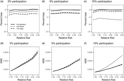
Comparison of methods as number of participants in the calibration study increases. The number of subjects in each study remains fixed at 1000, or equivalently, 500 case–control pairs. The calibration study participation rates considered are 3%, 5%, and 15%, or 30, 50, and 150 individuals, respectively. Panels a-c depict the percent bias of the parameter estimate while panels d-f display the MSE of the estimate.
3.2. Model with an interaction term
For the simulations involving a model with an interaction term, we also generated |$V_{sji}$| in the multivariate normal model for each stratum such that
where |$\mu_{ws} = (\mu_x-a_s)/b_s$|, |$\sigma_{wvs} = Cov(W_{sji},V_{sji})$|, and |$\sigma_{ws}^2 =(\sigma_x^2-\sigma^2_e)/b_s^2$|. We again used 1:1 matching and omitted other covariates such that the risk model was |$\text{logit}(P(Y_{si}=1|X_{sji},V_{sji})) = \beta_{0sj} + \beta_x X_{sji} + \beta_v V_{sji} + \beta_{xv} X_{sji}V_{sji}$|. Like before, we assumed four studies contributed to the analysis, each with 1000 total subjects and 100 individuals in the calibration subset. We set |$\mu_x=\mu_v=0$|, |$\sigma^2_x=\sigma_v^2=1$|, |$\boldsymbol{a}=(-3,1,-1,3)$|, |$\boldsymbol{b}=(0.5, 0.75, 1.25, 1.5)$|, and |$\text{Corr}(X_{sji},V_{sji})=0.2$|, which in turn induced |$\sigma_{wvs}$| for each study. We considered the same range of RRs for the main effect of the biomarker measurement and also chose four combinations of |$(\beta_{v},\beta_{xv})$| to address all possible qualitative effects of the covariate and interaction term, including |$(\exp(\beta_v),\exp(\beta_{xv})) \in [(0.8,0.8),(0.8,1.2),(1.2,0.8),(1.2,1.2)]$|. The simulation results for |$(\exp(\beta_v),\exp(\beta_{xv}))=(1.2,1.2)$| are reported in Table 2 while the results for |$(\exp(\beta_v),\exp(\beta_{xv})) \in [(0.8,1.2),(1.2,0.8),(1.2,1.2)]$| are presented in Section 7 of the supplementary material available at Biostatistics online.
Comparison of operating characteristics for (|$\beta_x$|,|$\beta_v$|,|$\beta_{xv}$|) for naive (N), internalized (IN), full calibration (FC), and two-stage (TS) methods under the model |$\text{logit}(P(Y_{sji}=1|X_{sji}, V_{sji}, \boldsymbol{Z}_{sji}))= \beta_{0sj} + \beta_xX_{sji}+\beta_vV_{sji}+\beta_{xv}X_{sji}V_{sji}$|, with |$(\exp(\beta_v),\exp(\beta_{xv}))=(1.2,1.2)$|
| Percent bias (SE) of |$\beta_x$| | MSE of |$\beta_x$| | Coverage rate of |$\beta_x$| | ||||||||||||
|---|---|---|---|---|---|---|---|---|---|---|---|---|---|---|
| |$\beta_x$| | N | IN | FC | TS | N | IN | FC | TS | N | IN | FC | TS | ||
| |$\log(0.5)$| | |$-$|25.8 (0.036) | |$-$|2.9 (0.045) | 0.9 (0.048) | 0.4 (0.048) | 0.0342 | 0.0023 | 0.0023 | 0.0023 | 0.00 | 0.95 | 0.96 | 0.96 | ||
| |$\log(0.8)$| | |$-$|29.4 (0.031) | |$-$|2.7 (0.037) | 0.6 (0.039) | 0.2 (0.039) | 0.0050 | 0.0015 | 0.0015 | 0.0015 | 0.41 | 0.96 | 0.96 | 0.95 | ||
| |$\log(1.2)$| | |$-$|28.6 (0.030) | |$-$|2.8 (0.037) | 0.3 (0.038) | |$-$|0.1 (0.038) | 0.0038 | 0.0014 | 0.0015 | 0.0014 | 0.54 | 0.96 | 0.96 | 0.96 | ||
| |$\log(1.5)$| | |$-$|27.6 (0.032) | |$-$|2.8 (0.041) | 0.4 (0.043) | |$-$|0.2 (0.043) | 0.0140 | 0.0018 | 0.0018 | 0.0018 | 0.06 | 0.96 | 0.95 | 0.95 | ||
| |$\log(2.0)$| | |$-$|25.7 (0.040) | |$-$|2.6 (0.048) | 0.9 (0.050) | 0.8 (0.050) | 0.0333 | 0.0026 | 0.0026 | 0.0026 | 0.00 | 0.95 | 0.96 | 0.95 | ||
| |$\log(2.5)$| | |$-$|23.4 (0.045) | |$-$|2.5 (0.054) | 1.4 (0.057) | 1.1 (0.057) | 0.0478 | 0.0034 | 0.0035 | 0.0034 | 0.00 | 0.96 | 0.96 | 0.95 | ||
| Percent bias (SE) of |$\beta_v$| | MSE of |$\beta_v$| | Coverage rate of |$\beta_v$| | ||||||||||||
|---|---|---|---|---|---|---|---|---|---|---|---|---|---|---|
| |$\beta_x$| | N | IN | FC | TS | N | IN | FC | TS | N | IN | FC | TS | ||
| |$\log(0.5)$| | |$-$|26.9 (0.035) | |$-$|6.5 (0.034) | |$-$|1.0 (0.035) | |$-$|1.0 (0.035) | 0.0019 | 0.0012 | 0.0012 | 0.0012 | 0.88 | 0.96 | 0.95 | 0.95 | ||
| |$\log(0.8)$| | |$-$|15.6 (0.034) | |$-$|2.7 (0.033) | |$-$|0.9 (0.034) | |$-$|1.0 (0.034) | 0.0014 | 0.0011 | 0.0011 | 0.0011 | 0.93 | 0.95 | 0.95 | 0.94 | ||
| |$\log(1.2)$| | |$-$|0.8 (0.033) | 1.5 (0.033) | 0.3 (0.033) | 0.3 (0.033) | 0.0011 | 0.0011 | 0.0011 | 0.0011 | 0.95 | 0.95 | 0.95 | 0.95 | ||
| |$\log(1.5)$| | 5.9 (0.034) | 3.1 (0.033) | 0.3 (0.033) | 0.2 (0.033) | 0.0012 | 0.0011 | 0.0011 | 0.0011 | 0.95 | 0.96 | 0.96 | 0.96 | ||
| |$\log(2.0)$| | 12.1 (0.035) | 5.4 (0.035) | 0.6 (0.035) | 0.4 (0.035) | 0.0013 | 0.0012 | 0.0012 | 0.0012 | 0.94 | 0.96 | 0.96 | 0.96 | ||
| |$\log(2.5)$| | 15.0 (0.035) | 7.6 (0.037) | 1.3 (0.037) | 1.2 (0.037) | 0.0015 | 0.0014 | 0.0014 | 0.0014 | 0.94 | 0.95 | 0.95 | 0.95 | ||
| Percent bias (SE) of |$\beta_{xv}$| | MSE of |$\beta_{xv}$| | Coverage rate of |$\beta_{xv}$| | ||||||||||||
|---|---|---|---|---|---|---|---|---|---|---|---|---|---|---|
| |$\beta_x$| | N | IN | FC | TS | N | IN | FC | TS | N | IN | FC | TS | ||
| |$\log(0.5)$| | |$-$|82.8 (0.011) | 1.3 (0.042) | 2.3 (0.043) | 1.6 (0.043) | 0.0063 | 0.0018 | 0.0019 | 0.0018 | 0.00 | 0.95 | 0.95 | 0.96 | ||
| |$\log(0.8)$| | |$-$|88.7 (0.010) | 0.4 (0.038) | 0.9 (0.038) | 0.3 (0.038) | 0.0072 | 0.0014 | 0.0015 | 0.0015 | 0.00 | 0.95 | 0.95 | 0.95 | ||
| |$\log(1.2)$| | |$-$|93.9 (0.010) | 0.4 (0.037) | 0.0 (0.038) | |$-$|0.7 (0.038) | 0.0081 | 0.0014 | 0.0014 | 0.0014 | 0.00 | 0.95 | 0.95 | 0.95 | ||
| |$\log(1.5)$| | |$-$|96.6 (0.010) | 1.9 (0.039) | 0.3 (0.039) | |$-$|0.4 (0.039) | 0.0086 | 0.0015 | 0.0015 | 0.0015 | 0.00 | 0.95 | 0.95 | 0.95 | ||
| |$\log(2.0)$| | |$-$|99.0 (0.011) | 0.7 (0.044) | |$-$|2.1 (0.044) | |$-$|2.7 (0.044) | 0.0090 | 0.0019 | 0.0020 | 0.0020 | 0.00 | 0.95 | 0.96 | 0.95 | ||
| |$\log(2.5)$| | |$-$|100.3 (0.013) | 3.2 (0.048) | |$-$|1.1 (0.049) | |$-$|1.9 (0.048) | 0.0093 | 0.0023 | 0.0024 | 0.0023 | 0.00 | 0.95 | 0.96 | 0.95 | ||
We focus first on the operating characteristics of |$\hat{\beta}_x$| (Table 2, and Table 1 and Figure 3 of Section 7 of the supplementary material available at Biostatistics online). The mean |$\hat{\beta}_x$| estimate under the internalized method is consistently biased downward by 2–4% across all effect sizes and all combinations of |$(\exp(\beta_v),\exp(\beta_{xv}))$|. The full calibration and two-stage point estimates were separated by no more than 1% and were approximately unbiased for the true RR. All methods performed markedly better than the naive approach, whose point biases ranged from |$-$|32% to |$-$|23%. The MSE of the two-stage and aggregated methods were similar across all effect combinations.
For |$\beta_v$|, the full calibration and two-stage approach also performed similarly with regard to percent bias (Table 2, and Table 2 and Figure 3 of Section 7 of the supplementary material available at Biostatistics online). The internalized method estimate was the least biased near the null of |$\beta_x$| but became more biased for increasingly protective or deleterious effects. For example, when |$(\beta_x, \beta_v, \beta_{xv})=(1.2,1.2,1.2)$|, the percent bias of |$\beta_v$| was 1.5%, and when |$(\beta_x, \beta_v, \beta_{xv})=(2.5,1.2,1.2)$|, the percent bias of |$\beta_v$| was 7.6%. The naive estimates of |$\beta_v$| were increasingly biased as |$|\beta_x|$| increased, with biases reaching |$-$|28.3% and 23.0% in some settings.
Across all combinations of effects, the percent bias in estimates of |$\beta_{xv}$| from all three calibration methods was contained within (|$-$|4.9%, 3.9%) (Table 2, and Table 3 and Figure 3 of Section 7 of supplementary material available at Biostatistics online). The |$\hat{\beta}_{xv}$| estimates from the calibration methods were generally similar and strongly outperformed the naive method, whose percent bias in its |$\beta_{xv}$| estimates ranged from |$-$|105.4% to |$-$|81.7%.
Point and RR estimates for the association of circulating 25(OH)D|$^a$| and stroke, adjusting for years of follow-up after blood draw, BMI (overweight or not), smoking (never/ever), family history of myocardial infarction (yes/no), hypertension (yes/no), and diabetes (yes/no)
| Method | |$\hat{\beta}_x$| | RR | RR 95% CI |
|---|---|---|---|
| Internalized | |$-$|0.051 | 0.950 | (0.721, 1.253) |
| Full calibration | |$-$|0.046 | 0.955 | (0.715, 1.276) |
| Two-stage | |$-$|0.048 | 0.953 | (0.717, 1.266) |
| Naive | |$-$|0.018 | 0.983 | (0.833, 1.159) |
| Method | |$\hat{\beta}_x$| | RR | RR 95% CI |
|---|---|---|---|
| Internalized | |$-$|0.051 | 0.950 | (0.721, 1.253) |
| Full calibration | |$-$|0.046 | 0.955 | (0.715, 1.276) |
| Two-stage | |$-$|0.048 | 0.953 | (0.717, 1.266) |
| Naive | |$-$|0.018 | 0.983 | (0.833, 1.159) |
|$^a$|Estimates correspond to a 20 nmol/L increase in circulating 25(OH)D.
4. Applied example
We completed two data examples to illustrate the methods. In the first example, we investigate the impact of circulating 25-hydroxyvitamin D (25(OH)D) levels on risk of stroke. In the second example, we investigate the impact of 25(OH)D levels and its interaction with a dichotomized body mass index (BMI) term on the risk of a composite outcome, fatal or nonfatal stroke, or myocardial infarction (henceforth referred to as the CVD endpoint). In both examples, we match each case to a single control based on sex and age at blood draw.
We applied the two aggregated methods (i.e. full calibration and internalized), two-stage, and naive methods to data combined from three large prospective cohort studies in the United States, including the HPFS (Wu and others, 2011), the NHS1 (Eliassen and others, 2016), and the NHS2 (Eliassen and others, 2011). The HPFS began enrollment in 1986 and includes 51 529 male health professionals aged 40–75 years at baseline. The NHS1 enrolled 121 701 female nurses aged 30–55 years at baseline in 1976. The NHS2, a younger counterpart to the NHS1, was established in 1989 with the enrollment of 116 671 female nurses, aged 25–42 years at baseline. In each cohort, participants completed biannual questionnaires providing information about medical history, diet, and lifestyle conditions. Between 1989 and 1997, each study completed laboratory assays on blood samples for a host of biomarkers, including 25(OH)D, from a subset of participants. Subjects with a previous cancer diagnosis were not eligible for random selection. Individuals were excluded from the pooled analysis if they did not have 25(OH)D measurements available or stroke or myocardial infarction outcome data.
Each study obtained calibration data among a subset of controls by re-assaying their blood samples at Heartland Assays, LLC between 2011 and 2013. Circulating 25(OH)D levels were modeled continuously and reported using 20 nmol/L increments. Table 4 of the supplementary material available at Biostatistics online lists information about the main studies and the calibration subsets, including the parameter estimates of the study-specific calibration models.
Point estimates with 95% confidence intervals for circulating 25(OH)D, BMI|$^a$|, and their interaction with CVD as the outcome event, adjusting for years of follow-up after blood draw, smoking (never/ever), family history of myocardial infarction (yes/no), hypertension (yes/no), and diabetes (yes/no)
| Method | 25(OH)D | BMI | BMI |$\times$| 25(OH)D |
|---|---|---|---|
| Internalized | |$-$|0.091 (|$-$|0.232, 0.050) | |$-$|0.592 (|$-$|0.663, |$-$|0.521) | |$-$|0.072 (|$-$|0.267, 0.123) |
| Full calibration | |$-$|0.089 (|$-$|0.246, 0.068) | |$-$|0.587 (|$-$|0.661, |$-$|0.513) | |$-$|0.069 (|$-$|0.271, 0.133) |
| Two-stage | |$-$|0.086 (|$-$|0.244, 0.072) | |$-$|0.569 (|$-$|0.643, |$-$|0.495) | |$-$|0.066 (|$-$|0.266, 0.135) |
| Naive | |$-$|0.173 (|$-$|0.380, 0.032) | |$-$|0.163 (|$-$|0.374, 0.053) | |$-$|0.082 (|$-$|0.180, 0.016) |
|$^a$|BMI is treated as a dichotomized variable taking value 1 if less than 25 kg/m|$^2$| and 0 otherwise.
In the first example involving the stroke endpoint, we pooled 179 matched case-control pairs. Previous work by Sun and others (2012) showed that individuals with 25(OH)D measurements in the top tertile of the population had reduced risk of stroke compared to individuals with measurements in the bottom tertile. Our analyses coarsely matched on age (grouped into tertiles in each cohort) and adjusted for years of follow-up after blood draw, smoking status (never/ever), family history of myocardial infarction (yes/no), personal history of hypertension (yes/no), BMI (less than, or greater or equal to 25 kg/m|$^2$|), and personal history of diabetes (yes/no). The internalized, full calibration, and two-stage methods all demonstrated a nonsignificant inverse association for 25(OH)D levels and risk of stroke, with RRs of 0.95, 0.96, and 0.95, respectively (Table 3). The naive approach, which pooled all local laboratory measurements directly without calibration, yielded a RR of 0.98 and a confidence interval that was narrower than those estimated under the calibration methods.
In the second example involving the CVD endpoint, we pooled 624 case–control pairs. Some literature suggests that vitamin D deficiency is more deleterious among individuals with high BMI (Levi-Vardi and Yagil, 2017). We dichotomized BMI into a binary variable with value 1 if the subject was not overweight (BMI|$<$|25 kg/m|$^2$|) and value 0 otherwise. In addition to the matching factors, analyses were adjusted for years of follow-up after blood draw, smoking status (never/ever), family history of myocardial infarction (yes/no), personal history of hypertension (yes/no), and personal history of diabetes (yes/no). The estimated regression coefficients and confidence intervals for 25(OH)D, BMI, and their interaction are presented in Table 4. All pooling methods indicated that having higher circulating 25(OH)D and a BMI less than 25 kg/m|$^2$| were associated with a lower risk of stroke. Based on the results in Table 4, the RR from the aggregated and two-stage methods associated with a 20 nmol/L increase in 25(OH)D among subjects with a BMI less than 25 kg/m|$^2$| ranged from 0.85 to 0.86, while the RR from the naive analysis was 0.78. Among overweight subjects, the corresponding RR from the calibration methods ranged from 0.91 to 0.92, and the naive RR estimate was 0.84 (see Table 5 of Section 7 in the supplementary material available at Biostatistics online). As this illustrative example demonstrates, the bias in the naive RR estimate for models including an interaction term is not necessarily towards the null. The bias may be toward the alternative hypotheses and thus lead to false-positive scientific findings.
5. Discussion
In this work, we proposed statistical methods for analyzing calibrated biomarker data pooled across multiple nested case–control studies. Our methods facilitate inference on the main effect of the biomarker as well as a biomarker–covariate interaction term. Keeping with common practice, we estimated study-specific calibration models from subsets of controls reassayed at the reference lab. The methods developed here can also be used to contend with exposure measurement error when pooling data from multiple studies with internal validation subsets.
Several observations stem from our work. We consistently observed that the full calibration and two-stage methods offered similar point estimates, standard errors, and coverage rates. In simulation, the difference in effect estimates between the full calibration and two-stage methods was less than 2% regardless of the inclusion of an interaction term. When incorporating an interaction term, the direction and degree of bias in the |$\hat{\beta}_v$| estimate was not consistent and depended on the direction and magnitude of |$\beta_x$| and |$\beta_v$|.
Comparison of the two aggregated methods (i.e. full calibration and internalized method) showed that, regardless of whether one is interested in the main effect of the biomarker or the interaction term, the full calibration approach is the preferred aggregated method. Average percent bias in |$\beta_x$| and |$\beta_{xv}$| estimates were minimized by the full calibration method. Under a controls-only calibration scheme, |$(\hat{a}_{s,co},\hat{b}_{s,co})$| were slightly biased for the parameters in model (2.2) for strong biomarker effects. Any bias in these estimates is uniformly incorporated in both cases and controls under the full calibration approach such that bias is minimized in the |$\beta_x$| and |$\beta_{xv}$| estimates. In fact, the intercept |$\hat{a}_{s,co}$| cancels out in the approximate conditional likelihood contribution for the full calibration approach, which does not occur for the internalized method. In practice, the size of the calibration subset is often determined by logistical concerns (i.e. available budget) rather than statistical ones. We recommend pursuing the largest calibration subset within these constraints and note that even small participation rates (i.e. 30 subjects) can yield good results if the sample is representative of the underlying distribution of biomarker values (Figure 1).
Naive estimates were typically quite biased and illustrated the risk of failing to implement a calibration step when necessary. More problematically, the naive estimates were sometimes biased toward the alternative, resulting in an inflated type I error rate.
Although this article focuses on the common scenario of a controls-only calibration study, all the methods discussed also apply if the calibration subset includes both cases and controls. Furthermore, both the full calibration and internalized methods work for nonlinear calibration models. If necessary, one could include nonlinear terms in the calibration model when applying the full calibration and/or internalized methods. Note however that the two-stage method does require the linear calibration model in (2.2).
Regarding inclusion of covariates, if covariates are correlated with the biomarker and not the outcome, they may be included in the calibration model but not in the conditional logistic regression model. Covariates that are correlated with both the biomarker and the outcome can be included in both models.
Although the aggregated and two-stage methods are equally viable and valid options for analyzing outcome–exposure relationships in pooled data, logistical considerations may dictate the preferred approach for the statistical analysis. For instance, aggregated methods often lend themselves better to subgroup analyses because they reduce issues resulting from sparse data for a single study in specific strata. If the main exposure effect and at least some covariate effects are homogeneous, the aggregated method may also offer efficiency gains in covariate estimation relative to the two-stage method (Lin and Zeng, 2010). However, the two-stage method may be more appealing than the aggregated methods at times for its intuitive and simple implementation, and its robustness to these covariate homogeneity assumptions.
6. Software
Functions in the form of R code (with an example) are available at the first author’s Github account https://github.com/agsloan/PoolingBiomarkerData and last author’s website https://www.hsph.harvard.edu/molin-wang/software.
Supplementary material
Supplementary material is available at http://biostatistics.oxfordjournals.org.
Acknowledgments
We are grateful to Tao Hou and Shiaw-Shyuan (Sherry) Yaun for their assistance in accessing the data. We also thank the Circulating Biomarkers and Breast and Colorectal Cancer Consortium team (R01CA152071, PI: Stephanie Smith-Warner; Intramural Research Program, Division of Cancer Epidemiology and Genetics, National Cancer Institute: Regina Ziegler) for conducting the calibration study in the vitamin D examples. Conflict of Interest: None declared.
Funding
This work was supported by the NIH (T32-NS048005 to A.S.) and by the NIH/NCI (R03CA212799 to M.W.).
