


SUMMARY
Bayesian hierarchical models produce shrinkage estimators that can be used as the basis for integrating supplementary data into the analysis of a primary data source. Established approaches should be considered limited, however, because posterior estimation either requires prespecification of a shrinkage weight for each source or relies on the data to inform a single parameter, which determines the extent of influence or shrinkage from all sources, risking considerable bias or minimal borrowing. We introduce multisource exchangeability models (MEMs), a general Bayesian approach for integrating multiple, potentially non-exchangeable, supplemental data sources into the analysis of a primary data source. Our proposed modeling framework yields source-specific smoothing parameters that can be estimated in the presence of the data to facilitate a dynamic multi-resolution smoothed estimator that is asymptotically consistent while reducing the dimensionality of the prior space. When compared with competing Bayesian hierarchical modeling strategies, we demonstrate that MEMs achieve approximately 2.2 times larger median effective supplemental sample size when the supplemental data sources are exchangeable as well as a 56% reduction in bias when there is heterogeneity among the supplemental sources. We illustrate the application of MEMs using a recently completed randomized trial of very low nicotine content cigarettes, which resulted in a 30% improvement in efficiency compared with the standard analysis.
1. Introduction
Advances in medical practice arise from evaluating therapeutic interventions over a sequence of clinical studies devised to establish the clinical efficacy and safety profiles of new treatment strategies. Conduct of clinical trials in humans is expensive and inherently challenging. Furthermore, the current paradigm for evaluating novel interventions, whereby therapies are screened one-at-a-time in phases, remains inefficient with each investigational drug requiring a sequence of disjointed trials designed to acquire and evaluate different types of information. Moreover, design, review, and initiation of a single study, a period often referred to as operational “whitespace,” is a gradual process. After initiation, a successful trial usually requires several years to achieve the targeted enrollment. Additionally, a considerable proportion of studies fail due to low recruitment (Williams and others, 2015). This system for clinical testing produces redundancy, whereby similar treatment strategies are replicated, either as experimental or as standard-of-care therapy, across multiple studies and development phases.
Conventional approaches to statistical inference, which assume exchangeable data sampling models, are inappropriate for integrating data from disparate studies because of their failure to account for between-study heterogeneity, which yields statistical estimators that are sensitive to inter-cohort bias. Thus, while ignoring relevant, supplemental information reduces the efficiency of any study, supplemental data acquired from broadly similar therapeutic interventions, patient cohorts, previous investigations, or biological processes is often excluded from statistical analysis, in’ practice (Food and Administration, 2001).
Statistical methods for integrating information from commensurate trials that relax the assumption of inter-cohort data exchangeability and leverage intertrial redundancy have been developed. Pocock (1976) was the first to propose using Bayesian models to incorporate supplemental information into the analysis of a primary data source through static, data-independent shrinkage estimators that require the extent of between-source variability to be prespecified. Numerous models have been discussed since, which involve prespecification of the amount of borrowing under different paradigms related to the power prior (De Santis, 2006; Hobbs and others, 2011; Ibrahim and Chen, 2000; Rietbergen and others, 2011) or inflating the standard error to down-weight supplemental cohorts (Goodman and Sladky, 2005; French and others, 2012; Whitehead and others, 2008).
Hierarchical linear models and models that include adaptive down-weighting of data from supplemental cohorts have been extensively explored as well. For these models, the extent of shrinkage toward the supplemental sources is not predetermined but is estimated from the data. More strength is borrowed in the absence of evidence for intertrial effects, which controls the extent of bias induced from using the supplemental information. One approach is the power prior of Ibrahim and Chen (2000), which can be constructed to discount supplemental sources relative to the primary data. Bayesian (Smith and others, 1995) and frequentist (Doi and others, 2011) methods that utilize hierarchical modeling have been developed to estimate between-source variability with univariate observables or repeated measures. Other authors have considered hyperprior specifications for Bayesian hierarchical models (Browne and Draper, 2006; Daniels, 1999; Gelman, 2006; Kass and Natarajan, 2006; Natarajan and Kass, 2000; Spiegelhalter, 2001). Recently, attention to using Bayesian hierarchical modeling to leverage supplemental controls in analyses (Chen and others, 2011; Neelon and O’Malley, 2010; Neuenschwander and others, 2010; Pennello and Thompson, 2008) and trial designs (Hobbs and others, 2013) have been explored. Furthermore, dynamic approaches to incorporating supplemental information using hierarchical modeling with sparsity inducing spike-and-slab hyperpriors and empirical Bayesian inference have been described (Hobbs and others, 2011, 2012; Murray and others, 2014).
Consider the following motivating example from a recently completed randomized trial of very low nicotine content (VLNC) cigarettes. The Center for the Evaluation of Nicotine in Cigarettes, project 1 (CENIC-p1) was a randomized trial comprised of seven treatment groups devised to evaluate the effect of reducing the nicotine content of cigarettes on tobacco use and dependence (Donny and others, 2015). For our example, we focus on the difference in the change in cigarettes smoked per day from baseline between the lowest nicotine group and the normal nicotine control condition. There are multiple supplementary sources of data that could be combined with the lowest nicotine group to achieve a more precise estimate of the effect of nicotine reduction on cigarette consumption. Specifically, data are available from two previous trials of VLNC cigarettes and from another treatment group in CENIC-p1 with the same nicotine content but different tar yield. However, assuming that the three supplemental sources are exchangeable may be inappropriate due to inconsistencies in the observed treatment effects. Existing methods assume that the supplemental sources are exchangeable, which may result in either substantial bias or minimal borrowing in the presence of multiple, non-exchangeable supplementary data sources.
In this article, we introduce multisource exchangeability models (MEMs), a general Bayesian approach that integrates supplemental data arising from multiple, possibly non-exchangeable, sources into the analysis of a primary source, while reducing the dimensionality of the prior space by enabling prior specification on supplemental sources and avoiding the limiting assumption of exchangeability among the supplemental sources. Our modeling framework effectuates source-specific smoothing parameters that can be estimated from the data to facilitate dynamic multi-resolution smoothing. We will demonstrate that our proposed approach yields asymptotically consistent posterior estimates, while achieving more desirable small sample properties when compared to competing Bayesian hierarchical modeling strategies.
The remainder of this article proceeds as follows. We first introduce MEMs, in generality, in Section 2. We then discuss estimation and investigate the asymptotic properties of MEMs in the Gaussian case in Section 3. Simulation results comparing the small-sample properties of MEMs to existing methods are presented in Section 4, and we apply our proposed method to CENIC-p1 in Section 5. Finally, we conclude with a brief discussion in Section 6.
2. Multisource Exchangeability Models
Consider the general case where there is a single primary cohort, |$P$|, with |$n$| observables represented by |$\boldsymbol{y}_{p}$|, and a total of |$H$| independent supplemental cohorts considered for incorporation into the analysis with |$n_{h}$| observables each, represented by |$\boldsymbol{y}_{h}$|, |$h=1,\ldots,H$|. Together these observables represent the data, |$D$|. Our primary goal is to estimate |$\boldsymbol{\theta}_{p}$|, which represents the parameters for the primary cohort. |$\boldsymbol{\theta}_{h}$| represents the same parameters from supplemental cohort |$h$|. For our framework, exchangeability is defined between the primary cohort and a supplemental cohort |$h$| to be where |$\boldsymbol{\theta}_{p} = \boldsymbol{\theta}_{h}$|.
Since it is likely that the supplemental sources may not be exchangeable with the primary cohort or that the supplemental sources may be heterogeneous, themselves, let |$S_{h}$| denote an indicator function of whether or not supplementary source |$h$| is assumed exchangeable with the primary cohort. An MEM, noted generally as |$\boldsymbol{\Omega}_{k}$|, is defined by considering a set of source-specific indicators, |$(S_{1}=s_{1,k},\ldots,S_{H}=s_{H,k})$|, where |$s_{h,k} \in \{0,1\}$| with indices for source |$h$| and model |$k$| representing all |$K=2^H$| possible configurations of assumptions regarding exchangeability between the primary and the supplemental sources. A conceptual diagram representing these |$K$| configurations of exchangeability is depicted by Figure 1, with each box representing a potential configuration of exchangeability for an MEM, |$\boldsymbol{\Omega}_{k}$|. Solid arrows indicate |$s_{h,k}=1$| and graphically demonstrate what observables are used to estimate |$\boldsymbol{\theta}_{p}$| and therefore indicate which supplemental sources are exchangeable with the primary cohort. If there is no solid arrow connecting the observables, then |$s_{h,k}=0$|. The dashed arrows with posterior model weights, |$\omega_{k}$|, visualize that posterior inference is completed by a weighted average of each MEM posterior. To quickly identify the sources assumed exchangeable in the |$K$| MEMs, the |$k$| subscript can be represented as the supplemental sources assumed exchangeable with the primary source such that |$\boldsymbol{\Omega}$| represents the MEM that assumes no supplemental information and |$\boldsymbol{\Omega}_{1,2,\ldots,\text{H}}$| assumes all supplemental sources are exchangeable.
A natural approach to estimating model-specific weights is through Bayesian model averaging (BMA) (Donny and others, 2015). BMA accounts for uncertainty in the model specification by facilitating posterior inference that averages over a collection of posterior distributions that are obtained from a set of candidate models. BMA describes the Bayesian framework for using conditional probability to estimate a weight for each candidate model in the presence of the data. In our case, BMA would be used to average over the |$K=2^{H}$| MEMs, representing all possible assumptions regarding the exchangeability of the supplementary data with the primary data. A model weight, given the data, |$\omega_{k}$|, which is often random, is determined for each possible model as laid out by Hoeting and others (1999) and used for posterior inference.
Unfortunately, BMA quickly becomes highly parameterized, as the number of models grows exponentially with the number of supplementary sources (|$K = 2^H$|), and prior specification over a model space of large size is problematic. Fernández and others (2001) noted that posterior model weights can be very sensitive to the specification of priors in the model, especially in the absence of strong prior knowledge. In the analysis of limited data obtained from a clinical study, these issues with the conventional BMA approach become critical and motivate our proposed approach. With MEMs, the supplemental sources are assumed to be distinct and independent, therefore we can specify priors with respect to sources instead of models, |$\pi(\boldsymbol{\Omega}_{k}) = \pi(S_{1}=s_{1,k},\ldots,S_{H}=s_{H,k}) = \pi(S_{1}=s_{1,k})\times\cdots \times \pi(S_{H}=s_{H,k})$|. This results in drastic dimension reduction in that it necessitates the specification of only |$H$| source-specific prior inclusion probabilities in place of |$2^H$| prior model probabilities comprising the entire model space. In Section 3.2, we propose prior weights for the source-inclusion probabilities that result in consistent posterior model weights and yield desirable small sample properties, as evaluated by simulation in Section 4. In contrast, similarly constructed prior weights on the models did not result in consistent posterior model weights.
3. Estimation and theoretical results
We now describe posterior inference using MEMs in the Gaussian case and investigate the asymptotic properties of our proposed approach for two classes of source-specific prior model weights. For our primary cohort (|$P$|), let |$x_{1,p},x_{2,p},\ldots,x_{n,p}$|, denote a sample of i.i.d. and normally distributed observables with mean |$\mu$| and variance |$\sigma^{2}$|. Similarly, for supplemental cohorts |$h=1,\ldots,H$|, let |$x_{1,h},\ldots,x_{n_{h},h}$|, denote a sample of i.i.d. normally distributed samples with source-specific mean |$\mu_{h}$| and variance |$\sigma^{2}_{h}$|. Throughout this section, we assume |$\sigma^{2}$| and |$\sigma^{2}_{h}$| are known and define |$v=\frac{\sigma^{2}}{n}$| and |$v_{h} = \frac{\sigma^{2}_{h}}{n_{h}}$| for notational simplicity.
The exponential portion of (3.2) is comprised of the squared deviations between the sources included in |$\boldsymbol{\Omega}_{k}$|, such that if all included sources are exchangeable, then |$\exp(0)=1$| and the posterior weights of (2.2) are influenced by the non-exponential terms of (3.2), which do not include sample means, and the priors placed on model weights, |$\pi({\boldsymbol{\Omega}_{k}})$|.
The posterior mean is obtained as the weighted average of the model-specific posterior means. The posterior variance of a mixture of normal distributions is also available in closed form.
3.1. Specification of model-specific prior weights
The properties of any dynamic Bayesian modeling approach are largely determined by its prior specification. More flexible choices attenuate the influence of a priori assumptions in the presence of conflicting data, imparting robustness for posterior inference. In the context of MEMs, a flexible prior specification would allocate the posterior weight to models in a manner that reflects the putative evidence for inter-source “exchangeability.” As noted earlier, in the Gaussian case, (3.2) demonstrates that the exponential term of the integrated marginal likelihood for each MEM is determined by the difference between the means of the primary and supplemental data sources. If all sources in an MEM are exchangeable, the resulting marginal density is determined by the ratio of the variance components and sample size of the terms not in the exponent. In the absence of exchangeability, shrinkage is reduced, as conveyed by a smaller posterior model weight.
Recall that since supplemental sources are independent, we can specify the prior model weight as the product of priors on source inclusion/exclusion probabilities, |$\pi(\boldsymbol{\Omega}_{k}) = \pi(S_{1}=s_{1,k})\times\cdots \times \pi(S_{H}=s_{H,k})$|. While there are numerous strategies for determining the prior inclusion probability of each source, we present the asymptotic properties and resulting posterior inference of two approaches. Thereafter, we will demonstrate how the prior specification impacts both asymptotic and small-sample properties of the resulting posterior estimators. The first prior, denoted by |$\pi_{e}$|, equally weights all supplementary sources. This is an obvious choice for a prior since it simply provides equal “inclusion” weight to all |$H$| sources, e.g., |$\pi_{e}(S_{h}=1)=\frac{1}{2}$|. This reflects the condition of impartiality as it pertains to which supplemental sources should be considered exchangeable with the primary cohort and thus on the surface appears advantageous.
|$\pi_{n}$| cancels out most of the fractional component of the integrated model likelihood (3.2). Allowing the extent of uncertainty for a given model, as represented by the variance, to influence the prior source inclusion probability yields a posterior that places greater emphasis on the exponential term of the integrated model likelihood. This enables the extent of exchangeability between the primary and each supplemental cohort to be predominately determined by its standardized mean difference, which is contained in the exponential term of |$p(D|\boldsymbol{\Omega}_{k})$|. This prior also depends on the sample size of the supplemental data, which allows the source weights to place greater emphasis on the differences produced in the exponential term by reducing the influence of the fractional component. In Section 4, we will demonstrate that |$\pi_{n}$| produces more shrinkage than |$\pi_{e}$|, which is most useful in the presence of small studies often encountered in biomedical applications.
3.2. Asymptotic properties
Methods that incorporate supplemental information should endeavor to integrate data from potentially very different sources and arrive at a posterior estimate that minimizes the bias introduced by incorporating the supplemental data. In the case of MEMs, bias arising from using the supplemental data can be minimized if sources that are exchangeable attain a weight of 1 while all other sources attain weight 0.
Using the two prior specifications presented in Section 3.1, we demonstrate the frequentist, asymptotic properties of MEMs. Specifically, we describe the conditions whereby the MEM specification yields asymptotically consistent model-specific weights, resulting in consistent estimation of |$\mu$| by the posterior mean. The asymptotic properties assume a finite mixture of MEMs represented by Gaussian distributions with known variances and posterior model weights calculated in the MEM framework.
As |$n, n_{1},\ldots,n_{H} \to \infty$|, |$\omega_{k^{*}} \xrightarrow{} 1$| for model |$k^{*}$| defined by |$\left(S_{1} = s_{1,k^{*}}, \ldots, S_{H} = s_{H,k^{*}} \right)$|, where |$s_{h,k^{*}} = {\rm 1}\kern-0.24em{\rm I}{1}_{\{\mu = \mu_{h}\}}$| for all |$h = 1, \ldots, H$| and |$\omega_{k} \xrightarrow{} 0$| for |$k \ne k^{*}$| with priors |$\pi_{e}$| and |$\pi_{n}$|.
A proof of Theorem 3.1 is provided in Appendix A of the supplementary material available at Biostatistics online. Theorem 3.1 establishes the consistency of the model-specific weights.
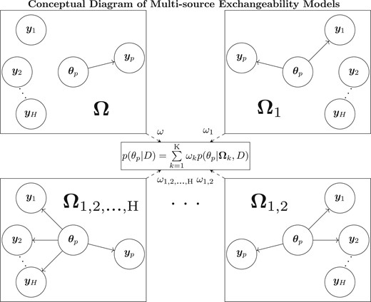
Each MEM is a combination of supplemental sources assumed exchangeable with the primary cohort, in order to estimate the parameters of interest, |$\boldsymbol{\theta}_{p}$|, and is contained within each box for |$\boldsymbol{\Omega}_{k}$|. Within a box the solid arrows |$\boldsymbol{\theta}_{p}$| and the observables, |$\boldsymbol{y}_{h}$|, represent which supplemental sources are assumed exchangeable with the primary cohort within the given MEM. The dashed arrows represent that the posterior model weights for each MEM, |$\omega_{k}$|, are used in calculating the weighted average of each MEM’s posterior distribution, |$p(\theta_{p} | \boldsymbol{\Omega}_{k}, D)$|, to be used for posterior inference, |$p(\theta_{p}|D)$|.
There are two important points to note regarding Theorem 3.1. First, consistency is only attained in the presence of large sample sizes for both the primary and the supplemental cohorts. This property is illustrated in Figure 1 of supplementary material available at Biostatistics online, which presents the model weights as a function of sample size for the case with three supplemental cohorts, where model 2 is the correct model (i.e., |$\mu=\mu_{1}$| and |$\mu \neq \mu_{h}$| for |$h=2,3$|). We see that the model weight converges to 1 when the sample size is large for all cohorts (b) but not when the sample size for the primary cohort is large and the sample size for the supplemental cohorts is constant (a). Second, we illustrate the advantage of specifying the priors on the source-specific inclusion weights, rather than on the model weights, in Figure 1(c) and (d) of supplementary material available at Biostatistics online. These figures present the model weights as a function of sample size for when the prior is specified on the source-specific inclusion weights using |$\pi_{n}$| and when the prior is specified on the model weights in a standard BMA approach using prior weights analogous to |$\pi_{n}$| for the case when there are three supplemental cohorts and model 5 is the correct model (i.e., |$\mu=\mu_{h}$| for |$h=1,2$| and |$\mu\neq\mu_{3}$|). In this case, the model weights are consistent when the prior is specified on the source-inclusion probabilities but not when the prior is specified on the model weights. This is true even when the sample sizes for both the primary and the supplemental cohorts are large, suggesting that the prior specification on the model is not adequate for all situations in our context.
Because bias arising from integrating multisource data is avoided when shrinkage is effectuated using only truly exchangeable sources, consistency is an important property for any multi-source integration approach. The fact that the MEM estimators are consistent for both priors also demonstrates flexibility to accommodate a wide variety of prior beliefs pertaining to source inclusion. As noted in Section 3.1, the posterior mean is a weighted average of the model-specific posterior means, which, in combination with Theorem 3.1, allows us to conclude that the posterior mean will be consistent for the true mean assuming |$\pi_{e}$| and |$\pi_{n}$|.
As |$n, n_{1},\ldots,n_{H} \to \infty$|, |$E\left(\mu\vert D\right) \xrightarrow{a.s} \mu$| with priors |$\pi_{e}$| and |$\pi_{n}$|.
The proof of Corollary 3.2 is a result of the consistency of the sample mean by the strong law of large numbers, Theorem 3.1 and Slutsky’s Theorem.
4. Simulation studies to establish small-sample properties
In this section, we evaluate the small-sample properties of our proposed approach and compare them to two existing methods for integrating supplementary information into the analysis of a primary data set.
4.1. Simulation design
Our simulation study considers scenarios that involve a single primary cohort and three supplemental cohorts: |$S_{1},S_{2},S_{3}$|. We assume that |$n=n_{h}=100$| and |$\sigma=\sigma_{h}=4$| for |$h=1,2,3$| (i.e., that the sample size and standard deviations are equal for all sources of data). This assumption allows us to evaluate performance without having to discern differences attributable to differing sample sizes or sampling-level variances. Four scenarios are evaluated with different assumptions regarding the sample means. The first scenario considers the case where the sample means were equal for all supplemental sources: |$\bar{x}_{1}=\bar{x}_{2}=\bar{x}_{3}=-4$|. The second scenario considers the case where the sample means for the first two sources were identical, but the third was very different:|$\bar{x}_{1}=\bar{x}_{2}=-10, \bar{x}_{3}=2$|. The third scenario represents the case where the sample means were different for all three supplemental sources: |$\bar{x}_{1}=-10,\; \bar{x}_{2}=-4,\; \bar{x}_{3}=2$|. The fourth scenario considers the case where the sample means for the first two supplemental sources were similar, but the third was very different: |$\bar{x}_{1}=-10,\; \bar{x}_{2}=-9.25,\; \bar{x}_{3}=2$|.
For each scenario, we simulate data for the primary cohort with a true |$\mu$| that varied across an equally spaced grid of 420 points from |$-$|15 to 6. Data are analyzed with one of the four approaches for each simulated trial: (1–2) MEMs with |$\pi_{e}$| and |$\pi_{n}$| priors; (3) the empirical Bayes implementation of the commensurate prior approach (CP) (Hobbs and others, 2011); and (4) a standard hierarchical model (SHM) with a uniform hyperprior for the common inter-source standard deviation over the interval (0,50) (Spiegelhalter and others, 2004). Additional values of upper limits for the uniform distribution were explored, but all results performed similarly under the considered scenarios. A total of 10 000 simulated studies are completed for each |$\mu$| for approaches 1 through 3, while 1000 simulated studies are completed at each |$\mu$| for approach 4. The performance of each approach is summarized as a function of |$\mu$| by bias, coverage of the 95% HPD interval, and measures of data integration (as explained in Section 4.2). All calculations are completed with R (R Core Team, 2013).
4.2. Dynamic borrowing
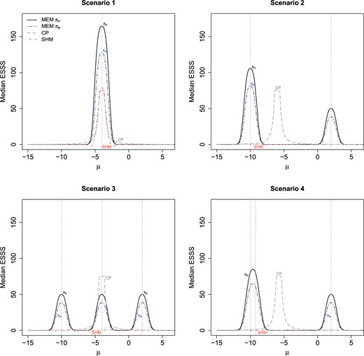
Median effective supplemental sample size using MEM with |$\pi_{e},\pi_{n}$| priors, CP, and SHM under each scenario. Dashed vertical lines are used to represent assumed observed values of the supplemental group means for each scenario.
Figure 2 plots median ESSS curves obtained from our simulation study as a function of |$\mu$|. In Scenario 1, wherein the primary and supplemental data are truly exchangeable, all methods incorporated a substantial amount of supplementary data when the true mean is equal or close to |$-$|4, but the MEM approaches resulted in approximately 1.7 and 2.2 times larger median ESSS (for priors |$\pi_{e}$| and |$\pi_{n}$|, respectively) than CP and SHM when |$\mu=-4$|.
Scenarios 2–4 illustrate that the SHM consistently fails to incorporate supplementary information in the presence of heterogeneity among the supplemental sources. Similar results were observed when using alternative values for the hyperprior upper limit at 5, 10, 20, and 100, as well. The maximum ESSS was larger for |$\pi_{n}$| than |$\pi_{e}$|, in general. In addition, |$\pi_{n}$| resulted in a higher maximum ESSS than CP in 2 of the 3 scenarios, while |$\pi_{e}$| had a higher maximum sample size than CP in 1 of the 3. Moreover, MEMs facilitate flexible patterns of dynamic borrowing, such that ESSS is maximized at the observed supplemental cohort means and minimized in regions devoid of supplemental information. In contrast, CP, which assumes exchangeability among all supplemental sources, yielded high median ESSS in regions without support from the supplemental information. As a result, the two MEM approaches resulted in larger effective regions of borrowing when compared with CP.
4.3. Bias and coverage
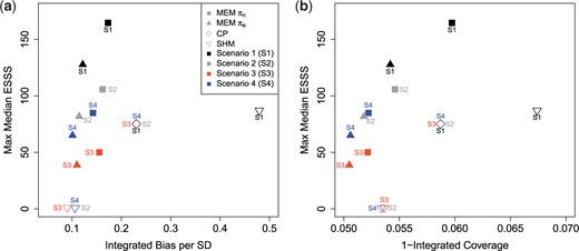
This section evaluates trade-offs between the extent to which one can enhance efficiency through integrating supplementary information (as characterized by ESSS) while maintaining other desirable inferential properties. Figure 3(a) and (b) presents scatter plots that illustrate maximum ESSS as a function of integrated bias per standard deviation (left) and 1-integrated 95% HPD coverage (right). Integrated bias per standard deviation is calculated via Riemann integration of the absolute value of the bias over the simulated points divided by the simulated standard deviation. Integrated coverage is calculated via Riemann integration of the coverage over the simulated points. Additional plots depicting coverage of the 95% HPD interval estimators, bias, and MSE as functions of |$\mu$| can be found in Appendix C of the supplementary material available at Biostatistics online.
Figure 3(a) effectively demonstrates that both CP and SHM intrinsically favor extreme bias versus efficiency trade-offs. This is most evident for the SHM, which either gains efficiency at the expense of a substantial increase in integrated bias (Scenario 1) or exhibits no bias but also no increase in efficiency due to its inability to leverage supplemental information in the presence of heterogeneity in the supplemental cohorts (Scenarios 2–4). In contrast, CP, represented by diamonds, integrated supplemental information in all scenarios but resulted in an identical level of both maximum ESSS and bias for all four scenarios. As a result, the MEM approach resulted in less integrated bias than CP, in all cases, with |$\pi_{e}$| illustrating a 47% to 56% decrease in integrated bias and |$\pi_{n}$| illustrating a 25& to 38% decrease in integrated bias compared with CP. In fact, even in the scenario most favorable to CP and SHM (Scenario 1), MEMs effectuated estimators that attained both less bias and more efficiency.
Similar trends were observed in Figure 3(b), which describes maximum ESSS as a function of 1-integrated coverage. The MEM approach outperforms CP with |$\pi_{e}$| yielding greater coverage in 4 of 4 cases and |$\pi_{n}$| providing greater coverage in 3 of 4 cases, while the SHM exhibits either worse integrated coverage than MEMs (Scenario 1) or adequate coverage with essentially no borrowing (Scenarios 2–4).
Plots demonstrating bias versus shrinkage trade-offs using the methods of CP, SHM, and MEM with |$\pi_{e},\pi_{n}$| source-inclusion priors. Note that CP overlaps for all four scenarios.
5. Application to a regulatory tobacco clinical trial
This section presents a case study illustrating the application of MEMs and competing approaches to data from a recently completed randomized trial of VLNC cigarettes. CENIC-p1 was a randomized trial devised to evaluate the effect of reducing the nicotine content of cigarettes on tobacco use and dependence (Donny and others, 2015). Subjects were randomized equally to one of the seven treatment groups, consisting of a usual brand cigarette condition and six conditions with investigational cigarettes that contained a range of nicotine contents from 15.8 mg of nicotine per gram of tobacco (15.8 mg/g group; approximately the amount of nicotine found in commercially available cigarettes) to VLNC cigarettes with 0.4 mg of nicotine per gram of tobacco (0.4 mg/g group). In addition, one treatment group received cigarettes with 0.4 mg of nicotine per gram of tobacco with high tar to evaluate the impact of tar yield on the effect of VLNC cigarettes (0.4 mg/g, HT group). Our case study compares the change from baseline in cigarettes smoked per day (CPD) between the 0.4 mg/g group and the 15.8 mg/g group.
There are several supplementary sources of data available that could be integrated into our analysis to achieve a more precise estimate of the effect of VLNC cigarettes. First, the usual brand and 0.4 mg/g, HT groups from CENIC would be expected to have similar outcomes to the 15.8 mg/g and 0.4 mg/g groups, respectively, if nicotine is the primary driver of smoking behavior. These data should not be assumed exchangeable, however, due to the impact of “product switching” (i.e., assigning subjects to cigarettes different than their usual brand is likely to impact smoking behavior, regardless of the nicotine content of the new cigarette) and tar yield. In addition, data are also available from two historical trials of VLNC cigarettes (Hatsukami and others, 2010, 2013). We will consider the VLNC cigarette group from Hatsukami and others (2013) and the 0.05 mg nicotine cigarettes group from Hatsukami and others (2010). Both trials used VLNC cigarettes with similar nicotine content to the 0.4 mg/g group from CENIC-p1, but neither trial used an equivalent to the 15.8 mg/g control condition and, therefore, these historical sources will only provide supplemental data for the VLNC condition. We note that the amount of nicotine in a cigarette can be quantified by either the nicotine yield or the nicotine content. CENIC-p1 used the nicotine content, whereas the two historical studies used the nicotine yield, but the nicotine content of the cigarettes was similar. In summary, we have three potential supplemental sources for the 0.4 mg/g group (0.4 mg/g, HT group from CENIC-p1, Hatsukami and others (2013), Hatsukami and others (2010)) and one potential supplemental source for the 15.8 mg/g group (usual brand group from CENIC-p1).
A summary of the observed data describing the mean and standard deviation for the change in CPD for the primary and supplementary data sources can be found in the upper panel of Table 1. Results for the CENIC, 0.4 mg/g group and the CENIC, 0.4 mg/g, HT group are nearly identical, suggesting that exchangeability might be a reasonable assumption for these two cohorts, whereas the data from Hatsukami and others (2013) and Hatsukami and others (2010) were not consistent with the CENIC 0.4 mg/g group. An ideal method would exhibit the flexibility to integrate the data from the 0.4 mg/g, HT group into the primary analysis, while giving little weight to the data from Hatsukami and others (2013) and Hatsukami and others (2010). The two control populations (CENIC 15.8 mg/g and CENIC usual brand) exhibited similar but not entirely consistent results, indicating that some amount of smoothing is appropriate but not to the same extent as for the two 0.4 mg/g conditions.
Summary statistics for change in cigarettes smoked daily since baseline by group and posterior model estimates and ESSS for no borrowing, MEM |$\pi_{e}$|, MEM |$\pi_{n}$|, CP, and SHM
| Study | Source | Mean change | SD | ||
|---|---|---|---|---|---|
| Control groups | CENIC, 15.8 mg/g group (n = 110) | P | 5.90 | 9.15 | |
| CENIC, usual brand group (n = 112) | 1 | 7.33 | 8.38 | ||
| Treatment groups | CENIC, 0.4 mg/g group (n = 109) | P | |$-$|0.23 | 6.79 | |
| CENIC, 0.4 mg/g, HT group (n = 116) | 1 | |$-$|0.15 | 6.71 | ||
| Hatsukami and others (2013) (n = 55) | 2 | |$-$|4.24 | 9.02 | ||
| Hatsukami and others (2010) (n = 32) | 3 | |$-$|7.08 | 7.02 | ||
| Group | Weight | No borrowing | MEM|${\boldsymbol \pi}_{e}$| | MEM|${\boldsymbol \pi}_{n}$| | CP | SHM |
| Control | |$\omega$| | 1.000 | 0.861 | 0.212 | — | — |
| |$\omega_{1}$| | 0.000 | 0.139 | 0.788 | — | — | |
| Treatment | |$\omega$| | 1.000 | 0.691 | 0.423 | — | — |
| |$\omega_{1}$| | 0.000 | 0.305 | 0.566 | — | — | |
| |$\omega_{2}$| | 0.000 | 0.003 | 0.007 | — | — | |
| |$\omega_{3}$| | 0.000 | 0.000 | 0.000 | — | — | |
| |$\omega_{1,2}$| | 0.000 | 0.001 | 0.005 | — | — | |
| |$\omega_{1,3}$| | 0.000 | 0.000 | 0.000 | — | — | |
| |$\omega_{2,3}$| | 0.000 | 0.000 | 0.000 | — | — | |
| |$\omega_{1,2,3}$| | 0.000 | 0.000 | 0.000 | — | — | |
| Control | 5.90 (0.87) | 6.01 (0.89) | 6.52 (0.61) | 6.21 (0.77) | 5.87 (0.85) | |
| Control ESSS | 0.0 | 18.5 | 105.0 | 31.3 | 5.2 | |
| Treatment | |$-$|0.23 (0.65) | |$-$|0.22 (0.55) | |$-$|0.21 (0.47) | |$-$|0.84 (0.53) | |$-$|0.29 (0.65) | |
| Treatment ESSS | 0.0 | 36.5 | 68.2 | 56.8 | 0.7 | |
| |$\Delta$|(Trt|$-$|Con) | |$-$|6.12 (1.09) | |$-$|6.22 (1.05) | |$-$|6.73 (0.77) | |$-$|7.05 (0.93) | |$-$|6.17 (1.07) | |
The lower panel of Table 1 provides results obtained from five competing approaches: a standard model that does not allow borrowing, MEMs with the |$\pi_{e}$| and |$\pi_{n}$| priors, the empirical Bayesian commensurate prior approach, and the SHM. Figure 4 represents the “bias-variance” trade-off from Table 1 using the percent change in mean estimation and the percent reduction in the posterior standard deviation relative to the standard model that does not allow borrowing. Compared to the standard approach, the MEM approach with the |$\pi_{e}$| prior and the SHM show minimal change from the mean estimate at the expense of minor decreases of 4% and 2%, respectively, in the posterior standard deviation. The MEM approach with |$\pi_{n}$| results in only a 10% change in mean estimation when compared with the standard approach while considerably reducing the posterior standard deviation (29%). This is in contrast to the commensurate prior approach which has a larger percent change in mean estimation than MEMs with |$\pi_{n}$|, but borrowed half as much as the MEM with |$\pi_{n}$| prior with a 14% decrease in the posterior standard deviation relative to the standard approach.
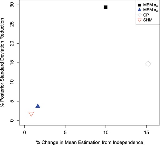
Plot comparing percent change in mean estimation from the standard model with no borrowing and the percent reduction in the posterior standard deviation for the difference between the treatment and control groups in Table 1 for the standard approach with no borrowing to the CP, SHM, and MEM with |$\pi_{e},\pi_{n}$| source-inclusion priors approaches.
6. Discussion
We proposed MEMs, a Bayesian approach for integrating multiple, potentially non-exchangeable, supplemental data sources into the analysis of a primary data source. The modeling strategy was devised to overcome both limitations arising from “single-source” exchangeability models that produce estimators that tend to ignore supplemental data in the presence of heterogeneity and the challenges with implementation of BMA, which is limited by high dimensionality of model prior specification. In contrast, the MEM strategy characterizes source-specific shrinkage parameters that synthesize all possible exchangeability relationships between primary and supplemental cohorts, thereby inducing robustness to heterogeneity. Moreover, the method relies on source-specific prior inclusion probabilities for model specification which, unlike BMA, yield consistent shrinkage estimators. The general approach presented in this manuscript can be adopted in conjunction with any statistically valid likelihood specification and any set of appropriate supplementary cohorts to be considered for potential integration into the primary cohort. The Gaussian case demonstrates how one can influence the shrinkage of supplemental sources through specification of the prior probability of source inclusion, while preserving consistency.
The MEM model formulation reduces the prior space by placing prior weights on the source-inclusion probabilities but other solutions have also been proposed within the BMA framework. Fernández and others (2001) propose 10 “benchmark” priors thath use little or no subjective prior information for specification of the priors on parameters by choice of a single scalar hyperparameter with a corresponding uniform prior for model weights. Eicher and others (2011) explore these benchmark priors in addition to a prior specification corresponding to BIC and identify better performance utilizing the BIC-related prior in situations where there are an extremely large number of models to consider (e.g, |$2^{40}$|) while also noting that the different priors can result in very different posterior results for optimal models. These approaches to prior specification demonstrate that there is a strong relationship between sample size and the number of models that must be averaged over when identifying prior specification that result in optimal performance in finite sample sizes. Eicher and others (2011) also note that different prior specifications on the model weights did not have much impact, but our results suggest that different priors can greatly affect posterior estimation. BMA may also be approximated using the MC|$^{3}$| algorithm for model averaging as proposed by Madigan and others (1995), but this may be infeasible for large |$K$| due to computation considerations as the chain may fail to consider all models. In contrast, relying on source-inclusion prior probabilities, the MEM model formulation addresses these limitations.
A limitation of any method that attempts to utilize supplemental information is that data integration naturally induces bias. We attempt to control bias through a model specification that facilitates source-specific shrinkage parameters, thereby inducing flexibility in the presence of non- or partially exchangeable supplemental cohorts. Our simulation studies and analytical findings demonstrate the extent to which the proposed MEM approach effectively integrates supplemental information while minimizing bias. Averaging over our four scenarios and two priors, MEMs achieved 41% less integrated bias while effectuating a 93% larger maximum effective supplemental sample size when compared with the commensurate prior approach.
The definition of exchangeability used, where |$\mu=\mu_{h}$|, may be seen as unnecessarily stringent. The proposed MEM framework enables source-specific shrinkage to an extent defined by the empirical evidence for exchangeability such that sampling observables arise from identical distributional forms. As an alternative model, the strict assumption of equality could be relaxed by allowing some small term, |$\epsilon_{h}>0$|, potentially specified for each source, such that the extent of shrinkage is determined by |$\mu=\mu_{h}+\epsilon_{h}$|. This model, however, would not be identifiable without inducing sparsity on the domain of |$\epsilon_{h}$|, perhaps with a spike-and-slab prior. This would require additional hyperparameter specification beyond that of the MEM framework, which would complicate the calibration to control frequentist error in practical application.
Another limitation is that the type of study, retrospective/observational versus prospective/randomized, affects the quality and reliability of the resulting estimates, and therefore consideration of design type should be taken into account. For example, as conveyed in Pocock’s “Acceptability Criteria,” (1976), decisions pertaining to which supplemental sources should be considered for integrative analysis should be based on the study objectives as well as controlling sources of potential bias arising from inconsistent eligibility criteria, application of the interventions, or outcome ascertainment. Similarly, when using data arising from non-randomized designs, confounding due to selection bias needs to be accounted for in some manner, such as through existing methods for causal inference using propensity scoring, inverse-probability weighting, or matching. We endeavor to extend the methodology to facilitate integration of multiple trials while accounting for confounding from non-randomized designs as future work.
7. Software
The R code for the simulation and data illustration is available for download at https://github.com/JSKoopmeiners/Multi-Source-Exchangeability-Models.
Supplementary Material
Supplementary material is available online at http://biostatistics.oxfordjournals.org.
Acknowledgements
We would like to thank our collaborators, Drs Eric Donny and Dorothy Hatsukami, for providing the data used in Section 5. Conflict of Interest: None declared.
Funding
National Institutes of Health (NIH) grant (P30-CA016672) from the National Cancer Institute and NIH grants (U54-DA031659 and R03-DA041870) from the National Institute on Drug Abuse and FDA Center for Tobacco Products (CTP). The content is solely the responsibility of the authors and does not necessarily represent the official views of the NIH or FDA CTP.
