


ABSTRACT
Motivated by the need for computationally tractable spatial methods in neuroimaging studies, we develop a distributed and integrated framework for estimation and inference of Gaussian process model parameters with ultra-high-dimensional likelihoods. We propose a shift in viewpoint from whole to local data perspectives that is rooted in distributed model building and integrated estimation and inference. The framework’s backbone is a computationally and statistically efficient integration procedure that simultaneously incorporates dependence within and between spatial resolutions in a recursively partitioned spatial domain. Statistical and computational properties of our distributed approach are investigated theoretically and in simulations. The proposed approach is used to extract new insights into autism spectrum disorder from the autism brain imaging data exchange.
1 INTRODUCTION
The proposed methods are motivated by the investigation of differences in brain functional organization between people with autism spectrum disorder (ASD) and their typically developing peers. The autism brain imaging data exchange (ABIDE) neuroimaging study of resting-state functional magnetic resonance imaging (rfMRI) aggregated and publicly shared neuroimaging data on participants with ASD and neurotypical controls from 16 international imaging sites. Relationships between activated brain regions of interest (ROIs) during rest can be characterized by functional connectivity between ROIs using rfMRI data. Functional connectivity between 2 ROIs is typically estimated from the subject-specific correlation constructed from the rfMRI time series (Shehzad et al., 2014). To avoid the computational burden of storing and modeling a large connectivity matrix, the rfMRI time series is averaged across voxels in each ROI before computing the cross-ROI correlation and modeling its relationship with covariates. Other approaches for quantifying covariate effects on correlation are primarily univariate (see, eg, Shehzad et al., 2014). These standard approaches are substantially underpowered to detect small effect sizes and obscure important variation within ROIs. While ABIDE data have led to some evidence that ASD can be broadly characterized as a brain dysconnection syndrome, findings have varied across studies (Alaerts et al., 2014; Di Martino et al., 2014). Computationally and statistically efficient estimation of functional connectivity maps is essential in identifying ASD dysconnections. In this paper, we show how to estimate the effect of covariates, including ASD, on over 6.5 million within- and between-ROI correlations in approximately 4 hours using 4 GB of RAM. In contrast, a conventional analysis takes over 190 hours and 175 GB of RAM.
The first component of our efficient approach is to leverage the spatial dependence within and between all voxels in ROIs using Gaussian process models (Banerjee et al., 2014; Cressie, 1993; Cressie and Wikle, 2015). Denote the rfMRI outcomes |$\lbrace y_i(\boldsymbol{s})\rbrace _{i=1}^N$| for N independent samples at one of S voxels |$\boldsymbol{s}\in \mathcal {S}$|. The joint distribution of |$y_i(\mathcal {S})$| is assumed multivariate Gaussian and known up to a vector of parameters of interest |$\boldsymbol{\theta }$|. Without further modeling assumptions or dimension reduction techniques, maximum likelihood estimation has memory and computational complexity of |$O(NS^2)$| and |$O(NS^3)$|, respectively, due to the S-dimensional covariance matrix. For inference on |$\boldsymbol{\theta }$| when S is large, the crux of the problem is to adequately model the spatial dependence without storing or inverting a large covariance matrix.
This problem has received considerable attention (Bradley et al., 2016; Heaton et al., 2019; Liu et al., 2020; Sun et al., 2011). Solutions include, for example, the composite likelihood (CL) (Lindsay, 1988), the nearest-neighbor Gaussian process (NNGP) (Datta et al., 2016; Finley et al., 2019), spectral methods (Fuentes, 2007), tapered covariance functions (Furrer et al., 2006; Kaufman et al., 2008; Stein, 2013), low-rank approximations (Cressie and Johannesson, 2008; Nychka et al., 2015; Zimmerman, 1989), and combinations thereof (Sang and Huang, 2012). Stein (2013) details shortcomings of the aforementioned methods, which are primarily related to loss of statistical efficiency due to simplification of the covariance matrix or its inverse. Moreover, these methods remain computationally burdensome when S is very large, a problem that is further exacerbated when the covariance structure is nonstationary.
We propose a new distributed and integrated framework for big spatial data analysis. We consider a recursive partition of the spatial domain |$\mathcal {S}$| into M nested resolutions with disjoint sets of spatial observations at each resolution, and build local, fully specified distributed models in each set at the highest spatial resolution. The main technical difficulty arises from integrating inference from these distributed models over 2 levels of dependence: between sets in each resolution and between resolutions. The main contribution of this paper is a recursive estimator that integrates inference over all sets and resolutions by alternating between levels of dependence at each integration step. We also propose a sequential integrated estimator that is asymptotically equivalent to the recursive integrated estimator but reduces the computational burden of recursively integrating over multiple resolutions. The resulting multiresolution recursive integration (MRRI) framework is flexible, statistically efficient, and computationally scalable through its formulation in the MapReduce paradigm.
The rest of this paper is organized as follows. Section 2 establishes the formal problem setup, and describes the distributed model-building step and the recursive integration scheme for the proposed MRRI framework. Section 3 evaluates the proposed frameworks with simulations. Section 4 presents the analysis of data from ABIDE. Proofs, additional results, ABIDE information, and an R package are provided as supplementary materials.
2 RECURSIVE MODEL INTEGRATION FRAMEWORK
2.1 Problem set-up
Suppose we observe |$y_i(\boldsymbol{s})=\alpha _i(\boldsymbol{s}) + \epsilon _i(\boldsymbol{s})$| the ith observation at location |$\boldsymbol{s}\in \mathbb {R}^d$|, |$i=1, \ldots , N$| independently and |$\boldsymbol{s}\in \mathcal {S}$| a set of S locations, where |$\alpha _i(\cdot )$| characterizes the spatial variations and |$\epsilon _i(\cdot )$| is an independent normally distributed measurement error with mean 0 and variance |$\sigma ^2$| independent of |$\alpha _i(\cdot )$|. The nugget variance |$\sigma ^2$| is assumed fixed across i and |$\boldsymbol{s}$|. We justify this assumption for our neuroimaging application below, and discuss extensions in Section 5. Suppose for each replicate i we observe q explanatory variables |$\boldsymbol{X}_i(\boldsymbol{s}) \in \mathbb {R}^q$|. We denote by |$\mathcal {S}=\lbrace \boldsymbol{s}_j\rbrace _{j=1}^S$| the set of locations and define |$y_i(\mathcal {S})=\lbrace y_i(\boldsymbol{s}_j)\rbrace _{j=1}^S$| and |$\boldsymbol{X}_i(\mathcal {S})=\lbrace \boldsymbol{X}_i(\boldsymbol{s}_j)\rbrace _{j=1}^S$|.
In Section 4, |$\mathcal {S}$| is the set of voxels in the left and right precentral gyri, visualized in the supplement, and |$d=3$|. Outcomes |$\lbrace y_i(\boldsymbol{s})\rbrace _{i=1}^N$| consist of the thinned rfMRI time series at voxel |$\boldsymbol{s}$| for ABIDE participants passing quality control, where the thinning removes every second time point to remove autocorrelation; autocorrelation plots are provided as supplementary materials. Thinning avoids the bias occasionally introduced by other approaches (Monti, 2011) and aligns with usual rfMRI autocorrelation assumptions (Arbabshirani et al., 2014). Specifically, for participant |$n\in \lbrace 1, \ldots , 774\rbrace$| and voxel |$\boldsymbol{s}\in \mathcal {S}$| with a time series of length |$2T_n$|, the outcome |$y_i(\boldsymbol{s})$| consists of the (centered and standardized) rfMRI outcome at time point |$t \in \lbrace 2,4, \ldots , 2T_n\rbrace$|, where |$i= t + \sum _{n^\prime \lt n} T_{n^\prime }$| indexes the participants and time points. This thinning results in |$N=75888$| observations of |$y_i(\boldsymbol{s})$|. While we focus on 2 ROIs for simplicity of exposition, our approach generalizes to multiple ROIs. Variables |$\boldsymbol{X}_i(\boldsymbol{s})=\boldsymbol{X}_i$| consist of an intercept, ASD status, age, sex, and the age by ASD status interaction.
We assume that |$\alpha _i(\cdot )$| is a Gaussian process with mean function |$\mu \lbrace \cdot ; \boldsymbol{X}_i(\cdot ), \boldsymbol{\beta }\rbrace$| and positive-definite covariance function |$C_{\alpha }\lbrace \cdot ,\cdot ; \boldsymbol{X}_i(\cdot ), \boldsymbol{\gamma }\rbrace$|. We further assume that |$\mu \lbrace \mathcal {S}; \boldsymbol{X}_i(\mathcal {S}), \boldsymbol{\beta }\rbrace$| is known up to a parameter |$\boldsymbol{\beta }\in \mathbb {R}^{q_1}$|, and |$C_{\alpha }\lbrace \mathcal {S}, \mathcal {S}; \boldsymbol{X}_i(\mathcal {S}), \boldsymbol{\gamma }\rbrace$| is known up to a parameter |$\boldsymbol{\gamma }\in \mathbb {R}^{q_2}$|: |$C_{\alpha }\lbrace \boldsymbol{s}_1, \boldsymbol{s}_2; \boldsymbol{X}_i(\boldsymbol{s}_1), \boldsymbol{X}_i(\boldsymbol{s}_2), \boldsymbol{\gamma }\rbrace =\mbox{Cov}\lbrace \alpha _i(\boldsymbol{s}_1), \alpha _i(\boldsymbol{s}_2) \rbrace$|. The distribution of |$y_i(\mathcal {S})$| is S-variate Gaussian with mean |$\mu \lbrace \mathcal {S}; \boldsymbol{X}_i(\mathcal {S}), \boldsymbol{\beta }\rbrace$| and covariance |$\boldsymbol{C}\lbrace \mathcal {S}, \mathcal {S}; \boldsymbol{X}_i(\mathcal {S}), \boldsymbol{\gamma }, \sigma ^2\rbrace =[C_{\alpha }\lbrace \boldsymbol{s}_r, \boldsymbol{s}_t; \boldsymbol{X}_i(\boldsymbol{s}_r), \boldsymbol{X}_i(\boldsymbol{s}_t), \boldsymbol{\gamma }\rbrace ]_{r,t=1}^{S,S} + \sigma ^2 \boldsymbol{I}_S$|. We define |$\boldsymbol{\theta }=(\boldsymbol{\beta }, \boldsymbol{\gamma }, \sigma ^2) \in \mathbb {R}^p$| the parameter of interest, |$p=q_1+q_2+1$|. The standardization of the rfMRI time series justifies our assumption of a homogeneous |$\sigma ^2$| across i and |$\boldsymbol{s}$|. We allow the covariance to depend on |$\boldsymbol{X}_i(\mathcal {S})$| and to exhibit some nonstationarity. In Section 4, |$C_{\alpha }$| borrows from Paciorek and Schervish (2003) and takes the form
where |$r_{ij}=\exp \lbrace \boldsymbol{X}_i^\top \boldsymbol{\rho }(\boldsymbol{s}_j)\rbrace$| models the effect of |$\boldsymbol{X}_i$| on the correlation between voxels through |$\boldsymbol{\rho }(\boldsymbol{s}_j) \in \mathbb {R}^q$|. Both |$\boldsymbol{\rho }(\boldsymbol{s}_j)$| and |$\tau (\boldsymbol{s}_j, \boldsymbol{s}_{j^\prime })$| are specified in Section 4.
2.2 A Shift from Whole to Local Data Perspectives
We propose a recursive partition of |$\mathcal {S}$| into multiple resolutions, with multiple sets at each resolution. Let |$\otimes 2$| denote the outer product of a vector with itself, namely |$\boldsymbol{a}^{\otimes 2}=\boldsymbol{a}\boldsymbol{a}^\top$|. Using the notation of Katzfuss (2017), denote |$\mathcal {A}_0=\mathcal {S}$| and partition |$\mathcal {S}$| into |$K_1$| (disjoint) regions |$\lbrace \mathcal {A}_1, \ldots , \mathcal {A}_{K_1}\rbrace$| that are again partitioned into |$K_2$| (disjoint) subregions |$\lbrace \mathcal {A}_{k_11}, \ldots , \mathcal {A}_{k_1K_2}\rbrace _{k_1=1}^{K_1}$|, and so on up to level M, that is,|$\mathcal {A}_{k_1 \ldots k_{m-1}}=\cup _{k_m=1, \ldots , K_m} \mathcal {A}_{k_1 \ldots k_{m-1} k_m}$|, |$k_{m-1} \in \lbrace 1, \ldots , K_{m-1}\rbrace$|, |$m=1, \ldots , M$|, where |$K_0=1$|. For completeness, let |$k_0=0$|. An example of a recursive partition of observations on a 2-dimensional spatial domain for |$M=2$| resolutions is provided as supplementary materials. For resolution |$m \in \lbrace 1, \ldots , M\rbrace$|, denote |$S_{k_1\ldots k_m}$| the size of |$\mathcal {A}_{k_1\ldots k_m}$|, with |$S_0=S$|. Further define |$k_{\max }=\max k_m$| with the maximum taken over |$k_m=1, \ldots , K_m$| and |$m=1, \ldots , M$|. Due to that fact that |$S_0=\sum _{m=1}^M \sum _{k_m=1}^{K_m} S_{k_1\ldots k_M}$|, |$S_{k_1\ldots k_M}, K_m \lt S_0$|. We further recommend that values of M and |$K_m$| be chosen so that |$S_{k_1\ldots k_M}$| and |$K_m, m=1, \ldots , M$| are relatively small compared to |$S_0$|, and we generally recommend |$S_{k_1\ldots k_M} \ge 25$|.
This idea appears similar to MRA models (Katzfuss, 2017; Katzfuss and Gong, 2020; Nychka et al., 2015). Where they integrate from global to local levels, however, we build local models at the highest resolution and recursively integrate inference from the highest to the lowest resolution. Unlike MRA models, we also incorporate unstructured dependence within all spatial resolutions using the generalized method of moments (GMM) (Hansen, 1982) framework, described in Section 2.3.
At resolution M for |$k_M \in \lbrace 1, \ldots , K_M \rbrace$|, the likelihood of the data in set |$\mathcal {A}_{k_1 \ldots k_M}$| is given by |$y_i(\mathcal {A}_{k_1\ldots k_M}) \sim \mathcal {N}[\mu \lbrace \mathcal {A}_{k_1\ldots k_M}; \boldsymbol{X}_i(\mathcal {A}_{k_1\ldots k_M}), \boldsymbol{\beta }\rbrace ; \boldsymbol{C}\lbrace \mathcal {A}_{k_1\ldots k_M}, \mathcal {A}_{k_1\ldots k_M}; \boldsymbol{X}_i(\mathcal {A}_{k_1\ldots k_M}), \\\boldsymbol{\gamma }, \sigma ^2\rbrace ]$|. We model the mean of the spatial process through |$\mu \lbrace \mathcal {A}_{k_1\ldots k_M}; \boldsymbol{X}_i(\mathcal {A}_{k_1\ldots k_M}), \boldsymbol{\beta }\rbrace =h \lbrace \boldsymbol{X}^\top _i(\mathcal {A}_{k_1\ldots k_M}) \boldsymbol{\beta }\rbrace$|. The function h is assumed known and will most often be the linear function |$h\lbrace \boldsymbol{X}^\top _i(\mathcal {A}_{k_1\ldots k_M}) \boldsymbol{\beta }\rbrace = \boldsymbol{X}^\top _i(\mathcal {A}_{k_1\ldots k_M}) \boldsymbol{\beta }$|. In Section 3, we investigate the performance of our method when h is the linear and log functions. In Section 4, |$\mu \lbrace \boldsymbol{s}_j; \boldsymbol{X}_i(\boldsymbol{s}_j), \boldsymbol{\beta }\rbrace =\beta$| for |$\boldsymbol{s}_j \in \mathcal {A}_{k_1\ldots k_M}$| due the centering of each time series, and |$\boldsymbol{C}$| is the nonstationary covariance function in (1). Due to the recursive partitioning, |$S_{k_1\ldots k_M}$| is small and the likelihood tractable. Denote the log-likelihood in |$\mathcal {A}_{k_1\ldots k_M}$| as |$\ell _{k_1\ldots k_M}(\boldsymbol{\theta })$| and the score function as |$\boldsymbol{\Psi }_{k_1\ldots k_M}(\boldsymbol{\theta })=\nabla _{\boldsymbol{\theta }} \ell _{k_1\ldots k_M}(\boldsymbol{\theta })=\sum _{i=1}^N \boldsymbol{\psi }_{i,k_1\ldots k_M}(\boldsymbol{\theta })$|. The maximum likelihood estimator (MLE) |$\widehat{\boldsymbol{\theta }}_{k_1\ldots k_M}$| of |$\boldsymbol{\theta }$| in |$\mathcal {A}_{k_1\ldots k_M}$| is obtained by maximizing the log-likelihood, or equivalently solving |$\boldsymbol{\Psi }_{k_1\ldots k_M}(\boldsymbol{\theta })=\boldsymbol{0}$|.
The literature is replete with methods for choosing partitions; see Heaton et al. (2019) for an excellent review. The covariance model need only be specified within each block at the highest resolution. We thus recommend that practitioners recursively partition the domain such that the covariance model within each block at the highest resolution can be easily specified, consistently and tractably estimated, and homogeneous across blocks in the sense that the outcome within each block is generated from the same model. In Section 4, we recursively partition voxels in the left and right precentral gyri separately into |$K_1=2$|, |$K_2=K_3=4$| disjoint sets based on nearest neighbors, |$M=3$|; the sets |$\mathcal {A}_{k_1\ldots k_m}$| consist of the union of the disjoint partition sets in the 2 gyri at each resolution |$m \in \lbrace 1, \ldots , M\rbrace$|. This strategy ensures that each |$\mathcal {A}_{k_1\ldots k_M}$| contains locations from both gyri, so that gyri-specific parameters are identifiable in all sets |$\mathcal {A}_{k_1\ldots k_M}$|, |$k_M=1\ldots , K_M$|. As another example, a practitioner may choose to partition their domain such that the outcome in each block at the highest resolution has a simple local covariance structure, such as a Gaussian or exponential covariance function (see Section 3 for examples); if only the mean is of interest, with the covariance treated as a nuisance, then a partition with independent observations within each block at the highest resolution would be practical as the model is easy to specify and estimate, and the dependence between blocks is accounted for in the combination steps. The assumption is then that the local covariance structure within all blocks at the highest resolution is the same (extensions are discussed in Section 5). The unstructured covariance between these blocks is captured by the GMM, discussed next.
2.3 Recursive Model Integration
2.3.1 GMM Approach
We now wish to recursively integrate the local models at each resolution. For |$m=M, \ldots , 0$|, let |$k_m \in \lbrace 1, \ldots , K_m\rbrace$| denote the index for the sets at resolution m. We describe a recursive GMM approach that re-estimates |$\boldsymbol{\theta }$| at each resolution |$M-1$| based on an optimally weighted form of the GMM equation from the higher resolution M. At resolution |$M-1$|, we define |$K_{M-1}$| estimating functions based on the score functions from resolution M: for |$k_{M-1}=1, \ldots , K_{M-1}$|,
both in |$\mathbb {R}^{pK_M}$|. The function |$\boldsymbol{\Psi }_{k_1\ldots k_{M-1}}(\boldsymbol{\theta })$| overidentifies |$\boldsymbol{\theta }\in \mathbb {R}^p$|, that is, there are several estimating functions for each parameter. Following Hansen’s (1982) GMM, we propose to minimize the quadratic form |$Q_{k_1\ldots k_{M-1}}(\boldsymbol{\theta })=\boldsymbol{\Psi }^\top _{k_1\ldots k_{M-1}}(\boldsymbol{\theta }) \boldsymbol{W}\boldsymbol{\Psi }_{k_1\ldots k_{M-1}}(\boldsymbol{\theta })$|, with a positive semi-definite weight matrix |$\boldsymbol{W}$|. Hansen (1982) showed that the optimal choice of |$\boldsymbol{W}$| is the inverse of the covariance of |$\boldsymbol{\Psi }_{k_1\ldots k_{M-1}}(\boldsymbol{\theta })$|, which can be consistently estimated by
the variability matrix, and |$\boldsymbol{\psi }_{i,k_1\ldots k_{M-1}}(\widehat{\boldsymbol{\theta }}_{k_1\ldots k_M})=\lbrace \boldsymbol{\psi }_{i,k_1\ldots k_M}(\widehat{\boldsymbol{\theta }}_{k_1\ldots k_{M-1} k_M}) \rbrace _{k_M=1}^{K_M}$|. The matrix |$N^{-1}\boldsymbol{V}_{k_1\ldots k_{M-1}}(\widehat{\boldsymbol{\theta }}_{k_1\ldots k_M})$| estimates dependence between score functions from all sets in |$\mathcal {A}_{k_1\ldots k_{M-1}}$| and thus captures dependence between sets |$\lbrace \mathcal {A}_{k_1\ldots k_M} \rbrace _{k_M=1}^{K_M}$|. This choice is “Hansen” optimal in the sense that, for all possible choices of |$\boldsymbol{W}$|,
has minimum variance among estimators |$\arg \min _{\boldsymbol{\theta }} Q_{k_1\ldots k_{M-1}}(\boldsymbol{\theta })$|. The computation of |$Q^{*}_{k_1\ldots k_{M-1}}(\boldsymbol{\theta })$| in (3) requires inversion of the |$(pK_M)\times (pK_M)$| dimensional matrix |$\boldsymbol{V}^{-1}_{k_1\ldots k_{M-1}}(\widehat{\boldsymbol{\theta }}_{k_1\ldots k_M})$|, substantially smaller than inverting the |$S_{k_1\ldots k_{M-1}}\times S_{k_1\ldots k_{M-1}}$| dimensional matrix in the direct evaluation of the likelihood on set |$\mathcal {A}_{k_1\ldots k_{M-1}}$|. This yields a faster computation than a full likelihood approach on |$\mathcal {A}_{k_1\ldots k_{M-1}}$|. The iterative minimization in (3), however, can be time-consuming because it requires computation of the score functions |$\boldsymbol{\Psi }_{k_1\ldots k_M}$| at each iteration.
In the spirit of Hector and Song (2021), a closed-form meta-estimator asymptotically equivalent to |$\widehat{\boldsymbol{\theta }}_{GMM}$| in (3) that is more computationally attractive is given by
where |$\boldsymbol{S}_{k_1\ldots k_{M-1}}(\widehat{\boldsymbol{\theta }})=-\lbrace \nabla _{\boldsymbol{\theta }} \boldsymbol{\Psi }_{k_1\ldots k_{M-1}}(\boldsymbol{\theta }) \vert _{\boldsymbol{\theta }=\widehat{\boldsymbol{\theta }}} \rbrace ^\top \in \mathbb {R}^{p\times pK_M}$|, and
with |$\boldsymbol{S}_{k_1\ldots k_M}(\widehat{\boldsymbol{\theta }}) = \lbrace \nabla _{\boldsymbol{\theta }} \boldsymbol{\Psi }_{k_1\ldots k_M}(\boldsymbol{\theta }) \vert _{\boldsymbol{\theta }=\widehat{\boldsymbol{\theta }}} \rbrace ^\top \in \mathbb {R}^{p\times p}$|. The sensitivity matrix |$\boldsymbol{S}_{k_1\ldots k_{M-1}}(\widehat{\boldsymbol{\theta }}_{k_1\ldots k_M})$| can be efficiently computed by Bartlett’s identity.
When updating to the next resolution |$M-2$|, it is tempting to proceed again through the GMM approach and to stack estimating functions |$\lbrace \boldsymbol{\Psi }_{k_1 \ldots k_{M-1}} (\boldsymbol{\theta }) \rbrace _{k_{M-1}=1}^{K_{M-1}}$|. This would, however, result in a vector of overidentified estimating functions on |$\boldsymbol{\theta }$| of dimension |$pK_{M-1}K_M$|, and therefore inversion of a |$(pK_{M-1}K_M)\times (pK_{M-1}K_M)$| dimensional covariance matrix. Recursively proceeding this way would lead to the inversion of a large |$(pK_1\ldots K_M)\times (pK_1\ldots K_M)$| dimensional matrix at resolution |$m=0$|, negating the gain in computation afforded by the partition. To avoid this difficulty, we propose weights in the spirit of optimal estimating function theory (Heyde, 1997). These optimally weight GMM estimating functions and reduce their dimension for computationally tractable recursive integration of dependent models.
2.3.2 Weighted OverIdentified Estimating Functions
We define new estimating functions at resolution |$m=M-2$| that optimally weight the estimating functions from resolution |$M-1$|. Let
where |$\boldsymbol{S}^\top _{k_1\ldots k_{M-1}}(\widehat{\boldsymbol{\theta }}_{k_1\ldots k_{M-1}})$| and |$\boldsymbol{V}_{k_1\ldots k_{M-1}}(\widehat{\boldsymbol{\theta }}_{k_1\ldots k_{M-1}})$| are recomputed so as to evaluate the sensitivity and variability at the estimator from resolution |$M-1$|. This formulation can also be viewed as the optimal projection of the estimating function |$\boldsymbol{\Psi }_{k_1\ldots k_{M-1}}(\boldsymbol{\theta })$| onto the parameter space of |$\boldsymbol{\theta }$| (Heyde, 1997). Stacking |$\lbrace \widetilde{\boldsymbol{\Psi }}_{k_1\ldots k_{M-1}}(\boldsymbol{\theta })\rbrace _{k_{M-1}=1}^{K_{M-1}}$| yields |$\boldsymbol{\Psi }_{k_1\ldots k_{M-2}}(\boldsymbol{\theta })$|, a |$pK_{M-1}$| dimensional vector of overidentifying estimating functions on |$\boldsymbol{\theta }$|. Defining |$\boldsymbol{V}_{k_1\ldots k_{M-2}}(\widehat{\boldsymbol{\theta }}_{k_1\ldots k_{M-1}})$| the sample covariance of |$\boldsymbol{\Psi }_{k_1\ldots k_{M-2}}(\boldsymbol{\theta })$| evaluated at |$\widehat{\boldsymbol{\theta }}_{k_1\ldots k_{M-1}}$|, one can again define the closed-form meta-estimator |$\widehat{\boldsymbol{\theta }}_{k_1\ldots k_{M-2}}$| in the fashion of (4). This requires inversion of a |$(pK_{M-1})\times (pK_{M-1})$|-dimensional matrix, substantially smaller than inverting the |$S_{k_1\ldots k_{M-2}}\times S_{k_1\ldots k_{M-2}}$|-dimensional matrix in the full likelihood on set |$\mathcal {A}_{k_1\ldots k_{M-2}}$|.
2.3.3 Recursive Integration Procedure
The recursive integration procedure updates through Sections 2.3.1 and 2.3.2: for each |$k_m=1\ldots , K_m$|, |$m=M-2, \ldots , 1$|, do steps 1 and 2, described next. In step 1, recursively compute |$\boldsymbol{V}_{k_1\ldots k_m}(\widehat{\boldsymbol{\theta }}_{k_1\ldots k_{m+1}})$| and |$\boldsymbol{S}_{k_1\ldots k_m}(\widehat{\boldsymbol{\theta }}_{k_1\ldots k_{m+1}})$| as follows: (i) compute |$\boldsymbol{\psi }_{i,k_1\ldots k_M}(\widehat{\boldsymbol{\theta }}_{k_1\ldots k_{m+1}})$| and obtain |$\boldsymbol{S}_{k_1\ldots k_M}(\widehat{\boldsymbol{\theta }}_{k_1\ldots k_{m+1}})$|; (ii) define |$\boldsymbol{\psi }_{i,k_1\ldots k_{M-1}}(\widehat{\boldsymbol{\theta }}_{k_1\ldots k_{m+1}})=\lbrace \boldsymbol{\psi }_{i,k_1\ldots k_M}(\widehat{\boldsymbol{\theta }}_{k_1\ldots k_{m+1}})\rbrace _{k_M=1}^{K_M}$| and obtain |$\boldsymbol{V}_{k_1\ldots k_{M-1}} (\widehat{\boldsymbol{\theta }}_{k_1\ldots k_{m+1}})$| and |$\boldsymbol{S}_{k_1\ldots k_{M-1}}(\widehat{\boldsymbol{\theta }}_{k_1\ldots k_{m+1}})$|; (iii) obtain |$\widetilde{\boldsymbol{\psi }}_{i,k_1\ldots k_{M-1}}(\widehat{\boldsymbol{\theta }}_{k_1\ldots k_{m+1}})=- \boldsymbol{S}_{k_1\ldots k_{M-1}}\,(\widehat{\boldsymbol{\theta }}_{k_1\ldots k_{m+1}})\, \boldsymbol{V}^{-1}_{k_1\ldots k_{M-1}}\,(\widehat{\boldsymbol{\theta }}_{k_1\ldots k_{m+1}}) \boldsymbol{\psi }_{i,k_1\ldots k_{M-1}}\,(\widehat{\boldsymbol{\theta }}_{k_1\ldots k_{m+1}})$|; and (iv) for |$k_j=k_{M-2}, \ldots , k_m$|, compute
In step 2, compute
where |$\boldsymbol{T}_{k_1\ldots k_m}(\widehat{\boldsymbol{\theta }}_{k_1\ldots k_{m+1}}) =[\lbrace \boldsymbol{S}^\top _{k_1\ldots k_m}(\widehat{\boldsymbol{\theta }}_{k_1\ldots k_{m+1}}) \rbrace _{j} \widehat{\boldsymbol{\theta }}_{k_1\ldots k_m j}]_{j=1}^{K_{m+1}} \in \mathbb {R}^{pK_{m+1}\times p}$| and
At resolution |$m=0$|, we obtain |$\boldsymbol{\psi }_{i,0}(\widehat{\boldsymbol{\theta }}_{k_1}) = \lbrace \widetilde{\boldsymbol{\psi }}_{i,k_1}(\widehat{\boldsymbol{\theta }}_{k_1})\rbrace _{k_1=1}^{K_1} \in \mathbb {R}^{pK_1}$|, |$\boldsymbol{\Psi }_0(\widehat{\boldsymbol{\theta }}_{k_1}) = \lbrace \widetilde{\boldsymbol{\Psi }}_{k_1}(\widehat{\boldsymbol{\theta }}_{k_1}) \rbrace _{k_1=1}^{K_1} \in \mathbb {R}^{pK_1}$| and a final integrated estimator
where
and
can be computed following the recursive procedure.
A toy example illustrating the procedure is given in the supplement. One evaluation at resolution M has computation and memory complexities of |$O(NS_{k_1\ldots k_M}^3)$| and |$O(NS_{k_1\ldots k_M}^2)$| respectively. This evaluation is repeated M times across the recursive integration procedure. The recursive loop inverts each |$(pK_m)\times (pK_m)$| covariance matrix |$O(M)$| times, adding computation and memory complexities |$O\lbrace M(pK_m)^3 \rbrace$| and |$O\lbrace M(pK_m)^2 \rbrace$|, respectively. At each resolution m, inversions and the computation of the |$K_m$| estimators |$\widehat{\boldsymbol{\theta }}_{k_1\ldots k_m}$| can be done in parallel across |$K_m$| computing nodes to further reduce computational costs. This yields computation and memory complexities, respectively, of
Finally, the computation of |$\widehat{\boldsymbol{\theta }}_{k_1\ldots k_m}$| requires no iterative minimization of an objective function, substantially reducing computational costs. The procedure can be fully run on a distributed system, meaning that at no point do the data need to be loaded on a central server or the full |$S\times S$| covariance matrix stored.
While the number of locations |$S_{k_1\ldots k_M}$| in blocks at the highest resolution drives the computational complexity at the distributed step, the number of blocks |$K_m$| at each resolution drives the computational complexity at the combination step through |$k_{\max }$|. Several values of |$K_m$| and M may achieve similar values of |$S_{k_1\ldots k_M}$|, and so a practical consideration concerns the choice of these values. First, we recommend choosing |$K_j$| close to divisors of S so as to achieve a similar number of locations in each block. Next, we recommend choosing values such that neither |$K_j$| nor M is excessively large or small. For example, the toy example in the supplement partitions a |$10\times 10$| grid of locations using |$K_1=K_2=2$|, |$M=2$|. Finally, we show in Section 3 that different choices of M and |$K_m$| lead to similar performances.
2.4 Multiresolution Estimating Function Theory
Let |$\Theta$| the parameter space of |$\boldsymbol{\theta }$|, and denote by |$\boldsymbol{\theta }_0$| the true value of |$\boldsymbol{\theta }$|, defined formally by assumptions as supplementary materials. In this section, we study the asymptotic properties of |$\widehat{\boldsymbol{\theta }}_r$| by formalizing a multiresolution estimating function theory. To do this, define population versions of the estimating functions, their variability, and their sensitivity: for |$k_m=1, \ldots , K_m$|, |$\boldsymbol{\phi }_{i,k_1\ldots k_m}(\boldsymbol{\theta })=\boldsymbol{\psi }_{i,k_1\ldots k_m}(\boldsymbol{\theta })$| for |$m=M,M-1$|, and
where, for |$m=1, \ldots , M$|, |$\boldsymbol{v}_{k_1\ldots k_m}(\boldsymbol{\theta }) = \mathbb {V}_{\boldsymbol{\theta }_0} \left\lbrace \boldsymbol{\phi }_{i,k_1\ldots k_m}(\boldsymbol{\theta }) \right\rbrace$|, |$\boldsymbol{s}^\top _{k_1\ldots k_m}(\boldsymbol{\theta }) = - \mathbb {E}_{\boldsymbol{\theta }_0} \lbrace \nabla _{\boldsymbol{\theta }} \boldsymbol{\phi }_{i,k_1\ldots , k_m}(\boldsymbol{\theta }) \rbrace$|, and |$\boldsymbol{j}_{k_1\ldots k_m}(\boldsymbol{\theta })=\boldsymbol{s}_{k_1\ldots k_m}(\boldsymbol{\theta })\boldsymbol{v}^{-1}_{k_1\ldots k_m}(\boldsymbol{\theta }) \boldsymbol{s}^\top _{k_1\ldots k_m}(\boldsymbol{\theta })$| are the variability, sensitivity, and Godambe information (Godambe, 1991) matrices, respectively, in |$\mathcal {A}_{k_1\ldots k_m}$|. Let |$\boldsymbol{\phi }_{i,0}(\boldsymbol{\theta })=\lbrace \widetilde{\boldsymbol{\phi }}_{i,k_1}(\boldsymbol{\theta }) \rbrace _{k_1=1}^{K_1}$|, and define |$\boldsymbol{v}_0(\boldsymbol{\theta })=\mathbb {V}_{\boldsymbol{\theta }_0} \lbrace \boldsymbol{\phi }_{i,0}(\boldsymbol{\theta }) \rbrace$|, |$\boldsymbol{s}^\top _0(\boldsymbol{\theta })=- \mathbb {E}_{\boldsymbol{\theta }_0} \lbrace \nabla _{\boldsymbol{\theta }} \boldsymbol{\phi }_{i,0}(\boldsymbol{\theta }) \rbrace $| and |$\boldsymbol{j}_0(\boldsymbol{\theta })=\boldsymbol{s}_0(\boldsymbol{\theta }) \boldsymbol{v}^{-1}_0(\boldsymbol{\theta }) \boldsymbol{s}^\top _0(\boldsymbol{\theta })$|. We assume throughout that |$\boldsymbol{v}_{k_1\ldots k_m}(\boldsymbol{\theta }_0)$| and |$\boldsymbol{v}_0(\boldsymbol{\theta }_0)$| are positive definite.
Under mild assumptions on the score functions |$\boldsymbol{\Psi }_{k_1\ldots k_M}(\boldsymbol{\theta })$|, the |$K_M$| estimators |$\widehat{\boldsymbol{\theta }}_{k_1\ldots k_M}$| from the Mth resolution are consistent for |$\boldsymbol{\theta }_0$| and semi-parametrically efficient within each |$\mathcal {A}_{k_1\ldots k_M}$|, |$k_M=1, \ldots , K_M$|. Moreover, under appropriate conditions, |$\widehat{\boldsymbol{\theta }}_{k_1\ldots k_{M-1}}$| is consistent and Hansen optimal by Hector and Song (2021). Finally, at each resolution, an estimator is derived from the optimal GMM function (Hansen, 1982) and from optimal estimating function theory (Heyde, 1997). This results in a highly efficient integrated estimator |$\widehat{\boldsymbol{\theta }}_r$| in (6) that fully uses the dependence within and between each resolution, as shown in Theorem 1.
Under assumptions given in the supplement as |$N \rightarrow \infty$|, |$\widehat{\boldsymbol{\theta }}_r$| in (6) is consistent and |$\sqrt{N} (\widehat{\boldsymbol{\theta }}_r - \boldsymbol{\theta }_0) \stackrel{d}{\rightarrow } \mathcal {N}\lbrace \boldsymbol{0}, \boldsymbol{j}^{-1}_0(\boldsymbol{\theta }_0) \rbrace$|.
The proof proceeds by induction after establishing consistency and asymptotic normality of the integrated estimators at resolution |$M-1$|. It uses a recursive Taylor expansion at each resolution to establish the appropriate convergence rate of the estimating function. Large sample confidence intervals for |$\boldsymbol{\theta }_0$| can be constructed by combining Theorem 1 and the following Corollary, whose proof follows from the proof of Theorem 1 and is omitted.
Under assumptions given in the supplement as |$N \rightarrow \infty$|, |$\boldsymbol{J}^{-1}_0(\widehat{\boldsymbol{\theta }}_r)$| is a consistent estimator of the asymptotic covariance of |$\widehat{\boldsymbol{\theta }}_r$| in (6).
2.5 Sequential Model Integration Framework
The most time-consuming step in the recursive integration procedure requires a recursive update of the weights each time a new estimator of |$\boldsymbol{\theta }$| is computed at resolution |$m=M-2, \ldots , 0$|, as illustrated on the left of Figure 1. This is because the weight matrices |$\boldsymbol{V}_{k_1\ldots k_m}(\widehat{\boldsymbol{\theta }}_{k_1\ldots k_{m+1}})$| and |$\boldsymbol{S}_{k_1\ldots k_m}(\widehat{\boldsymbol{\theta }}_{k_1\ldots k_{m+1}})$| are evaluated at |$\widehat{\boldsymbol{\theta }}_{k_1\ldots k_{m+1}}$|. We propose an alternate sequential integration scheme that evaluates the weight at the estimator from the Mth resolution, |$\widehat{\boldsymbol{\theta }}_{k_1\ldots k_M}$|, a consistent estimator of |$\boldsymbol{\theta }$|, illustrated on the right of Figure 1. The sequential integration procedure replaces the recursive evaluation of the weights with a sequential update by computing |$\boldsymbol{V}_{k_1\ldots k_m}(\widehat{\boldsymbol{\theta }}_{k_1\ldots k_M})$| and |$\boldsymbol{S}_{k_1\ldots k_m}(\widehat{\boldsymbol{\theta }}_{k_1\ldots k_M})$|. We denote by |$\widehat{\boldsymbol{\theta }}_s$| the sequential integrated estimator obtained by evaluating weights using |$\boldsymbol{V}_{k_1\ldots k_m}(\widehat{\boldsymbol{\theta }}_{k_1\ldots k_M})$| and |$\boldsymbol{S}_{k_1\ldots k_m}(\widehat{\boldsymbol{\theta }}_{k_1\ldots k_M})$|. A full algorithm is provided in the supplement.
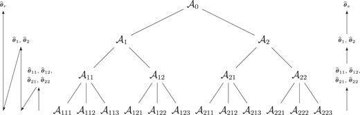
Example partition of |$\mathcal {A}_0$| with |$M=3$| resolutions. Schematic propagation steps for computation of |$\widehat{\boldsymbol{\theta }}_{k_1\ldots k_m}$| for recursive (left) and sequential (right) integration schemes.
Arguing as in Section 2.3.3, the computation and memory complexities of computing |$\widehat{\boldsymbol{\theta }}_s$| are |$O \lbrace NS_{k_1\ldots k_M}^3+ NM(pk_{\max })^3\rbrace$| and |$O \lbrace NS_{k_1\ldots k_M}^2+ NM(pk_{\max })^2 \rbrace$|, respectively. A consequence of the proof of Theorem 1 is that |$\widehat{\boldsymbol{\theta }}_s$| and |$\widehat{\boldsymbol{\theta }}_r$| are asymptotically equivalent. While |$\widehat{\boldsymbol{\theta }}_s$| may be computationally more advantageous, it requires that the MLEs from resolution M be close to |$\boldsymbol{\theta }_0$|, and may not perform as well as |$\widehat{\boldsymbol{\theta }}_r$| in finite samples.
3 SIMULATIONS
We investigate the finite sample performance of the proposed recursive and sequential MRRI estimators |$\widehat{\boldsymbol{\theta }}_r$| and |$\widehat{\boldsymbol{\theta }}_s$|. Unless otherwise specified, all simulations are on a Linux cluster using R linked to Intel’s MKL libraries with analyses at resolution M performed in parallel across |$\widetilde{K}=\prod _{m=1}^M K_m$| CPUs with 1 GB of RAM each. Standard errors and confidence intervals are calculated using the results in Theorem 1 and Corollary 1.
In the first set of simulations, we consider a |$S=400$|-dimensional square spatial domain |$\mathcal {S}= [1,20]^2=\lbrace \boldsymbol{s}_j\rbrace _{j=1}^{400}$|, |$\boldsymbol{s}_j \in \mathbb {R}^2$|, with |$N=10000$|. The Gaussian outcomes |$\lbrace y_i(\mathcal {S})\rbrace _{i=1}^N$| are independently simulated with means |$\lbrace \boldsymbol{X}^\top _i(\mathcal {S}) \boldsymbol{\beta }\rbrace _{i=1}^N$| and Gaussian spatial covariance function |$C_{\alpha }(\boldsymbol{s}_j, \boldsymbol{s}_{j^\prime }; \boldsymbol{\gamma })=\tau ^2 \exp \lbrace -\rho ^2 (\boldsymbol{s}_{j^\prime } - \boldsymbol{s}_j)^\top (\boldsymbol{s}_{j^\prime } - \boldsymbol{s}_j) \rbrace$|, with |$\boldsymbol{\beta }$|, |$\boldsymbol{\gamma }=(\tau ^2, \rho ^2)$| and nugget variance |$\sigma ^2$| specified below. The covariates |$\boldsymbol{X}_i(\boldsymbol{s}_j)=\boldsymbol{X}_i$| consist of an intercept and 2 nonspatially varying continuous variables independently generated from a Gaussian distribution with mean 0 and variance 4. The true value of the parameters is |$\boldsymbol{\beta }=(0.3,0.6,0.8)$|, |$\sigma ^2=1.6$|, |$\tau ^2=3$| and |$\rho ^2=0.5$|. To facilitate estimation, we estimate |$\boldsymbol{\theta }=\lbrace \boldsymbol{\beta }^\top , \log (\tau ^2), \log (\rho ^2), \log (\sigma ^2)\rbrace$| using |$\widehat{\boldsymbol{\theta }}_r$| and |$\widehat{\boldsymbol{\theta }}_s$|. We consider 5 recursive partitions of S. In Setting I, |$M=3$| with |$K_1=K_2=2, K_3=4$|; in Setting II, |$M=3$| with |$K_1=K_3=2$|, |$K_2=4$|; in Setting III, |$M=3$| with |$K_1=4$|, |$K_2=K_3=2$|; in Setting IV, |$M=2$| with |$K_1=2$|, |$K_2=8$|; in Setting V, |$M=4$| with |$K_1=K_2=K_3=K_4=2$|. Comparison of inference and run times across Settings I, II, and III shows the impact of the ordering of the recursive integration on the proposed procedure, while Settings IV and V investigate the impact of M and |$k_{\max }$| on inference and run time. Division of the spatial domain is based on nearest neighbors, as illustrated in the example of the supplement. We also estimate |$\boldsymbol{\theta }$| using 2 comparative approaches. Specifically, we compare to the partitioning approach (Part.) in Heaton et al. (2019) that evaluates the sum of the |$\widetilde{K}$| log-likelihoods at a grid of values of |$\tau ^2,\rho ^2$|, estimates |$\tau ^2,\rho ^2$| using the values that return the highest log-likelihood, then estimates |$\boldsymbol{\beta }$| and |$\sigma ^2$| using the least squares estimator and a sample variance, respectively; the implementation is modified directly from the code in Heaton et al. (2019). Asymptotic standard errors (ASEs) are estimated as the diagonal square root of the inverse variance of the score function. We also compare to the NNGP (Finley et al., 2019) using the 25 nearest neighbors; we implement this ourselves using sparse matrices in the R package "Rcpp" and parallelize over |$\widetilde{K}$| CPUs to make a fair comparison. Figure 2 plots the root mean squared error (RMSE), empirical standard error (ESE), and ASE averaged across 500 simulations for each parameter.
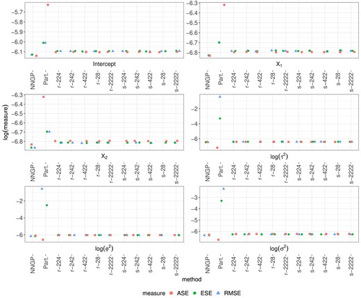
RMSE, ESE, and ASE for estimates of each parameter using NNGP, Part., |$\widehat{\boldsymbol{\theta }}_r$|, and |$\widehat{\boldsymbol{\theta }}_s$| in Settings I-V (r|$-224$|, r|$-242$|, r|$-422$|, r|$-28$|, r|$-2222$|, s|$-224$|, s|$-242$|, s|$-422$|, s|$-28$|, and s|$-2222$|, respectively) for the first set of simulations.
The near equality of RMSE and ESE in Figure 2 for our MRRI estimators |$\widehat{\boldsymbol{\theta }}_r$| and |$\widehat{\boldsymbol{\theta }}_s$| illustrates the near unbiasedness of our approach in large samples. Further, the near equality of ESE and ASE justifies the use of the asymptotic variance formula in Theorem 1 and Corollary 1 in large samples. Finally, negligible variation is observed across Settings I-V, illustrating the robustness of our approach to the chosen recursive or sequential integration scheme. The statistical inference properties of NNGP are similarly favorable, with the NNGP appearing slightly more efficient. The partitioning approach yields estimators of |$\boldsymbol{\beta }$| that are nearly unbiased in large samples, whereas the estimators of the covariance parameters show bias. Standard errors of the estimators are overestimated for |$\boldsymbol{\beta }$| and underestimated for the covariance parameters, which is problematic for statistical inference. This is further illustrated in Table 1, which reports the 95% confidence interval coverage (CP) for all estimators averaged across 500 simulations. Whereas CP reaches nominal levels for MRRI and NNGP, regression and covariance parameters are, respectively, overcovered and undercovered using Part.
95% CP in percentage for the first set of simulations: |$S=400$|, |$\boldsymbol{\theta }=\lbrace 0.3, 0.6, 0.8, \log (3), \log (0.5), \log (1.6)\rbrace$|.
| Method | |$K_1,\ldots ,K_M$| | Intercept | |$X_1$| | |$X_2$| | |$\log (\tau ^2)$| | |$\log (\rho ^2)$| | |$\log (\sigma ^2)$| |
|---|---|---|---|---|---|---|---|
| |$\widehat{\boldsymbol{\theta }}_r$| | 2, 2, 4 | 94 | 96 | 94 | 96 | 93 | 95 |
| 2, 4, 2 | 95 | 96 | 94 | 96 | 93 | 95 | |
| 4, 2, 2 | 94 | 95 | 95 | 96 | 93 | 95 | |
| 2, 8 | 94 | 96 | 94 | 96 | 93 | 95 | |
| 2, 2, 2, 2 | 95 | 96 | 94 | 96 | 93 | 95 | |
| |$\widehat{\boldsymbol{\theta }}_s$| | 2, 2, 4 | 94 | 96 | 94 | 96 | 93 | 95 |
| 2, 4, 2 | 95 | 96 | 94 | 96 | 93 | 95 | |
| 4, 2, 2 | 94 | 95 | 95 | 96 | 93 | 95 | |
| 2, 8 | 94 | 96 | 94 | 96 | 93 | 95 | |
| 2, 2, 2, 2 | 95 | 96 | 94 | 96 | 93 | 95 | |
| Part. | 100 | 100 | 100 | 0 | 0 | 0 | |
| NNGP | 95 | 95 | 95 | 96 | 96 | 96 |
Computing times are reported in Table 2. Using |$\widehat{\boldsymbol{\theta }}_s$| is faster than recursively updating weights with |$\widehat{\boldsymbol{\theta }}_r$|. In comparison, the partitioning and NNGP approaches are 212 and 467 times slower, respectively, than our estimator |$\widehat{\boldsymbol{\theta }}_s$| with |$K_1=4,K_2=K_3=2$|. We also observe the increased computational burden in Settings IV and V. This phenomenon is underpinned by the computation complexity orders of |$\widehat{\boldsymbol{\theta }}_r$| and |$\widehat{\boldsymbol{\theta }}_s$| derived in Sections 2.3.3 and 2.5, which show that computation is slower when M or |$k_{\max }$| are larger.
Mean elapsed time (Monte Carlo standard deviation) in seconds of |$\widehat{\boldsymbol{\theta }}_r$|, |$\widehat{\boldsymbol{\theta }}_s$|, NNGP and Part.
| Method | |$K_1,K_2,K_3$| | |$K_1,K_2,K_3$| | |$K_1,K_2,K_3$| | |$K_1,K_2$| | |$K_1,K_2,K_3,K_4$| | 16 CPUs |
|---|---|---|---|---|---|---|
| |$=2,2,4$| | |$=2,4,2$| | |$=4,2,2$| | |$=2,8$| | |$=2,2,2,2$| | ||
| |$\widehat{\boldsymbol{\theta }}_r$| | 0.80 (0.092) | 0.66 (0.060) | 0.66 (0.060) | 1.2 (0.86) | 0.97 (0.75) | |
| |$\widehat{\boldsymbol{\theta }}_s$| | 0.72 (0.084) | 0.60 (0.064) | 0.60 (0.064) | 1.2 (0.82) | 1.1 (1.2) | |
| NNGP | 276 (135) | |||||
| Part. | 127 (11) |
Across 500 simulations for the first set of simulations: |$S=400$|, |$\boldsymbol{\theta }=\lbrace 0.3, 0.6, 0.8, \log (3), \log (0.5), \log (1.6)\rbrace$|.
A second set of simulations with the same model and |$S=25600$| is presented in the supplement. There, we show that our MRRI estimators scale well when S grows. A third set of simulations in the supplement investigates the log-linear model with h the log function, |$S=900$|, and |$C_{\alpha }(\boldsymbol{s}_j, \boldsymbol{s}_{j^\prime }; \boldsymbol{\gamma })$| the exponential covariance function. Conclusions drawn from this simulation mirror those from the first 2 sets of simulations.
The fourth set of simulations mimics the data analysis of Section 4 with |$S=800$|. We consider 2 ROIs, |$\mathcal {S}_1=[1,20]^2=\lbrace \boldsymbol{s}_j\rbrace _{j=1}^{400}$| and |$\mathcal {S}_2=[21,40]^2=\lbrace \boldsymbol{s}_j\rbrace _{j=401}^{800}$|, |$\boldsymbol{s}_j \in \mathbb {R}^2$|. Defining |$\mathcal {S}=\mathcal {S}_1 \cup \mathcal {S}_2$|, the Gaussian outcomes |$\lbrace y_i(\mathcal {S})\rbrace _{i=1}^N$|, |$N=10000$|, are independently simulated with mean |$\lbrace \boldsymbol{1}\beta \rbrace _{i=1}^N$|, |$\beta =0$|, |$\boldsymbol{1}\in \mathbb {R}^S$| a vector of one’s, and the spatial covariance function in (1) with |$d=2$|. The spatial variance is modeled through |$\tau (\boldsymbol{s}_j, \boldsymbol{s}_{j^\prime })=\tau ^2$|, the spatial correlation is modeled through |$\boldsymbol{\rho }(\boldsymbol{s}_j) = \boldsymbol{\rho }_1 \mathbb {1}(\boldsymbol{s}_j \in \mathcal {S}_1) + \boldsymbol{\rho }_2 \mathbb {1}(\boldsymbol{s}_j \ \in \mathcal {S}_2)$|, and |$\boldsymbol{\gamma }=\lbrace \log (\tau ^2), \boldsymbol{\rho }^\top _1, \boldsymbol{\rho }^\top _2\rbrace ^\top \in \mathbb {R}^{1+2q}$|. Here, |$\boldsymbol{X}_i \in \mathbb {R}^q$| consists of an intercept and 2 nonspatially varying continuous variables independently generated from a Gaussian distribution with mean 0 and variance 1. The true values of the dependence parameters are set to |$\sigma ^2=1.6$|, |$\tau ^2=3$|, |$\boldsymbol{\rho }_1=(0.5,0.5,0.5)$|, and |$\boldsymbol{\rho }_2=(0.6,0.6,0.6)$|. We estimate |$\boldsymbol{\theta }=\lbrace \beta , \log (\tau ^2), \boldsymbol{\rho }^\top _1, \boldsymbol{\rho }^\top _2, \log (\sigma ^2)\rbrace$| using |$\widehat{\boldsymbol{\theta }}_s$| using the recursive partition of S with |$M=3$|: |$K_1=K_2=2$|, and |$K_3=4$|. Each set |$\mathcal {A}_{k_1\ldots k_m}$| at resolution m is a union of the nearest neighbors in |$\mathcal {S}_1$| and |$\mathcal {S}_2$| separately, so that each set |$\mathcal {A}_{k_1k_2k_3}$| consists of 25 locations from |$\mathcal {S}_1$| and 25 locations from |$\mathcal {S}_2$|, |$\mathcal {A}_{k_1k_2}$| consists of 100 locations from |$\mathcal {S}_1$| and 100 locations from |$\mathcal {S}_2$|, and so on. Analyses are parallelized across 16 CPUs with 2 GB of RAM each. Table 3 reports the RMSE, ESE, ASE, mean bias (BIAS), and CP of our MRRI estimator |$\widehat{\boldsymbol{\theta }}_s$| averaged across 500 simulations, where |$\boldsymbol{\rho }_j=(\rho _{j1},\rho _{j2},\rho _{j3})$|, |$j=1,2$|.
Simulation metrics of |$\widehat{\boldsymbol{\theta }}_s$| across 500 simulations for the fourth set of simulations: |$S=800$|, |$\boldsymbol{\theta }=\lbrace 0,\log (3),0.5,0.5,0.5,0.6,0.6,0.6,\log (1.6)\rbrace$|.
| Parameter | RMSE|$\times 10^3$| | ESE|$\times 10^3$| | ASE|$\times 10^3$| | BIAS|$\times 10^4$| | CP |$(\%)$| |
|---|---|---|---|---|---|
| |$\beta$| | 1.4 | 1.4 | 1.4 | −0.78 | 94 |
| |$\log (\tau ^2)$| | 1.1 | 1.1 | 1.1 | 0.44 | 96 |
| |$\rho _{11}$| | 1.9 | 1.9 | 1.9 | −0.57 | 94 |
| |$\rho _{12}$| | 1.9 | 1.9 | 1.8 | −0.88 | 94 |
| |$\rho _{13}$| | 1.9 | 1.8 | 1.8 | −1.80 | 93 |
| |$\rho _{21}$| | 1.9 | 1.9 | 1.9 | −0.35 | 94 |
| |$\rho _{22}$| | 1.9 | 1.9 | 1.9 | −1.20 | 95 |
| |$\rho _{23}$| | 1.9 | 1.9 | 1.9 | −0.49 | 94 |
| |$\log (\sigma ^2)$| | 1.2 | 1.2 | 1.2 | −0.51 | 96 |
Parallelizing over |$\widetilde{K}=16$| CPUs, mean elapsed time (Monte Carlo standard deviation) is 29 minutes (22 minutes). Simulation metrics in Table 3 are consistent with the results from the previous simulations: the RMSE, ESE, and ASE are approximately equal, the BIAS is negligible, and the CP reaches the nominal 95% level. Further, to illustrate the high statistical power of our approach, we perform a test of the hypotheses |$H_0: \rho _{12} = \rho _{22}$| versus |$H_A: \rho _{12} \ne \rho _{22}$| using the test statistic |$Z=(\widehat{\rho }_{12} - \widehat{\rho }_{22} -\rho _0)\lbrace \mathbb {V}(\widehat{\rho }_{12}) + \mathbb {V}(\widehat{\rho }_{22}) - 2\mbox{Cov}(\widehat{\rho }_{12}, \widehat{\rho }_{22})\rbrace ^{-1/2}$|, which follows an approximate standard normal distribution under |$H_0$| when |$\rho _0=0$|. In the context of the analysis of Section 4, this test evaluates whether ASD is associated with different spatial correlation in the left and right precentral gyri. Across the 500 simulations, the test rejects the null 100% of the time at level 0.05, illustrating the high statistical power of our approach. Using |$\rho _0=\rho _{12}-\rho _{22}$|, the type-I error rate is 3.6% across the 500 simulations.
4 ESTIMATION OF BRAIN FUNCTIONAL CONNECTIVITY
We return to the motivating neuroimaging application described in Section 1. Out of 1112 ABIDE participants, 774 passed quality control: 379 with ASD, 647 males (335 with ASD) and 127 females (44 with ASD), with mean age 15 years (standard deviation 6 years). The left and right precentral gyri form the primary motor cortex and are responsible for executing voluntary movements. They are two of the largest ROIs in the Harvard-Oxford atlas (FMRIB Software Library, 2018) with 1786 and 1888 voxels, respectively. Many individuals with ASD have motor deficits (Jansiewicz et al., 2006). Atypical connectivity within the left and right precentral gyri may indicate that these motor deficits are related to how these 2 brain regions coordinate movement. The preprocessing pipeline of rfMRI data has already been described by Craddock et al. (2013). Participant-specific data have been registered into a common template space such that voxel locations are comparable between participants.
Define |$\mathcal {S}_1=\lbrace \boldsymbol{s}_j\rbrace _{j=1}^{1888}$| and |$\mathcal {S}_2=\lbrace \boldsymbol{s}_j\rbrace _{j=1889}^{3674}$| the set of voxels in the right and left precentral gyri, respectively, and |$\mathcal {S}=\mathcal {S}_1 \cup \mathcal {S}_2$|. Voxels in the atlas outside the brain are assigned missing. Following the thinning described in Section 2.1, we obtain independent replicates |$y_i(\boldsymbol{s}_j)$| at |$S=3674$| voxel locations, |$i=1, \ldots , 75888$|. We refer to this dataset as the “primary” dataset; we compare estimates from this primary dataset to estimates from a secondary dataset, consisting of the excluded time points, with identical dimensions N and S. There is a priori no reason to believe that the data distribution differs across primary and secondary datasets, and so comparing results across both datasets will allow us to quantify robustness of our analysis, a notoriously difficult task in analyses of rfMRI data (Uddin et al., 2017).
Let |$\boldsymbol{X}_i$| be corresponding observations of |$q=5$| covariates for outcome i: an intercept, ASD status (1 for ASD, 0 for neurotypical), age (centered and standardized), sex (0 for male, 1 for female), and the age (centered and standardized) by ASD status interaction. We model |$\mu (\boldsymbol{s}_j; \boldsymbol{X}_i, \boldsymbol{\beta })=\beta$|, where |$\mu (\boldsymbol{s}_j; \boldsymbol{X}_i, \boldsymbol{\beta })$| is the mean rfMRI time series at voxel |$\boldsymbol{s}_j$|. The covariance |$C_{\alpha }(\boldsymbol{s}_{j^\prime }, \boldsymbol{s}_j; \boldsymbol{X}_i, \boldsymbol{\gamma })$| is that given in Equation (1) of Section 2.1 with |$d=3$| and |$\tau (\boldsymbol{s}_j, \boldsymbol{s}_{j^\prime })= \lbrace (\tau ^2_1)^{\mathbb {1}(\boldsymbol{s}_j \in \mathcal {S}_1) + \mathbb {1}(\boldsymbol{s}_{j^\prime } \in \mathcal {S}_1)} (\tau ^2_2)^{\mathbb {1}(\boldsymbol{s}_j \in \mathcal {S}_2) + \mathbb {1}(\boldsymbol{s}_{j^\prime } \in \mathcal {S}_2)} \rbrace ^{1/2}$|. As in Section 3, the correlation is modeled through |$\boldsymbol{\rho }(\boldsymbol{s}_j) = \boldsymbol{\rho }_1 \mathbb {1}(\boldsymbol{s}_j \in \mathcal {S}_1) + \boldsymbol{\rho }_2 \mathbb {1}(\boldsymbol{s}_j \ \in \mathcal {S}_2)$|. Thus, |$\boldsymbol{\gamma }=\lbrace \log (\tau ^2_1), \log (\tau ^2_2), \boldsymbol{\rho }_1^\top , \boldsymbol{\rho }_2^\top \rbrace \in \mathbb {R}^{2+2q}$| and |$\boldsymbol{\theta }=\lbrace \beta , \boldsymbol{\gamma }, \log (\sigma ^2)\rbrace$|, with |$\boldsymbol{\gamma }$| the parameter of interest describing the effect of covariates on functional connectivity. We interpret the effect of ASD on the correlation structure in detail in the supplement. An illustration of the correlation between ROIs for various values of |$\rho _{j2}, \rho _{j^\prime 2}$| is provided in the supplement.
The size of each (primary and secondary) outcome dataset is 15 GB. To overcome the computational burden of a whole dataset analysis, we estimate |$\boldsymbol{\theta }$| using the sequential estimator |$\widehat{\boldsymbol{\theta }}_s$|. To partition the 3-dimensional spatial domain, we recursively partition |$\mathcal {S}_1$| and |$\mathcal {S}_2$| separately into |$K_1=2$|, |$K_2=K_3=4$| disjoint sets based on nearest neighbors, |$M=3$|. The sets |$\mathcal {A}_{k_1\ldots k_m}$| consist of the union of the disjoint partition sets of |$\mathcal {S}_1$| and |$\mathcal {S}_2$| at each resolution |$m \in \lbrace 1, \ldots , M\rbrace$|. This strategy ensures that each |$\mathcal {A}_{k_1\ldots k_M}$| contains locations from both |$\mathcal {S}_1$| and |$\mathcal {S}_2$|, so that gyri-specific parameters |$\boldsymbol{\rho }_1,\boldsymbol{\rho }_2,\tau _1,\tau _2$| are identifiable in all sets |$\mathcal {A}_{k_1\ldots k_M}$|, |$k_M=1\ldots , K_M$|. A plot of the partitioning is provided in the supplement.
The analysis of the primary and secondary datasets takes 4.28 and 3.62 hours, respectively, when parallelized across 32 CPUs with 4 GB of RAM each; a comparison of these run times is detailed in the supplement. We attempted to obtain the MLE using either the whole primary or secondary dataset by supplying the value of |$\widehat{\boldsymbol{\theta }}_s$| as a starting value. The estimation required more than 170 GB of RAM and terminated without completing after 190 hours. The standard deviation (s.d.) of block-specific estimates of |$\log (\sigma ^2)$| across the |$K_1K_2K_3=32$| blocks is 0.401 and 0.399 in the primary and secondary datasets, respectively, supporting our assumption that |$\sigma ^2$| does not depend on |$\boldsymbol{s}$|; complete summaries are available in the supplement. The estimated effect and s.d. of the intercept, ASD status, age, sex, and age by ASD status interaction are reported in Table 4. In the primary dataset, the estimates (s.d.) of |$\beta$|, |$\log (\sigma ^2)$|, |$\log (\tau ^2_1)$| and |$\log (\tau ^2_2)$| are, respectively, |$-0.00537$| (|$2.03\times 10^{-4}$|), |$-4.05$| (|$3.90\times 10^{-4}$|), |$-0.108$| (|$2.53\times 10^{-4}$|), and |$-0.0699$| (|$2.48\times 10^{-4}$|). In the secondary dataset, the estimates (s.d.) of |$\beta$|, |$\log (\sigma ^2)$|, |$\log (\tau ^2_1)$| and |$\log (\tau ^2_2)$| are, respectively, |$-0.00609$| (|$2.03\times 10^{-4}$|), |$-4.05$| (|$3.88\times 10^{-4}$|), |$-0.111$| (|$2.51\times 10^{-4}$|), and |$-0.0709$| (|$2.46\times 10^{-4}$|). As expected, estimates of |$\beta$| are close to 0 and estimates of |$\sigma ^2+\tau ^2_j$| are close to 1 due to the centering and standardizing. The cosine similarity between standardized estimates of |$\boldsymbol{\theta }$| in the primary and secondary datasets, that is, the cosine of the angle between the 2 standardized vectors |$\widehat{\theta }_{q}/\lbrace \mathbb {V}(\widehat{\theta }_{q}) \rbrace ^{1/2}$|, |$q=1, \ldots , 14$|, is 0.999994, indicating a high degree of agreement between the standardized vectors.
Estimated covariate effects and s.d. in the primary and secondary datasets.
| |$\boldsymbol{\rho }_1$| | |$\boldsymbol{\rho }_2$| | |||
|---|---|---|---|---|
| Covariate | Estimate | s.d.|$\times 10^4$| | Estimate | s.d.|$\times 10^4$| |
| Primary dataset | ||||
| Intercept | 0.569 | 1.44 | 0.561 | 1.42 |
| ASD status | −0.00676 | 1.32 | −0.0050 | 1.27 |
| Age | −0.0222 | 1.07 | −0.0120 | 0.932 |
| Sex | 0.0362 | 1.79 | 0.0655 | 1.72 |
| Age by ASD status interaction | −0.00310 | 1.38 | −0.00386 | 1.25 |
| Secondary dataset | ||||
| Intercept | 0.568 | 1.43 | 0.562 | 1.41 |
| ASD status | −0.00511 | 1.32 | −0.00472 | 1.27 |
| Age | −0.0211 | 1.07 | −0.0118 | 0.931 |
| Sex | 0.0341 | 1.78 | 0.0643 | 1.72 |
| Age by ASD status interaction | −0.00503 | 1.38 | −0.00591 | 1.25 |
From a practical perspective, estimates and their standard errors are virtually identical across primary and secondary datasets. Two-sample Z-tests, however, mostly reject the null that elements of |$\boldsymbol{\theta }$| are equal in both datasets at the typical 0.05 level: this is a feature of the sample size and the high power of the test, rather than of true underlying differences between the 2 datasets, and illustrates well the challenges of robustness in analyses of rfMRI data. We calibrate the |$\alpha$|-level of hypothesis testing procedures in our analysis by borrowing ideas from knock-offs (Barber and Candès, 2015). We estimate a data-dependent type-I error rate threshold as the 5% quantile of the observed p-values of the 2-sample tests of equality between parameters in primary and secondary datasets. The Gaussian critical value corresponding to this 5% quantile is |$z_{\mbox{{crit}}}=9.87$|.
Armed with this robust critical value, we evaluate whether the ASD main and interaction effects are significantly different across the 2 brain regions. We perform a test of the hypotheses |$H^m_0: \rho _{12}=\rho _{22}$| versus |$H^m_A: \rho _{12} \ne \rho _{22}$| and |$H^i_0: \rho _{15}=\rho _{25}$| versus |$H^i_A: \rho _{15}\ne \rho _{25}$| using the test statistic Z in Section 3, where |$\rho _{j2}$| and |$\rho _{j5}$| are the ASD main and interaction effects, respectively, in ROI |$\mathcal {S}_j$|, |$j=1,2$|. The test statistic for |$H^m_0$| versus |$H^m_A$| takes a value of 13.99 and 3.04 in the primary and secondary datasets, respectively; since we reject |$H^m_0$| in the primary but not the secondary dataset, we conclude that the main ASD effect is not significantly different in the correlation structure of both brain regions. The test statistic for |$H^i_0$| versus |$H^i_A$| takes a value of 6.14 and 7.13 in the primary and secondary datasets, respectively, and we conclude that the ASD by age interaction effect is not significantly different in the correlation structure of both brain regions. An analysis that excludes the age by ASD status interaction is included in the supplement and agrees with this analysis.
Summaries of distances |$d_{jj^\prime }=(\boldsymbol{s}_{j^\prime } - \boldsymbol{s}_j)^\top (\boldsymbol{s}_{j^\prime } - \boldsymbol{s}_j)$| are provided in the supplement. For a male participant of mean age (15.13 years), the estimated correlation structures between the right and left precentral gyri, within the right precentral gyrus, and within the left precentral gyrus, for a participant with and without ASD are, respectively, |$0.915 \exp (- 1.83 d_{jj^\prime })$| and |$0.915 \exp (- 1.86 d_{jj^\prime })$|, |$0.898 \exp (- 1.85 d_{jj^\prime })$| and |$0.898 \exp (- 1.89 d_{jj^\prime })$|, and |$0.932 \exp (- 1.82 d_{jj^\prime })$| and |$0.932 \exp (- 1.84 d_{jj^\prime })$|. ASD manifests as hyperconnectivity within and between the right and left precentral gyri. These findings concur with those of Nebel et al. (2014). These results also concur with a less powered analysis that averages each participant’s rfMRI time series at each voxel, then regresses the participants’ Pearson correlation between the right and left precentral gyri onto an intercept, ASD status, age, sex, and the age by ASD status interaction. Estimates (s.d.) of covariate effects from this analysis are 0.726 (0.00759), |$-0.0457$| (0.0101), 0.0159 (0.00745), |$-0.0111$| (0.0137), and |$-0.00293$| (0.0101). Only the intercept, ASD status, and age effects are significant at level 0.05, highlighting the superior power of our spatial approach.
5 DISCUSSION
The proposed MRRI estimators depend on the choice of the recursive partition of |$\mathcal {S}$|. We have suggested that this partitioning be performed such that |$S_{k_1\ldots k_m}$| and |$K_m$|, |$m=1, \ldots , M$| are relatively small compared to |$S_0$| and shown through simulations that this leads to desirable statistical and computational performance. Nonetheless, the GMM is known to underestimate the variance of estimators when |$K_m$| is moderately large relative to N (Hansen et al., 1996). Thus, special care should be taken to ensure |$K_m$| is relatively low-dimensional.
In this paper, we have allowed |$\boldsymbol{\theta }$| to vary spatially under the constraint that it can be consistently estimated using subsets of the spatial domain |$\mathcal {S}$|. While we have assumed that |$\sigma ^2$| does not depend on |$\boldsymbol{s}$|, a model that allows |$\sigma ^2$| to depend on |$\boldsymbol{s}$| can easily be fitted in our framework under this constraint. Other settings may consider a setting in which each subset is modeled through its own, subset-specific parameter. Future research should focus on the development of recursive and sequential integration rules for this setting with partially heterogeneous parameters |$\boldsymbol{\theta }$| following, for example, the work of Manschot and Hector (2022) and Hector and Reich (2024) in spatially varying coefficient models. Such extensions would allow parameters such as the nugget variance |$\sigma ^2$| to vary with |$\boldsymbol{s}$|. A priori, these extensions should follow from zero-padding the weight matrices in Equations (4) and (6).
While our approach was motivated by a comparison of functional connectivity between participants with and without ASD, the proposed methods are generally applicable to Gaussian process modeling of high-dimensional images. Our ABIDE analysis has primarily focused on modeling correlation between the left and right precentral gyri as a function of the within-ROI correlations. This analysis is suitable when within-ROI correlation is of primary interest. Extensions that model the between-ROI correlation through a more flexible covariance structure are of interest but beyond the scope of the present work.
ACKNOWLEDGMENTS
The authors thank the reviewers and associate editor for their valuable feedback, which led to an improved manuscript. The authors also thank the ABIDE study organizers and members.
FUNDING
E.C.H. and B.J.R. were supported by the National Science Foundation grant DMS 2152887.
CONFLICT OF INTEREST
None declared.
DATA AVAILABILITY
ABIDE I data usage is unrestricted for noncommercial research purposes. To obtain access to ABIDE I data, complete registration with NITRC at nitrc.org/ir, then register with the 1000 Functional Connectomes Project at nitrc.org/projects/fcon_1000. Data access is also described at fcon_1000.projects.nitrc.org/ indi/abide/abide_I.html.
References
 Open Materials
