Causal inference using multivariate generalized linear mixed-effects models Open Access

ABSTRACT

1 INTRODUCTION

Precision medicine (Rosen et al., 2019) strives to improve clinical decision-making for the current patient by systematically learning from prior patient outcomes obtained from both experimental and observational studies. Our motivating application is to study the effectiveness of an immunosuppressant medication, mycophenolate mofetil (MMF; Omair et al., 2015), in scleroderma patients using longitudinal clinical data from the Johns Hopkins Scleroderma Center Research Registry. Scleroderma is a rare multisystem autoimmune disease marked by exaggerated fibrosis, vasculopathy, and derangements of the immune system. Based on limited observational and clinical trial data, MMF is the current standard of care for patients with active diffuse cutaneous systemic sclerosis and/or interstitial lung disease (ILD). However, the trajectory of scleroderma is quite heterogeneous; while many patients have radiographic evidence of ILD, a relatively small percentage have life-threatening progressive lung disease. Given this clinical variability and the side effects of MMF, such as the increased risk of infection and gastrointestinal adverse effects, it remains unknown how to best deploy the treatment to the right patient at the right time. There is currently no universally accepted treatment for the disease’s skin thickening due to the paucity of studies.

We aim to compare the efficacy of MMF-containing versus MMF-free treatment regimens for skin and lung measurements in patients who have demonstrated tolerance to MMF. There are multiple practical challenges: treatment assignment is not randomized based on measured factors, biomarkers are measured irregularly, missingness patterns may be informative about biomarker values, and natural heterogeneity among subjects exists beyond what the observables can explain. To tackle these issues, we use a Bayesian approach under the potential outcomes framework (Rubin, 1974), which defines causal effect as a comparison of potential outcomes for the same set of subjects under different treatment regimes.

A primary factor in evaluating treatment efficacy is subject heterogeneity from unmeasured factors in treatment assignment and biomarker dynamics. Unmeasured factors like patient frailty, patients’ willingness to be treated, and potential risk of adverse effects from treatment can confound disease progression and influence treatment decisions. When unobserved permanent components exist, subjects with similar observables may have heterogeneous distributions of responses (Heckman and Willis, 1977). Causal inference methods often assume unconfoundedness, that is, treatment assignment is independent of the potential outcomes conditional on observed variables. The existence of unmeasured factors that may confound the treatment assignment and biomarker dynamics violates this fundamental assumption and thus undermines these methods, including g-estimation (Robins, 1986), structural nested models (He et al., 2015), history-restricted marginal structural models (Neugebauer et al., 2007), and longitudinal targeted maximum likelihood estimation (Van der Laan et al., 2011). Imai and Kim (2019) used unobserved effects models (UEM) in matching to estimate the contemporaneous treatment effect, reducing time-invariant unmeasured confounding by having each subject acting as their own control. Allison et al. (2017) discussed the drawback of UEM; due to its assumption of strict exogeneity (the expectation of random errors is zero conditional on covariates and unobserved time-invariant confounders), it is difficult to simultaneously address biases from reverse causation and time-dependent confounding, which are common in studying time-varying treatments.

We account for the unmeasured patient heterogeneity in both treatment assignment and biomarker dynamics via multivariate generalized linear mixed-effects models (MGLMM; Zeger and Karim, 1991). UEM and MGLMM seem to have similar model specifications but rely on fundamentally different assumptions. The former do not make distributional assumptions about subject-specific effects, whereas the latter do for borrowing information from the population. The subject-specific effects represent between-subject heterogeneity caused by unobserved factors (Schwartz and Stone, 2007). Furthermore, MGLMM describe the within-subject dependence in the time-varying dependent variables, improving parameter estimation efficiency. Due to the nonlinear link functions, fixed-effects coefficients in MGLMM no longer represent marginal causal effect based on potential outcomes even when all covariates are exogenous (Heagerty, 1999).

To estimate the marginal causal effect for comparing treatment regimes with MGLMM on the entire population and subgroups, we use the Bayesian g-computation algorithm (GCA). Arjas and Parner (2004) provided an early version of the Bayesian GCA without utilizing the potential outcomes framework. They presented a rigorous discussion on the role of unmeasured confounder(s) in the case of sequential treatments and suggested that the comparison of treatment regimes can be achieved by comparing the simulated values obtained from the respective predictive distributions using Monte Carlo simulation with the same random seed. Arjas and Saarela (2010) articulated the idea and proposed that when the decision space is small, the optimal regime can be determined by modeling the longitudinal distribution of the data and comparing the posterior predictive distributions of the potential outcomes under different treatment regimes. Saarela et al. (2015) gave a Bayesian justification for the GCA and proposed a weighting scheme under the presence of latent individual-level characteristics to remove observed confounding that is not involved in the treatment regimes. Keil et al. (2018) proposed to simulate potential outcomes under a treatment path from the joint distribution of time-varying confounders and outcomes conditional on patient history.

Standard g-estimation methods produce biased effect estimates when unmeasured confounders are present, as unobserved potential outcomes are not missing at random. From a sensitivity analysis perspective, Yang and Lok (2018) assumed a nonidentifiable bias function quantifying the impact of unmeasured confounding on the average potential outcome under structural nested mean models. Sitlani et al. (2012) and Qian et al. (2020) compared treatment paths that differ only at a single point in time and discussed likelihood decomposition, which supports the causal interpretation of the fixed-effects coefficients estimated from a linear mixed-effects model. Shardell and Ferrucci (2018) incorporated joint mixed-effects models in GCA to estimate population average effect of treatment regimes over time.

Our method belongs to the class of Bayesian causal inference, which has developed substantially in recent years and typically assumes the exchangeability or unconfoundedness of the modeled observable quantities. Stephens et al. (2023) explored the use of propensity scores (PS) in Bayesian causal analysis. Davis et al. (2019) applied a Bayesian approach to jointly estimate a propensity score and outcome model with spatial random effects, then inserted predictions into a frequentist doubly robust estimator to account for spatial heterogeneity. Villain et al. (2019) adopted a quasi-Bayesian approach to forecast the dynamics of outcomes using a system of ordinary differential equations with random effects, and compared various outcome-based protocols of dynamical treatment adaptation. To account for unmeasured confounding in Bayesian spatial modeling, Nobre et al. (2023) used a plug-in 2-step approach to use propensity score in a multilevel model with shared random effects.

In this paper, we relax the unconfoundedness assumption and use MGLMM for causal comparison of treatment paths, accounting for unmeasured time-invariant factors as latent subject heterogeneity in treatment assignments, longitudinal outcomes, and time-varying confounders. The proposal enables us to assess the sensitivity of the longitudinal causal effect estimation to different distributions of unobserved treatment heterogeneity while allowing time-invariant unmeasured confounding. We aim to synthesize sample evidence pertinent to clinical decisions of an individual and account for the dynamic progression of individual trajectories while addressing unobserved permanent factors in selection bias and adhering to the generic causal inference ideology of only using the past to infer the present. Existing works on causal inference using mixed-effects models often marginalize latent components and identify causal estimand as a function of the treatment path, covariates, and fixed-effects coefficients. While the unobserved stable trait factors influencing disease progression remain constant over time, our proposal dynamically updates the information relevant to these factors based on a subject’s accumulating observed or counterfactual history. Our proposal engages the treatment assignment model to bridge the gap between the confoundedness in selection bias and the heterogeneity of patients’ dynamic disease progression.

2 NOTATION AND MODEL

We consider a longitudinal study with sequentially assigned treatments and with time-invariant unobserved random effects in both biomarkers and treatment assignment. Figure 1 is a causal graph in which an arrow represents a causal relationship (single arrow) or covariance (no arrow); a missing arrow implies zero influence or zero covariance. There is a multivariate stochastic process, |$\lbrace (Y_t, M_t, A_t): t\ge 0\rbrace$|⁠, where |$Y_t$|⁠, |$M_t$|⁠, and |$A_t$| represent the outcome process, time-dependent measured confounders, and sequential binary treatment, respectively. The confounders can be affected by previous exposure and can influence future outcomes and treatment assignments. Let |$\overline{Y}_{i, t_1:t_2}$|⁠, |$\overline{M}_{i, t_1:t_2}$|⁠, and |$\overline{A}_{i, t_1:t_2}$| be the longitudinal biomarkers, confounders, and interventions from |$t_1$| to |$t_2$| for subject |$i$|⁠, |$i=1,\ldots , N$|⁠. At time |$t$|⁠, clinician decides on |$A_{i, (t+1)}$| based on clinical history up to time |$t$|⁠, that is, past treatment path |$\overline{A}_{i,0:t}$| and measurement history |$\mathcal {H}_{i,t+1}=(V_i,\overline{Y}_{i,0:t},\overline{M}_{i,0:t})$|⁠, where |$V_i$| contains baseline information. The updated clinical history, |$(\mathcal {H}_{it},\overline{A}_{i,0:(t+1)})$|⁠, that includes the most recent treatment decision, is then the observable information for explaining the dynamics of |$(Y_{i,t+1}, M_{i,t+1})$|⁠.

FIGURE 1

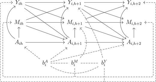
Directed acyclic graph (DAG) for the generalized linear mixed model displaying temporal order of the observed variables and time-invariant unmeasured heterogeneity in both treatment assignment and biomarker dynamics. Baseline characteristics |$V_i$| is excluded from the figure for simplicity.

Open in new tabDownload slide

This paper focuses on monotone treatment assignment, where each subject receives 1 initiation and treatment constants afterward. Without loss of generality, we consider the case where the outcomes are continuous and the time-dependent confounders summarize subject visit patterns. The latter are binary variables that indicate whether longitudinal measurements were updated during each time interval. The MGLMM below describe the data-generating mechanism as illustrated in Figure 1. Let |$\phi ^X(\cdot )$| be a function of the variables in |$(\cdot )$| for modeling variable |$X$|⁠. The continuous outcomes have the following specification:

where |$t=1,\ldots ,T$|⁠, |$\lambda _Y$| is the scalar link function for each outcome, |$\phi _A(\overline{A}_{i,0:t})$| is a function of dosage information for person |$i$| at time |$t$| with maximum dose |$K$|⁠, and |$b^Y_i = (b^Y_{i0},b^Y_{i1})$| is outcomes’ random effects for person |$i$|⁠. Outcome model parameters are |$\theta ^Y = (\beta ^Y_1,\beta ^Y_2, \sigma )$|⁠, where |$\sigma$| is the standard deviation of outcome distribution, and |$\psi ^Y_i$| is the standard stochastic randomness following a mean zero distribution, for example, |$\sigma \psi ^Y_i \sim N(0,\sigma ^2)$|⁠. Treatment initiation is modeled as

where |$\lambda _A$| is the link function, |$\theta ^A=(\beta ^A_1,\beta ^A_2)$|⁠, and |$b^A_i = b^A_{i0}$| is the random effect. For the monotone binary treatment assignment process, the variance of |$b^A_{i0}$| is not identifiable, and the model estimation requires it to be prespecified. With a binary dependent variable, the randomness satisfies |$\psi ^A_{it} \sim U(0,1)$| and indicates a realization of |$A_{it}$| via |$ \mathbb {1}\lbrace \psi ^A_{it} \le \lambda ^{-1}_A(\eta ^A_{it})\rbrace$| when |$A_{i,t-1} = 0$|⁠. We recognize that the distribution of the heterogeneity in treatment assignment, |$b^A_i$|⁠, is not fully identifiable from the observed data when the assignment is not a recurrent process. For identifiability, we specify the value and do sensitivity analysis on the variance of |$b^A_i$|⁠. For time-dependent confounders |$M_{it}$|⁠, the model specification is

where |$\theta ^M=(\beta ^M_1,\beta ^M_2)$|⁠, |$\lambda _M$| is the link function, and |$b^M_i = (b^M_{i0},b^M_{i1})$| is the random effects. In the application, |$M_{it}$| represents whether or not the outcomes were updated. Random errors |$(\psi ^Y_{it},\psi ^M_{it},\psi ^A_{it})$| are i.i.d and independent of |$b_i$|⁠; they characterize the distributional uncertainty in counterfactuals. We use the same randomness for causal estimation across different treatment regimes so that projected potential outcomes are comparable and reproducible.

Model components (1), (2), and (3) are connected through a covariance structure between the random effects, |$b_i = (b^Y_i,b^M_i,b^A_i)^T\sim MVN(0, G_i)$|⁠. We assume multivariate normal because it is mathematically convenient, easily facilitates association among the components, and enables a simple form of shrinkage for subject-level estimates, allowing individual inference to borrow strength from population data even for patients with few or no observations. The proposal and code can be modified for any multivariate distribution of random effects. Considerable literature (McCulloch and Neuhaus, 2011) showed that population average parameters and subject-level estimates are generally unbiased under mis-specified random effects distributions, except in extreme cases. A potential solution to address bias concerns is to use flexible distributions like mixtures to capture multi-modal or skewed distributions (Noma et al., 2022), which is beyond the scope of this work.

In our application, we assume |$G_i$| to be the same across subjects, that is, |$b_i \sim MNV(0, G)$|⁠. With sufficient sample size, |$G_i$| can also be allowed to vary with covariates. These random effects are interpreted as unobserved time-invariant subject-specific unmeasured stable traits that influence the clinical trajectories and treatment assignment processes directly via random intercepts or indirectly through the effect of factors via random slopes. Specifically, |$b^A_i$| is the unmeasured static heterogeneity in treatment assignment, such as a patient’s frailty that is not recorded in the observational data. In most cases, model parameters in MGLMM do not have a population-level causal interpretation due to the random effects, with an exception described in the supplementary material. Without loss of generality, we assume that |$\psi ^Y_{it} \sim N(0,1)$|⁠, identity link for |$\lambda _Y$|⁠, and logit link for |$\lambda _A$| and |$\lambda _M$|⁠.

3 BAYESIAN G-COMPUTATION WITH MGLMM

3.1 Causal quantities and target estimand

A treatment regime dynamically defines a patient’s present treatment status as a function |$q(\cdot )$| of the observed or counterfactual clinical history, that is, given a past treatment path and measurement history up to time |$t$|⁠, |$(\overline{A}_{i,0:(t-1)},\mathcal {H}_{it})$|⁠. The treatment sequence under regime |$q$| is sequentially determined by |$a_t(q) = q(\overline{A}_{i,0:(t-1)},\mathcal {H}_{it})$|⁠. For any variable |$X$|⁠, |$X(q)$| represents the value of |$X$| had the individual received treatment under regime |$q$|⁠. We define |$\overline{Y}_{i,0:t}(q)$|⁠, |$\overline{M}_{i,0:t}(q)$|⁠, and |$\overline{a}_{0:t}(q) = (a_1(q),\ldots ,a_t(q))$| as the counterfactual longitudinal trajectories of outcomes, confounders, and treatment path under regime |$q$|⁠, and write the counterfactual measurement history under regime |$q$| up to before time |$t$| as |$\mathcal {H}_{it}(q) = \lbrace V_i, \overline{Y}_{i,t-1}(q),\overline{M}_{i,t-1}(q)\rbrace$|⁠.

The heterogeneity in treatment assignment, |$b^A_i$|⁠, represents possible clinician-observed but unrecorded signals or stable trait factors that are not captured by data but are relevant to clinicians’ judgments about the potential outcomes of their patients. To account for potential time-invariant unmeasured confounding that may occur naturally in the process of treating patients in clinic, we stratify the causal estimation based on treatment assignment heterogeneity. Given a specific regime of interest, |$q$|⁠, and the unobserved time-invariant heterogeneity in treatment assignment, |$b^A_i$|⁠, we identify the joint distribution of a future |$\tau$| days of counterfactual trajectories conditional on observed history up to a present time |$h$|⁠,

Based on Equation 4 and GCA, we identify causal effects from the expectation of counterfactual outcomes that are functions of the fixed-effects parameters and the time-evolving estimates of |$(b^Y_i, b^M_i)$| by integrating over observed or counterfactual histories under treatment regimes.

Target quantity is the conditional mixed average treatment effect (CMATE; Li et al., 2022) within a target subgroup |$T$| characterized by |$\lbrace V_i, \overline{A}_{i,0:h_i}, \overline{Y}_{i,0:h_i}, \overline{M}_{i,0:h_i}\rbrace _{i\in T}$|⁠, in which person |$i$| contributes history information to the subgroup up to time |$h_i$|⁠. Our application considers |$T$| as containing follow-up information prior to MMF usage from scleroderma patients who were observed to be treated with MMF. Let |$\widehat{P}_T$| be the empirical distribution based on the observed values in subgroup |$T$|⁠, then the target quantity CMATE is defined as

where |$N_T$| is the number of individuals in subgroup |$T$|⁠. Replacing the empirical distribution with the corresponding population distribution yields the population version of CMATE, which is a longitudinal extension of conditional average treatment effect (ATE) and is realized by jointly modeling all the variables involved in the definition of subgroup |$T$|⁠.

3.2 Assumptions and method

In this section, we describe the assumptions and explain the procedure for estimating CMATE, which jointly models multivariate time-varying components while accounting for the accumulation of individual information over time via time-evolving updates of |$(b^Y_i, b^M_i)$|⁠. For simplicity, we leave out subscript |$i$| for the following discussion. To show that Equation 4 can be identified, we make the following assumptions. For |$t = 0,\ldots , T$|⁠,

1. Consistency: |$\overline{Y}_{0:t} \overset{d}{=} \overline{Y}_{0:t}(q)$| and |$\overline{M}_{0:t} \overset{d}{=} \overline{M}_{0:t}(q)$| if |$\overline{A}_{0:t} = \overline{a}_{0:t}(q)$|⁠;

2. Positivity: |$P(A_{t+1} = a_{t+1}(q) |V, \overline{A}_{0:t} = \overline{a}_{0:t}(q),\overline{Y}_{0:t}, \overline{M}_{0:t}, b^A_i) \gt 0$| with probability 1 for |$t \ge 0$|⁠;

3. Sequential exchangeability given |$b^A_i$|⁠: for |$\tau \gt 0$|⁠,

   $$\begin{eqnarray} &&P(\overline{Y}_{(t+1):(t+\tau )}(q), \overline{M}_{(t+1):(t+\tau )}(q) |V, A_{t+1}, \overline{A}_{0:t}\\ &&\quad= \overline{a}_{0:t}(q), \overline{Y}_{0:t}, \overline{M}_{0:t}, b^A_i)\\ &&\quad= P(\overline{Y}_{(t+1):(t+\tau )}(q), \overline{M}_{(t+1):(t+\tau )}(q) |V,\overline{A}_{0:t}\\ &&\quad= \overline{a}_{0:t}(q), \overline{Y}_{0:t}, \overline{M}_{0:t}, b^A_i). \end{eqnarray}$$

We extend the classic assumption of sequential exchangeability (Greenland and Robins, 1986) to condition on the unobserved time-invariant heterogeneity in treatment assignment, which is quantified by the random effect |$b^A_i$| in model (2). In practice, the heterogeneity in treatment assignment may be attributable to patients’ willingness to be treated, the potential risk of adverse effects from treatment, and the clinician’s perception of treatment. Under these assumptions and that models (1), (2), and (3) are correctly specified, Equation 4 can be identified as below (see Web Appendix A for details)

In Figure 2, we use a single-world intervention graph (SWIG; Richardson and Robins, 2013) to display the independencies that lead to Equation 6 and show the counterfactual dependencies that would exist if we set the treatment path to that under regime |$q$|⁠. The graph is constructed by splitting the treatment nodes |$\overline{A}_{i,(h+1):(h+\tau )}$| of the causal diagram in Figure 1 and replacing all descendants of the assigned treatment with their potential outcomes, marking all counterfactuals in red. The conditional sequential exchangeability assumption is demonstrated in the SWIG by d-separation between the counterfactual trajectories |$(\overline{Y}_{(h+1): (h+\tau )}(q),\overline{M}_{(h+1):(h+\tau )}(q) )$| and |$A_{i,h+1}$| conditional on |$(\overline{A}_{0:h}, \overline{Y}_{0:h}, \overline{M}_{0:h}, b^A_i)$|⁠. If |$b^A_i$| is not controlled for, selection bias would be induced by paths |$A_{i,h+1}\leftarrow b^A_i\leftrightarrow b^Y_i \rightarrow Y_{i,h+1}(q)$| and |$A_{i,h+1}\leftarrow b^A_i\leftrightarrow b^M_i \rightarrow M_{i,h+1}(q)$|⁠, while stratifying on |$b^A_i$| blocks these paths. Variables inside rectangles of Figure 2 are quantities involved in Equation 6 that are relevant to the time-evolving update of |$(b^Y_i, b^M_i)$|⁠. At each time point, the distribution of |$(b^Y_i, b^M_i)$| can be derived based on information backflow from observed or counterfactual biomarkers’ history, resulting in a sequential update of these subject-specific unobserved permanent traits. The counterfactual treatment statuses |$\overline{a}_{it} (q)$|⁠, |$t\in [h+1,h+\tau ]$|⁠, do not contribute to the sequential update of |$(b^Y_i, b^M_i)$| because they are hypothesized and generate no additional information beyond the definition of the regime of interest.

FIGURE 2

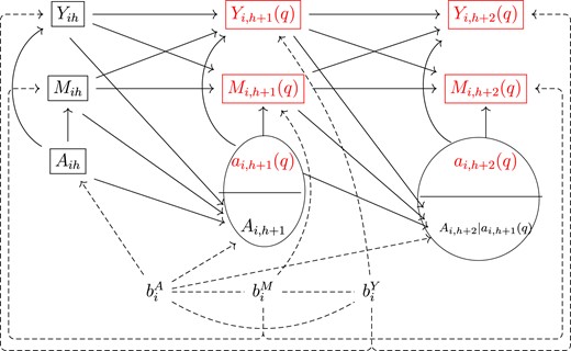
Single-world intervention graph (SWIG) for displaying the independencies that lead to Equation 6 and the counterfactual dependencies that would exist if we set the treatment path to that under a regime |$q$|⁠.

Open in new tabDownload slide

At each time |$s \in [h, h+\tau )$|⁠, Monte Carlo simulation of counterfactual outcomes and confounders |$(Y_{s+1}(q), M_{s+1}(q))$| based on Equation 6 involves integration over |$P(b^Y_i, b^M_i | V,\overline{A}_{0:h}, \overline{Y}_{0:s}, \overline{M}_{0:s}, b^A_i)$|⁠, an updated conditional posterior distribution of |$(b^Y_i, b^M_i)$|⁠. Note that the trajectories being conditioned on, |$(\overline{Y}_{0:s}, \overline{M}_{0:s})$|⁠, is equivalent to |$(\overline{Y}_{0:h},\overline{Y}_{(h+1):s}(q), \overline{M}_{0:h},\overline{M}_{(h+1):s}(q))$| in distribution, which is a combination of observed and counterfactual variables. The counterfactual trajectories |$(\overline{Y}_{(h+1):s}(q), \overline{M}_{(h+1):s}(q))$| follow the distribution |$ \prod ^{s-1}_{s = h} P( Y_{s+1} , M_{s+1}| V, \overline{A}_{0:(s+1)} = \overline{a}_{0:(s+1)}(q), \overline{Y}_{0:s}, \overline{M}_{0:s}, b^A_i)$| under regime |$q$| and treatment assignment heterogeneity |$b^A_i$|⁠, as implied by Equation 6. The sampling of |$(b^Y_i, b^M_i)\sim P(b^Y_i, b^M_i | V,\overline{A}_{0:h}, \overline{Y}_{0:s}, \overline{M}_{0:s}, b^A_i)$| is computationally expensive due to the nonlinear link functions in the MGLMM. We use the following general strategy: first, calculate the Laplace approximation of the posterior distribution |$(b^Y_i, b^M_i, b^A_i| V,\overline{A}_{0:h}, \overline{Y}_{0:s}, \overline{M}_{0:s})$|⁠, denoted by |$MVN(\hat{b}_i, V)$|⁠, and then sample the heterogeneities via the corresponding conditional distribution, |$(b^Y_i, b^M_i)|b^A_i$|⁠, with |$b^A_i$| set to a fixed value. The procedure is illustrated in Web Appendix B. We provide in Web Appendix C the pseudocode for generating posterior samples of counterfactual trajectories from |$P(\overline{Y}_{(h+1): (h+\tau )}(q),\overline{M}_{(h+1):(h+\tau )}(q) |$|  |$ V, \overline{A}_{0:h}, \overline{Y}_{0:h}, \overline{M}_{0:h}, b^A_i)$| based on Equation 6.

We have been holding |$b^A_i$| fixed thus far in our discussion. Conditional mixed average treatment effect expressed in Equation 5 is the marginal subgroup ATE, marginalizing over treatment assignment heterogeneity. Therefore, we can obtain the integrand in Equation 5 by integrating |$\mathbb {E}(Y_{h+\tau }(q)|V, \overline{A}_{0:h}, \overline{Y}_{0:h}, \overline{M}_{0:h}, b^A_i)$| over the distribution of |$b^A_i$| conditional on subgroup |$T$|⁠. Since the conditional expectation is a functional of counterfactual joint distribution (4), CMATE can be identified. For more information, see Web Appendix A. When comparing regimes |$q_1$| and |$q_2$|⁠, we estimate the causal contrast by integrating |$\mathbb {E}(Y_{h+\tau }(q_1)|V, \overline{A}_{0:h}, \overline{Y}_{0:h}, \overline{M}_{0:h}, b^A_i) - \mathbb {E}(Y_{h+\tau }(q_2)|V, \overline{A}_{0:h}, \overline{Y}_{0:h}, \overline{M}_{0:h}, b^A_i)$| over the subgroup distribution of treatment assignment heterogeneity, |$P(b^A_i|V, \overline{A}_{0:h}, \overline{Y}_{0:h}, \overline{M}_{0:h})$|⁠. Web Appendix C contains computational details for calculating CMATE.

Because CMATE is a function of model parameters based on the g-computation formula, it has asymptotic properties following those of the MGLMM. Ekvall and Jones (2020) proved the Cramér-type consistency of the parameters of a multivariate logit-normal MGLMM; under certain smoothness and identifiability assumptions, there exists a local maximizer of the log-likelihood in a small neighborhood of the truth with probability tending to one. When marginalized over random effects, MGLMM can be parameterized by finite-dimensional parameters; for finite-dimensional models, Van der Vaart (2000) Lemma 10.6 illustrated the posterior consistency for every neighborhood of the true parameter value almost surely in probability. Bochkina and Green (2014) (Example 5) showed that for random effects models, parameters’ asymptotic posterior distributions are not necessarily always Gaussian, especially when parameter truth is on the boundary, and the convergence rate may be faster than asymptotic normality convergence. Based on these asymptotic results, the Bayesian procedure can generate samples from the posterior predictive distribution of CMATE.

The subgroup distribution of |$b^A_i$| serves as a sensitivity parameter in calculating CMATE. Let |$v$| denote the variance of |$b^A_i$|⁠; it represents the assumed degree of variation in treatment assignment heterogeneity among subjects. When treatment assignment is a binary monotonic process, |$v$| is not identifiable and needs pres-specification. As |$T$| contains individual histories of different lengths, the subgroup distribution |$P(b^A_i|V, \overline{A}_{0:h}, \overline{Y}_{0:h}, \overline{M}_{0:h})$| can be derived for each individual conditional on a given value of |$v$|⁠. The estimated causal effectiveness may vary by values of |$v$|⁠. Thus, the variance of the unidentifiable time-invariant quantity |$b^A_i$| can be viewed as a sensitivity parameter. Furthermore, population ATE can be estimated by |$\mathbb {E}(Y_{h+\tau }(q)) = \int _{w} \mathbb {E}(Y_{h+\tau }(q)|, b^A_i=w)P(b^A_i=w) dw$|⁠, where |$b^A_i\sim N(0,v)$|⁠. Supplementary material C further discusses the connection between unmeasured confounding and the random effects in MGLMM. Web Appendix A gives further details to the calculation of the mixed ATE of the target population (Li et al., 2022), |$\widehat{\mathbb {E}}(Y_{h+\tau }(q))$|⁠, which replaces the target population distribution with the corresponding empirical distribution.

4 SIMULATION

Assuming each subject has 2 follow-up visits (⁠|$T_i=2$|⁠), we |$(Y_{it}, A_{it})$| via

where |$e^Y_{it} \sim N(0,0.4^2)$|⁠, |$V_i$| is the baseline covariate, |$V_i \sim \text{Bernoulli}(0.5)$|⁠, and |$Y_{i0} \sim N(0,1)$|⁠. Write |$\rho = \text{Corr}(b^A_{i0}, b^Y_{i0})$|⁠, |$s_A = \sqrt{\text{Var}(b^A_{i0})}$|⁠, and |$s_Y = \sqrt{\text{Var}(b^Y_{i0})}$|⁠. We assume the random effects to follow |$(b^A_{i0}, b^Y_{i0}) \sim MVN(0, G)$|⁠, where the covariance matrix |$G$| has elements |$G_{11} = s^2_A, G_{12} = G_{21} = \rho s_{A} s_{Y}$|⁠, and |$G_{22}=s^2_Y$|⁠. We set |$s_Y = 0.8$| and randomly sample 100 replicates for each of the 101 settings defined by parameter combinations |$(s_A, \rho ) \in (0,0) \cup \lbrace (s_A, \rho ); s_A \in \lbrace 0.1,\ldots ,0.9,1\rbrace , \rho \in \lbrace 0,0.1,\ldots ,0.9\rbrace \rbrace$|⁠. When |$s_A\gt 0$| and |$\rho \lt 1$|⁠, |$G$| is guaranteed to be positive definite because |$\text{det}(G) = (1-\rho )s^2_A \gt 0$|⁠. When |$\rho =0$|⁠, matrix |$G = \left({^{s^2_A}_{0}}\,\,\,\,\,\, {^{0}_{s^2_Y}}\right)$| represents the case of no unmeasured confounding. We consider 2 scenarios, |$\nu _k=0$| and |$\nu _k=k$| for |$k = 1,2$|⁠, where |$\nu _k=k$| represents a stronger treatment effect over time and |$\nu _k=0$| indicates no treatment effect. For each scenario of |$\nu _k$| and each setting of |$(s_A, \rho )$|⁠, we simulate 100 data replicates with sample size |$n=500$|⁠.

Define the regime of always treat as |$q_1$| and not treated as |$q_0$|⁠. Relative to each simulated dataset, we aim to compare the overall mixed ATE (Li et al., 2022) at |$t=2$| under the regimes of being always on treatment, |$\overline{a}_{1:2}(q_1) = (1,1)$|⁠, versus not treated, |$\overline{a}_{1:2}(q_0) = (0,0)$|⁠. By consistency and conditional sequential exchangeability assumptions, for any treatment regime |$q$| of interest, that is, |$\overline{a}_{1:2}(q) = (a_1, a_2)$|⁠, target counterfactual quantity can be expressed as observed variables via g-formula as |$\mathbb {E}[Y_{i2}(q)] = \mathbb {E}(Y_{i2}| A_{i1}=a_1, A_{i2}=a_2)$|⁠, details in Web Appendix D. Population ATE is defined as

We estimate the population ATE by mixed ATE, |$\widehat{g}(q_0, q_1) = \widehat{\mathbb {E}}[Y_{i2}(q_1)] - \widehat{\mathbb {E}}[Y_{i2}(q_0)]$|⁠, where we use sample-specific empirical distribution |$\widehat{P}(V=v)$| instead of the population distribution of |$V$| involved in the derivation of population ATE, |$P(V=v)$|⁠.

The true population ATE is |$g(q_0, q_1) = 1.2$| for scenario |$\nu _k = k$| and 0 for scenario |$\nu _k = 0$|⁠. For each data replicate, we sample the posterior predictive distribution of the mixed ATE based on models estimated under different assumed degrees of variation in the unexplained treatment assignment heterogeneity. That is, we use posited values of |$s_A$| for model estimation, |$\widehat{s}_A \in \lbrace 0, 0.3, 1\rbrace$|⁠, due to the unidentifiability of |$s_A$| from the monotone binary treatment assignments. Different combinations of simulation truth |$(s_A, \rho )$| and assumed parameter |$\widehat{s}_A$| explore the following 3 cases: (1) no unmeasured confounding (⁠|$\rho =0$|⁠), (2) unmeasured confounding exists with correctly specified models (⁠|$\rho \ne 0, \widehat{s}_A = s_A$|⁠), and (3) unmeasured confounding exists with a mis-specified extent of treatment assignment heterogeneity (⁠|$\rho \ne 0, \widehat{s}_A \ne s_A$|⁠). Note that the statement about unmeasured confounding is based on the assumptions encoded in the causal directed acyclic graph (DAG) and model choices. Let |$N_{post}$| be the number of posterior draws. Given the |$r$|th data replicate under a simulation setting, we summarize the posterior samples of mixed ATE |$(g^{(r)}_1,\ldots , g^{(r)}_{N_{post}})$| with its posterior mean |$\overline{g}^{(r)} = \sum ^{N_{post}}_{\ell =1} g^{(r)}_\ell / N_{post}$| and 95% credible interval |$(L^{(r)}, U^{(r)})$|⁠. We aggregate across simulation replicates by mean squared error (MSE) |$\frac{1}{100} \sum ^{100}_{r=1}[\overline{g}^{(r)} - g(q_0, q_1)]^2$| and coverage |$\frac{1}{100} \sum ^{100}_{r=1} \mathbb {1}\lbrace g(q_0, q_1) \in (L^{(r)}, U^{(r)})\rbrace$|⁠.

For scenario |$\nu _k = k$|⁠, Figure 3 shows the MSE and coverage of posterior mixed ATE in the first and second rows. The 3 columns from left to right correspond to estimations under |$\widehat{s}_A$| being 0, 0.3, and 1. The horizontal and vertical axes of each plot are the true parameter values |$s_A$| and |$\rho$| used to generate data replicates. Green indicates better causal effect estimation, that is, lower MSE and higher posterior coverage. We observe that the causal effect is better estimated when |$\widehat{s}_A$| is no larger than the true value |$s_A$|⁠. In addition, when there is little or no unmeasured confounding, that is, |$\rho$| is close to zero, the mixed ATE is robust to misspecification of the posited value |$\widehat{s}_A$|⁠. Poor estimation and coverage occur when the assumed variation in treatment assignment heterogeneity differs significantly from its true value and unmeasured confounding is strong. Figure 4 visualizes the ratio of MSE under |$\widehat{s}_A$| being 0 versus 1 and 0.3 versus 1. Estimations are better when the |$\widehat{s}_A$| is no larger than the truth. When there is no unmeasured confounding, smaller values of |$\widehat{s}_A$| are favored regardless of the true value |$s_A$|⁠. The results under scenario |$\nu _k=0$| are displayed in Web Appendix E and yield conclusions similar to the previous scenario. In Web Appendix E, we discuss the estimation uncertainty by examining the standard deviations of the MSE and the posterior coverage of the mixed ATE. The range of standard deviations for MSE and posterior coverage are (0.01, 0.11) and (0,0.5), respectively.

FIGURE 3

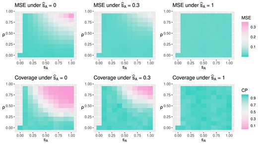
Under true treatment effect being 1.2 at the second time point, the figure displays mean squared error (MSE) and posterior coverage for mixed average treatment effect (ATE) under different simulation truth |$(s_A, \rho )$| and assumed model parameter |$\widehat{s}_A$|⁠. Lower MSE and higher coverage probability (CP) indicate better estimation.

Open in new tabDownload slide

FIGURE 4

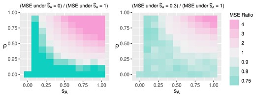
Mean squared error (MSE) ratio under true treatment effect being 1.2 at the second time point.

Open in new tabDownload slide

5 APPLICATION

We apply the proposal to longitudinal clinical data from the Johns Hopkins Scleroderma Center Research Registry. The application examines the subgroup causal effectiveness of MMF initiation regimes among patients who were treated with MMF. Inference is made by sampling and comparing the posterior predictive distribution of counterfactual outcome trajectories across time intervals under different treatment regimes. Disease onset is defined by the emergence of symptoms, which typically occur before and are inquired about during the enrollment visit. The analysis data include patients who enrolled between 2010 and 2020 within 6 years of disease onset. Individual clinical histories before February 28, 2022, with a maximum follow-up of 10 years are used. The data include all available follow-up visits when MMF was never taken and up to 2 years after the first continuous MMF use. At enrollment, 506 scleroderma patients had never been treated with MMF. During follow-up, 194 started MMF. About 80|$\%$| of these individuals are female, 20|$\%$| are African Americans, and 40|$\%$| have diffuse scleroderma, reflecting the overall cohort. Disease onset age has first, second, and third quartiles of 38, 48, and 58 years. Our analysis frames time-varying variables by 6-month intervals because patient visits are expected to be every 6 months. Over 90|$\%$| of MMF initiation occurred within 2.5 years of enrollment.

Assuming tolerance, we examine the first 2 years of MMF use in patients to assess its efficacy over time. If person |$i$| began using MMF at time |$\tilde{s}_i$|⁠, we assess its effectiveness by comparing continuous MMF use to no MMF use over a 2-year period (time intervals |$[\tilde{s}_i, \tilde{s}_i+4)$|⁠). Measurements of modified Rodnan skin score (mRSS) and lung scores, as measured by forced vital capacity (FVC) percent predicted and diffusing capacity for carbon monoxide (DLCO) percent predicted, are considered outcomes in this study. Continuous FVC and DLCO scores are standardized for analysis. The continuous mRSS, assessed in 17 body areas from 0 to 51, was quantilized to the standard normal distribution. Due to clinical data being collected only during clinical visits, biomarker measurements are often missing. For the patients included in the analysis, 82.6|$\%$|⁠, 83.6|$\%$|⁠, and 50|$\%$| had at least 1 interval without FVC, DLCO, or mRSS measurements. Visit patterns may confound the effectiveness of MMF. We define confounders |$M_{it}$| to be indicators of FVC, DLCO, and mRSS updates for person |$i$| at time interval |$t$|⁠, representing visit patterns over time.

Let |$V_i$| be the baseline demographic vector of sex, race, and age. Let |$B_i$| be the baseline status of diffuse scleroderma. Domain knowledge suggests that biomarkers progress upon time since disease onset, denoted as |$S_{it} = t+O_i$|⁠, where |$O_{i}$| is the duration between disease onset and enrollment visit. At time |$t$|⁠, |$\tilde{Y}_{it}$| represents the biomarker measurement carried forward. Because we limit the study to 2 years of continuous MMF use, that is, 4 intervals, dosage information at time |$t$| is summarized by the vector |$D(A_{i,0:t}) = \lbrace \mathbb {1}\big ( \sum ^t_{\ell =1}A_{i\ell }=1\big ),\ldots ,\mathbb {1}\big ( \sum ^t_{\ell =1}A_{i\ell }=4\big )\rbrace$|⁠, where |$A_{i, 0:t} = (A_{i1},\ldots , A_{it})$| is the binary vector of whether person |$i$| was observed to be on MMF over time. In addition, the time between disease onset and MMF initiation is denoted by |$I_{it}$|⁠, which is zero when |$A_{it} = 0$| and |$S_{it^{\prime }}$| when |$A_{it} = 1$|⁠, where |$t^{\prime }$| is the time of treatment initiation, that is, |$A_{i,t^{\prime }-1} = 0$|⁠, |$A_{it^{\prime }} = 1$|⁠, and |$t^{\prime } \le t$|⁠. We assume the following joint model:

where |$\phi _1(\mathcal {H}_{it}) = \lbrace 1, \tilde{Y}_{i,t-1}, V_i, B_i, ns(S_{it},\nu _s), B_i \times ns(S_{it},\nu _s)\rbrace $|⁠, |$\phi _2(\mathcal {H}_{it})\phi _A(\overline{A}_{i,0:t})^T = \lbrace D(\overline{A}_{i,0:t}), V_i\times D(\overline{A}_{i,0:t}),B_i\times D(\overline{A}_{i,0:t}), I_{it}\times D(\overline{A}_{i,0:t})\rbrace$|⁠, |$(b^Y_{i0},b^M_{i0},b^A_{i0})^T\sim N(0,G)$|⁠, and we assume |$\nu _s=4$|⁠. Specifically, |$(b^Y_{i0},b^M_{i0},b^A_{i0})\in \mathbb {R}^7$| and the covariance matrix |$G\in \mathbb {R}^{7\times 7}$| when |$\widehat{s}_A \gt 0$|⁠.

Figure 5 displays model validation results for one-step forward predictions. We use 5-fold cross-validation to test predictive accuracy at each of the 10 time intervals, conditioning on the observed history up to a given time and implementing the prediction procedure as in the causal effect estimation. Black triangles represent the observed mean of time-varying variables at each time. The colored curves and areas represent the posterior mean and 95|$\%$| posterior credible interval of the one-step forward prediction for each time-varying variable, under various posited values of |$b^A_{i0}$|’s standard deviation, |$\widehat{s}_A$|⁠.

FIGURE 5

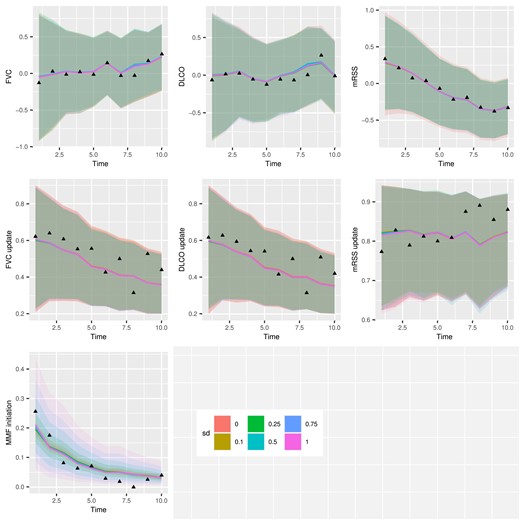
Application one-step forward prediction accuracy plot for each dependent variable in the multivariate generalized linear mixed-effects models (MGLMM).

Open in new tabDownload slide

For person |$i$| with MMF during follow-up, we compare 2 regimes |$q_1$| and |$q_2$| starting at time |$\tilde{s}_i$|⁠, conditional on the clinical history up to time |$\tilde{s}_i-1$|⁠, that is, |$(V_i, \overline{A}_{i,0:(\tilde{s}_i-1)}, \overline{Y}_{i,0:(\tilde{s}_i-1)}, \overline{M}_{i,0:(\tilde{s}_i-1)})$|⁠. For counterfactual trajectories under regime |$q_z$|⁠, |$(\overline{Y}_{i,\tilde{s}_i:(\tilde{s}_i+3)}(q_z),\overline{M}_{i,\tilde{s}_i:(\tilde{s}_i+3)}(q_z))$|⁠, |$z = 1,2$|⁠, we obtain posterior samples |$\lbrace \overline{Y}^{(\ell )}_{i,\tilde{s}_i:(\tilde{s}_i+3)}(q_z), \overline{M}^{(\ell )}_{i,\tilde{s}_i:(\tilde{s}_i+3)}(q_z); \ell = 1,\ldots ,N_{post})\rbrace$| based on Web Appendix C. The comparative effectiveness of the 2 regimes is quantified by the averaged biomarker differences over time, |$\mathbb {D}_j = \lbrace \sum _{i\in T} d^{(\ell )}_{ij} / N_{T}; \ell =1,\ldots ,N_{post}\rbrace$|⁠, where |$j \in \lbrace 0,1,2,3\rbrace$| indexes time since regimen application, |$d^{(\ell )}_{ij} = Y^{(\ell )}_{i,\tilde{s}_i+j}(q_1) - Y^{(\ell )}_{i,\tilde{s}_i+j}(q_2)$|⁠, and |$T$| is the subgroup of interest. Figure 6 summarizes the CMATE of MMF on FVC, DLCO, and mRSS, at 6-month intervals from 0 to 2 years after MMF initiation for diffuse (red) and non-diffuse (blue) patient subgroups. The Y-axis is the difference (population standard deviation units) in each counterfactual biomarker outcome if patients receive treatments that contain MMF versus not. The figure shows the posterior mean (black dot) and 95|$\%$| credible interval (vertical bar) of |$\mathbb {D}_j$| over the 2 years of regimen comparison, that is, |$j=0, 1, 2, 3$|⁠, under posited values of |$\widehat{s}_A\in \lbrace 0, 0.1, 0.25, 0.5, 0.75, 1\rbrace$| indicated by the decrease in opacity as |$\widehat{s}_A$| increases.

FIGURE 6

Application causal estimation by subgroup diffuse versus limited scleroderma. The Y-axis is the difference in the biomarkers (forced vital capacity [FVC], diffusing capacity for carbon monoxide [DLCO], and modified Rodnan skin score [mRSS]) under regimens containing versus not containing mycophenolate mofetil (MMF), projected over 2 years after MMF initiation.

Open in new tabDownload slide

Figure 6 shows that incorporating MMF into the treatment of patients with diffuse scleroderma significantly improves skin score over 2 years, assuming drug tolerance and continuous use. This is consistent with the finding in Scleroderma Lung Study II (Tashkin et al., 2016). The major difference is that we investigated the incorporation of MMF in the treatment of scleroderma patients, whereas the clinical trial compared the use of MMF alone for 24 months versus cyclophosphamide for 12 months followed by a placebo for 12 months. Given that patients may be receiving other therapies, MMF does not improve FVC when averaged within diffuse scleroderma subgroups. Furthermore, adding MMF to the treatment of patients without diffuse scleroderma has no discernible benefit within 2 years of MMF initiation. This has clinical implications because MMF is an immunosuppressive agent that may increase the risk of serious infection and gastrointestinal side effects. We observe that treatment practices for regimens containing or not containing MMF may differ in the real world. Further research is needed to examine the impact of this difference.

6 DISCUSSION

The main contribution is to develop a Bayesian approach to causally estimate the subgroup effectiveness of binary treatment paths on longitudinal outcomes while accounting for time-varying confounders and time-invariant unmeasured confounding. A MGLMM can model biomarker dynamics and treatment assignment simultaneously, allowing for unmeasured confounding. Under correct model specification, our approach will consistently estimate the causal effects of treatment paths even when unmeasured confounding certainly exists or when an unconfounded variable or instrumental variable is unavailable. The proposed MGLMM has a particular representation of unmeasured confounding governed by |$s_A$|⁠, the standard deviation of the treatment assignment random effect, and the correlation |$\rho$| between treatment assignment and biomarker dynamics. A small |$\rho$| and a large |$s_A$|⁠, or a large |$\rho$| and a small |$s_A$| will cause heavy unmeasured confounding. The estimated value of |$\rho$| may inform the presence of unmeasured confounders. The method could potentially be extended to guide the inclusion of other latent variable models in Bayesian causal inference.

The unconfoundedness assumption cannot be tested without guaranteed or controlled treatment assignment randomization. Parametric model assumptions on random effects are not needed for causal inference under the strong assumption of unconfoundedness. However, treating rare chronic diseases in clinics often involves unmeasured confounders. We recognize that there is no free lunch in causal inference, and relaxing the unconfoundedness assumption requires untestable model specification assumptions. The parametric model assumption helps identify treatment effects even when unmeasured confounding may exist. The structure of MGLMM provides insight into how the particular kind of unmeasured confounding impacts the causal effect of treatment paths. Testing the validity of the random effects distributional assumption a posteriori is possible but not standard (McCullagh, 2019), such as by checking residual normality. In the application, the moderate sample size makes the detection of non-Gaussianity in the marginal distribution of multivariate random effects improbable. Exploring the necessity of distributional assumption or expanding to a larger family of multivariate distributions on the MGLMM random effects are important future directions.

The proposed Bayesian GCA uses the MGLMM as the time-evolving generative component and updates to subject-specific random effects over time as patient history accumulates. Our algorithm allows subgroup treatment path evaluation. Furthermore, existing ways to combine PS and outcomes models in Bayesian causal inference include PS-based outcomes distribution, shared parameters or priors, and posterior-based inverse probability weighting or doubly robust estimators (Li et al., 2022). Our method falls under the category of having shared parameters or priors between PS and outcome models, using a dependence structure to connect them through covariances among latent variables. Finally, instead of assuming no unmeasured confounding and conducting post hoc analysis to assess bias due to unobserved confounding, the proposal estimates causal effects conditional on different values of the sensitivity parameter, that is the variance of unobserved treatment assignment heterogeneity specified prior to the model estimation. Our approach reduces to the standard GCA when the sensitivity parameter is zero, indicating no unmeasured confounding. Future extensions of the method include categorical and count outcomes, multiple or continuous treatments, and more flexible distributional assumptions on patient heterogeneities.

A limitation of the proposal is that the current framework is built upon regular time intervals. This was made possible because, in the application setting under consideration, scleroderma is a chronic condition that expects patient visits every 6 months, which are typically driven by physicians. However, as stated in Pullenayegum and Lim (2016), recommended visit intervals may not be followed perfectly. Furthermore, in this case, the deviation from the recommended visit intervals could be attributed to factors that are not recorded in the patient’s charts, such as adverse effects and frailty. The current work summarizes patient visit patterns using time intervals, ignoring the impact of irregular and covariate-driven visit times. It is an important direction for future research to extend the current framework to continuous time and account for irregular visit patterns. Furthermore, the proposal can be naturally extended to account for exogenous time-varying unmeasured confounders when the data have a sufficient number of observations per subject, such as assuming that the random effects are time-varying and Gaussian processes.

ACKNOWLEDGEMENT

We thank Adrianne Woods for excellent database management support, the patients of the Johns Hopkins Scleroderma Center Research Registry for their participation in this foundational resource, and Dr. Joseph Hogan for his knowledgeable comments.

FUNDING

This work was supported in part by the Johns Hopkins inHealth initiative, the Scleroderma Research Foundation, the Nancy and Joachim Bechtle Precision Medicine Fund for Scleroderma, the Manugian Family Scholar, the Donald B. and Dorothy L. Stabler Foundation, the Chresanthe Staurulakis Memorial Fund, the Sara and Alex Othon Research Fund, NIH P30AR070254, and NIH/NIAMS K24AR080217.

CONFLICT OF INTEREST

None declared.

DATA AVAILABILITY

The data that support the findings in this paper are available upon reasonable request from the Johns Hopkins Scleroderma Center Research Registry PI, Dr. Ami Shah ([email protected]).

References