


ABSTRACT
It is of interest to health policy research to estimate the population-averaged longitudinal medical cost trajectory from initial cancer diagnosis to death, and understand how the trajectory curve is affected by patient characteristics. This research question leads to a number of statistical challenges because the longitudinal cost data are often non-normally distributed with skewness, zero-inflation, and heteroscedasticity. The trajectory is nonlinear, and its length and shape depend on survival, which are subject to censoring. Modeling the association between multiple patient characteristics and nonlinear cost trajectory curves of varying lengths should take into consideration parsimony, flexibility, and interpretation. We propose a novel longitudinal varying coefficient single-index model. Multiple patient characteristics are summarized in a single-index, representing a patient's overall propensity for healthcare use. The effects of this index on various segments of the cost trajectory depend on both time and survival, which is flexibly modeled by a bivariate varying coefficient function. The model is estimated by generalized estimating equations with an extended marginal mean structure to accommodate censored survival time as a covariate. We established the pointwise confidence interval of the varying coefficient and a test for the covariate effect. The numerical performance was extensively studied in simulations. We applied the proposed methodology to medical cost data of prostate cancer patients from the Surveillance, Epidemiology, and End Results-Medicare-Linked Database.
1 INTRODUCTION
Longitudinal medical cost data are the healthcare expenditures of each patient during the course of their lifetime. Medical cost data provide important information to policy-makers and health services researchers (Mariotto et al., 2011, 2020). For example, government and insurance companies are often interested in cost projection, that is, forecasting the total healthcare cost or disease-specific cost in the future years. Estimates of population-averaged longitudinal cost trajectory can provide the basis for cost projections. The National Cancer Institute (NCI) developed a cost estimation approach based on descriptive statistics (Mariotto et al., 2011), where longitudinal cancer care costs from the initial diagnosis to death are summarized into three care phases: initial (within 12 months of diagnosis), terminal (within 12 months of death), and continuing care phase (all the months in between). This method does not address the statistical complication due to censoring and ignores the dependence of phase-specific costs on survival, which is highly likely given the common correlation between longitudinal cost and survival data.
In a more statistically rigorous approach, Li et al. (2018) introduced the concept of population-averaged longitudinal medical cost trajectories and developed related estimation approaches. These trajectories are estimated as the expectation of longitudinal costs conditional on survival (henceforth referred to as “cost trajectory”). Here, “conditioning on survival” is crucial. To elaborate, suppose the interest is the average cancer care costs in year 4 after diagnosis. Some patients with costs data in year 4 may have died in year 5, while others died in year 8. For the former, the year 4 costs would likely be high due to its close approximation to terminal care; for the latter group, the costs in year 4 may be low and come from maintenance therapy or surveillance. Hence, the “expectation” of the cost trajectory curves must be taken over patients with similar survival times, to reveal the time-dependent healthcare consumption in an aggregated manner. With the concept of cost trajectories, the use of artificially defined phases, and cutoffs can be avoided.
However, previous research did not study the effects of patient characteristics on cost trajectories. With the emergence of personalized medicine, the number of cancer subtypes and therapy subtypes has increased substantially, resulting in smaller eligible subpopulations. Estimating costs separately within each subpopulation is not feasible when the subpopulations are defined by many patient characteristics, and it is inefficient when comparisons between various patient characteristics are of interest. This paper aims to address these limitations by proposing a parsimonious, flexible, and interpretable regression model to explore the association between baseline covariates and the longitudinal medical cost trajectories. As the trajectories are survival-dependent and subject to censoring, the proposed regression model includes survival time as a covariate.
This research cannot be achieved by using the shared random effects model to jointly model the longitudinal cost data and survival time (Liu et al., 2007; Liu 2009; Chen et al., 2016). These methods are not suitable for our objective, as they formulate the hazard of death as a function of patient characteristics and longitudinal cost data among the at-risk patients. Moreover, shared random effects models may encounter prohibitive computation due to the use of nonlinear longitudinal models for individual-level costs, and non-normality of the cost data. While some research has explored regression models for total cost or cumulative cost up to a specific time point among the at-risk patients at that time, (Lin et al., 1997; Lin, 2003; Bang 2005; Baser et al., 2006; Zhao et al., 2012); these methods cannot be used to study the cost trajectories and their determinants.
Besides tackling a new statistical problem, the proposed methodology is novel in the following aspects. First, the longitudinal medical cost data is modeled without a distributional assumption to handle potentially non-normality in the cost data, including skewness, zero-inflation, and heteroscedasticity. Second, patient characteristics are collapsed into a single-index to represent the propensity of healthcare use, which graphically quantifies the heterogeneous effects given various combinations of patient characteristics. The uncertainty associated with covariates and cost trajectories is properly modeled. Third, the complex relationship between cost trajectory and survival time is modeled by a flexible bivariate-varying coefficient surface. Fourth, we appositely cope with the censored covariate (ie, survival time) to ensure the identifiability of the conditional mean of cost given survival.
To achieve these goals, we propose a semiparametric marginal approach for estimating the longitudinal medical cost trajectory given survival, and conducting inference for the baseline covariates. The potential heterogeneous subgroup effect on the outcome cost trajectory through an unknown function of covariates can be assessed. The proposed method enjoys flexibility while achieving efficiency by utilizing cost data from both uncensored and censored patients through a novel extended generalized estimating equation (GEE) approach. This approach is motivated by the varying-coefficient model considered in Wu et al. (2019) for risk assessment with multiple covariates, which can handle large amounts of temporal data and baseline covariates. To use all the covariates effectively, our single-index term focuses on a weighted linear combination of all covariates as a summary risk score. We model the cost trajectory curve as a function of this summary risk score, the measurement time, and survival with possible interaction terms. The coefficients (or weights) in the single-index term measure the effect of the covariate for the change of the outcomes. An iterative estimation procedure is developed for the proposed model. We construct pointwise confidence intervals for the cost trajectory curves. Based on the inference procedure, we can identify the important characteristics and the associated subgroup of patients that has different mean costs in different time periods, and the global relationships between the costs and baseline covariates.
The rest of this paper is organized into 5 sections. We introduce the model notation in Section 2. Estimation and inference procedures are given in Section 3. Numerical results on a real-world data example and simulation data are presented in Sections 4 and 5, respectively. Additional technical details, model-checking results and simulations are presented in the Web Appendix.
2 MODEL
We observe independent and identically distributed data from n subjects, |$\big \lbrace \boldsymbol{Y} _i, \boldsymbol{X} _i,T_i=\min (\widetilde{T}_i,C_i),\delta _i = 1\lbrace \widetilde{T}_i\le C_i);i=1,\ldots,n\big \rbrace$|. |$\boldsymbol{X} _i$| is the patient’s baseline variable of length p. |$\widetilde{T}_i$| is the time to the terminal event of interest. Ci is the time to censoring. δi is the event indicator: δi = 1 if the terminal event occurs prior to censoring. τ can be the maximum observed event time (ie, max {Ti|δi = 1}, i = 1|$,\ldots,$|n) or alternatively a prespecified cutoff time of interest, such as ten years in the motivating case study. |$\boldsymbol{t} _i = (t_{i1},t_{i2}, ..., t_{in_i})^T$| is the measurement time and ni is the number of longitudinal measurements. |$\boldsymbol{Y} _i = (Y_{i1},Y_{i2}, \ldots, Y_{in_i})^T$| is a vector of longitudinal outcome up to observed survival time Ti, j = 1|$,\ldots, $|ni. For notation convenience, we write Yij = Yi(tij). We assume that Ci and |$(\widetilde{T}_i,Y_{ij})$| are independent given covariates |$\boldsymbol{X} _i$|.
A simple extension of the cost trajectory estimation methods (Li et al., 2018; Wang et al., 2020) by incorporating covariates is to assume that the covariates have linearly additive effects:
In this partially linear model, |$\mu _{01}(t,\widetilde{T})$| is a flexible bivariate function of a baseline trajectory surface (eg, the surface corresponding to zero covariate values). Each of the p covariates has a constant coefficient, denoted by |$\boldsymbol{\theta }_1=(\theta _{11},...,\theta _{1p})^T$|. g(·) is the link function. Although this model has a simple form, it assumes that every covariate is associated with a constant shift on the entire cost trajectory, regardless of the time t and trajectory length |$\widetilde{T}$|. This is a very restrictive assumption and it often does not hold. A flexible formulation to remove this restriction is to allow each covariate to have a time-varying coefficient:
But this model is excessively complicated in both estimation and interpretation. To balance both flexibility and parsimony, we combine the ideas from two areas of statistical research, single index models (Wang et al., 2010) and varying coefficient models (Fan and Zhang, 2008), and propose the following longitudinal varying coefficient single-index model:
In this model, we rescale the covariate effect by |$\mu _{11}(t,\widetilde{T})$|, a bivariate varying coefficient function of measurement time and survival. We refer to |$S_i = \boldsymbol{X} _i^T \boldsymbol{\theta }_1$| as the index variable, which collapses all baseline covariates into a single score. This score can be interpreted as the overall propensity of healthcare utilization. Prespecified nonlinear transformation of |$\boldsymbol{X}$| can be used in this single index to enhance flexibility. Here are two additional remarks on the model interpretation:
The baseline bivariate function |$\mu _{01}(t,\widetilde{T})$| can be considered as the “intercept”, which represents the mean reference cost trajectory. It corresponds to the trajectory when all covariates equal to zero, as is the case when covariates are centered before analysis. The covariate effect, or the slope, of the index variable S is |$\mu _{11}(t,\widetilde{T})$|, which quantifies the amount of change in the outcome for each unit of increase in S. The change varies with t and |$\widetilde{T}$|, allowing different parts of the trajectory curves to be bent and twisted differently. This feature is essential for modeling cost trajectories. Initial and terminal care is usually more expensive than continuing care. Therefore a constant slope of S that does not depend on t and |$\widetilde{T}$| is unjustified.
To improve the interpretation of single-index parameter |$\boldsymbol{\theta }_1$|, we consider two standardizations. First, we normalize the categorical baseline covariates by dummy variables (ie, coded as 0 or 1). We further standardize every continuous baseline covariate with mean 0 and variance 1. The effect of the index variable S is |$\mu _{11}(t,\widetilde{T})$|. The weights of individual covariates in the index, |$\boldsymbol{\theta }_1$|, serve as scaling factors, which may enlarge, shrink, or reverse the direction of individual covariate effects in comparison with the effect of the index variable. The amount of scaling is always constrained to have |$\Vert \boldsymbol{\theta }_1 \Vert = 1$| (see Section 3). In the special case when |$\mu _{11}(t,\widetilde{T}) \equiv 0$|, the scaling does not result in any nonzero covariate effect on the outcome, even though some values of |$\boldsymbol{\theta }_1$| takes nonzero values due to the constraint |$\Vert \boldsymbol{\theta }_1 \Vert = 1$|. When |$\mu _{11}(t,\widetilde{T}) \ne 0$|, the elements in |$\boldsymbol{\theta }_1$| measures the magnitude of the individual covariate effects relative to each other.
Since, the covariate |$\widetilde{T}_i$| in model (3) is subject to right-censoring, it is necessary to model the conditional distribution |$F_{\widetilde{T}}(s|T, \boldsymbol{X} )$| of its residual distribution. For illustration purpose, we use the proportional hazards model, though any other survival regression model with time-independent covariates could be used:
For convenience in joint estimation with longitudinal data, we model the log baseline hazard log h0(s) by a penalized spline (Kauermann 2005). Denote the parameters in the baseline hazard as |$\boldsymbol{\beta }_0$|. Then |$\boldsymbol{\beta }= ( \boldsymbol{\beta }_{0}^T, \boldsymbol{\beta }_1^T)^T$| is the parameter vector in model (4).
If the support of |$\widetilde{T}$| lies outside the support of C, |$\widetilde{T}$| is nonidentifiable at (τ, ∞) without further assumptions. In practice, the limited follow-up of a study and/or longer life expectancy for some individuals could result in a significant proportion of subjects to be censored at the maximum follow-up time (τ). For convenience, we call subjects who survived beyond τ long-term survivors (LTS). Since their terminal event is nonidentifiable, our proposed method involves two parts of coefficient weights for the additive unknown functions for LTS and non-LTS; details are discussed in Section 3.
Therefore, we further specify a longitudinal varying coefficient single-index model for subjects with |$\widetilde{T} \gt \tau$|, that is LTS:
This model is similar to (3) but the varying coefficients do not depend on |$\widetilde{T}$|. It describes how the covariates affect the shape of a particular cost trajectory, that of subjects with |$\widetilde{T} \gt \tau$|, through the single index variable. Clearly, the index parameter vectors |$\boldsymbol{\theta }=( \boldsymbol{\theta }_1^T, \boldsymbol{\theta }_2^T)^T$| are not identifiable without further scale restrictions. Without loss of generality, we let |$\boldsymbol{\theta }$| belong to the parameter space |$\boldsymbol{\Theta }=\lbrace \boldsymbol{\theta }_k: \Vert \boldsymbol{\theta }_k\Vert =1,\theta _{k1}\gt 0, \boldsymbol{\theta }_k\in R^p,k=1,2\rbrace$|, where ‖ · ‖ denotes the l2 norm of a vector. In other words, |$\boldsymbol{\theta }$| is standardized to have unit norm. Under this restriction, |$\boldsymbol{\theta }$| in model (3) and (5) are identifiable if μ’s are modeled using spline approximation, which we will discuss in Section 3. To further ensure the model identifiability, we eliminate the first component in |$\boldsymbol{\theta }_k$| (k = 1, 2), the resulting parameter space is denoted by |$\boldsymbol{\Theta }_{-1}=\lbrace \boldsymbol{\theta }_{k,-1}=(\theta _{k2},...,\theta _{kp})^T: \sum _{j\gt 1}\theta _{kj}^2\lt 1,k=1,2\rbrace$|, and |$\theta _{k1}=\sqrt{1-\sum _{j\gt 1}\theta _{kj}^2}$|.
3 ESTIMATION
We first present a simple estimator by using data from subjects who experienced the terminal event prior to τ and subjects who were censored at τ. Then we propose a novel extension of the GEE approach that fully uses data, including subjects who were censored prior to τ. Next, we incorporate variance-covariance modeling to GEE to account for heteroscedasticity in the data. Lastly, we provide remarks on hypothesis testing on the coefficients. Additional technical issues in the model fitting, including selection of knots and smoothing parameters, survival distribution estimation are discussed in Web Appendix.
3.1 No right-censoring prior to maximum follow-up time
We start with estimation without using data from subjects who were censored prior to τ. Consider the 2-part estimating equations for the medical cost trajectory from patient i as
where |$\boldsymbol{V} _i$| is the working covariance matrix that may be misspecified. The functions |$\mu _{01}(\cdot ,\cdot ), \mu _{11}(\cdot ,\cdot ), \mu _{02}(\cdot ),\mu _{12}(\cdot ),\mu _{02}(\cdot )$| in equations (3) and (5) are unspecified and can be approximated using spline functions with truncated polynomial basis. Since the measurement time cannot exceed the survival time, the bivariate cost trajectory function μ01(·,·), μ11(·,·) is defined on an upper triangular area |$(0\lt t\le \widetilde{T})$|. Following Li et al. (2018), we exploit a shrinkage-expansion transformation to define |$\mu _{k1}(t,s)=\overline{\mu _{k1}}(u=t(\tau /s),s),0\lt t\le s$|. The expanded surface |$\overline{\mu _{k1}}(u,s)$| is defined on the rectangular area u, s ∈ (0, τ], where conventional polynomial splines for a bivariate surface are defined. As a result, the nonparametric functions can be approximated well by spline functions such that |$\mu _{k1}(t,s) \approx \boldsymbol{B} _{\mu _{k1}}(t,s) \boldsymbol{\gamma }_{k1},k=0,1$|, where |$\boldsymbol{B} _{\mu _{k1}}(t,s)$| is a vector of bivariate truncated polynomial basis. Each basis function consists of elements of the outer product matrix of vector Bt(t) and Bs(s) with prespecified internal knots on the scale of t and s, respectively. Similarly, for LTS the univariate cost trajectory function |$\mu _{k2}(t) \approx \boldsymbol{B} _{\mu _{k2}}(t) \boldsymbol{\gamma }_{k2},k=0,1$|, where |$\boldsymbol{B} _{\mu _{k2}}(t)$| is a vector of truncated polynomial basis with some prespecified internal knots. Denote the unknown index weight parameters by |$\boldsymbol{\theta }=( \boldsymbol{\theta }_1^T, \boldsymbol{\theta }_2^T)^T$|. Let the spline coefficients |$\boldsymbol{\gamma }=( \boldsymbol{\gamma }_1^T, \boldsymbol{\gamma }_2^T)^T$| where |$\boldsymbol{\gamma }_1=( \boldsymbol{\gamma }_{01}^T, \boldsymbol{\gamma }_{11}^T)^T$| and |$\boldsymbol{\gamma }_2=( \boldsymbol{\gamma }_{02}^T, \boldsymbol{\gamma }_{12}^T)^T$|. The estimates of |$\boldsymbol{\theta }$| and |$\boldsymbol{\gamma }$| are the solutions of the estimating equation for models 3 and 5 corresponding to the model (6), where the jth element of |$E\lbrace \boldsymbol{Y} _i|T_i,\delta _i, \boldsymbol{X} _i\rbrace =: \boldsymbol{\eta }_i$| is approximated by
and |$\boldsymbol{B} _1(t,s,z)= \left( \boldsymbol{B} _{\mu _{01}}(t,s),z \boldsymbol{B} _{\mu _{11}}(t,s)\right)$| and |$\boldsymbol{B} _2(t,z)= \left( \boldsymbol{B} _{\mu _{02}}(t),z \boldsymbol{B} _{\mu _{12}}(t)\right)$|. To overcome the roughness in the trajectory functions, we exploit parameter regularization and specify the penalty function by |$J_{\lambda }( \boldsymbol{\gamma })$|, where the tuning parameter λ controls the level of the roughness in |$\boldsymbol{\gamma }$|. An iterative algorithm is presented in Web Appendix Section 1.1.
Repeatedly solving Web Appendix equations (1) and (3) until convergence leads to the estimator from patients with “partial data”, which is the complete cost data and death time, denoted by |$\widetilde{ \boldsymbol{\gamma }}$| and |$\widetilde{ \boldsymbol{\theta }}$|. The corresponding sandwich covariance estimator for |$\widetilde{ \boldsymbol{\gamma }},\widetilde{ \boldsymbol{\theta }_{-1}}$| is |$\widetilde{ \boldsymbol{\Sigma }}_{-1}= \boldsymbol{H} _{n,\lambda }^{-1} \boldsymbol{M} _n \boldsymbol{H} _{n,\lambda }^{-1}$|, where |$\boldsymbol{M} _n=\sum _{i=1}^n \boldsymbol{D} _{i}^T \boldsymbol{V} _i^{-1}\lbrace \boldsymbol{Y} _i- \boldsymbol{\eta }_i\rbrace \lbrace \boldsymbol{Y} _i- \boldsymbol{\eta }_i\rbrace ^T \boldsymbol{V} _i^{-1} \boldsymbol{D} _{i}$| denotes the variance of the estimating equations, |$\boldsymbol{H} _{n,\lambda }=\sum _{i=1}^n \boldsymbol{D} _{i}^T \boldsymbol{V} _i^{-1} \boldsymbol{D} _{i}+ J_{\lambda }( \boldsymbol{\theta })$| is the Hessian matrix, and |$\boldsymbol{D} _{i}$| is the corresponding design matrix combining |$\boldsymbol{D} _{ \boldsymbol{\theta }i}$| and |$\boldsymbol{D} _{ \boldsymbol{\gamma }i}$|. From delta method, the sandwich covariance estimator for |$\widetilde{ \boldsymbol{\theta }},\widetilde{ \boldsymbol{\gamma }}$| is |$\widetilde{ \boldsymbol{\Sigma }}=\Delta \widetilde{ \boldsymbol{\Sigma }}_{-1} \Delta ^T$|, where |$\Delta =\mathrm{diag}\lbrace J( \boldsymbol{\theta }_1),J( \boldsymbol{\theta }_2), \boldsymbol{I} _{ \boldsymbol{\gamma }}\rbrace$| and |$\boldsymbol{I} _{x}$| is an identity matrix whose dimension is the length of |$\boldsymbol{x}$|.
3.2 Include data with right-censoring prior to maximum follow-up time
To improve estimate efficiency, one wants to use all observed data including those death times that are censored prior to τ. We consider the following extended mean and covariance functions:
We re-define notation |$E\lbrace \boldsymbol{Y} _i\rbrace =: \boldsymbol{\eta }_i^{\prime }$| for this subsection. The iterative algorithm in Section 3.1 can be modified as shown in Web Appendix Section 1.2.
Solving Web Appendix equations (4) and (5) iteratively until convergence leads to the estimator from “all data”, denoted by |$\widehat{ \boldsymbol{\gamma }}$| and |$\widehat{ \boldsymbol{\theta }}$|. To adjust for the variation associated with the survival estimation, the joint sandwich covariance formula for |$\widehat{ \boldsymbol{\beta }},\widehat{ \boldsymbol{\gamma }},\widehat{ \boldsymbol{\theta }}_{-1}$| is |$\boldsymbol{\mathcal {H}} _{n,\lambda }^{-1} \boldsymbol{\mathcal {M}} _n \boldsymbol{\mathcal {H}} _{n,\lambda }^{-1}$|, where |$\boldsymbol{\mathcal {M}} _n$| denotes the corresponding variance of the joint estimating equations, and |$\boldsymbol{\mathcal {H}} _{n,\lambda }$| denotes the joint Hessian matrix. Specifically,
where |$\boldsymbol{\mathcal {S}} _i( \boldsymbol{\beta })$| is the score function for the survival model parameter |$\boldsymbol{\beta }$|, and |$\boldsymbol{\mathcal {D}} _{i}$| is the corresponding design matrix combining |$\boldsymbol{\mathcal {D}} _{ \boldsymbol{\theta }i}$| and |$\boldsymbol{\mathcal {D}} _{ \boldsymbol{\gamma }i}$|.
from the delta method, the sandwich covariance estimator for |$\widehat{ \boldsymbol{\beta }},\widehat{ \boldsymbol{\gamma }},\widehat{ \boldsymbol{\theta }}$| is |$\widehat{ \boldsymbol{\Sigma }}= \boldsymbol{\Delta }\widehat{ \boldsymbol{\Sigma }}_{-1} \boldsymbol{\Delta }^T$| where |$\boldsymbol{\Delta }=\mathrm{diag}\lbrace \boldsymbol{I} _{ \boldsymbol{\beta }},\Delta \rbrace$|. The sandwich covariance estimators for baseline |$\widehat{\mu }_{01}(\cdot ,\cdot ),\widehat{\mu }_{02}(\cdot )$| are thus given by
where |$\widehat{ \boldsymbol{\Sigma }}_{ \boldsymbol{\gamma }_{0l}}$| is the subset of |$\widehat{ \boldsymbol{\Sigma }}$| corresponding to |$\boldsymbol{\gamma }_{0l},l=1,2$|. The variance estimator has a robustness property similar to the parametric sandwich estimator, that is the consistency holds even if the covariance matrix is misspecified. The maximum efficiency will be achieved if the covariance matrix is correctly specified. The sandwich variance estimator can properly account for the variability of estimated survival distribution. When the sample size is relatively small, ignoring the uncertainty from the estimated survival distribution underestimates the variance estimate. An algorithm for implementing the proposed method through an iterative alternating optimization procedure is described in Algorithm 1.

3.3 Hypothesis tests
Applying the estimation procedure described in the previous section, we propose two hypothesis tests for the trajectory curves and covariate index parameters, respectively. In practice, parsimonious models for the varying coefficient are always desirable to reduce computation burden and ease interpretation. To test whether the function μ11(·,·) has a specific parametric form, we set up the hypothesis testing as |$H_0:\mu _{11}(\cdot ,\cdot )=\mu _{ \boldsymbol{\gamma }}(\cdot ,\cdot )$| vs. |$H_a:\mu _{11}(\cdot ,\cdot )\ne \mu _{ \boldsymbol{\gamma }}(\cdot ,\cdot )$| where |$\mu _{ \boldsymbol{\gamma }}(\cdot ,\cdot )$| could be a given parametric function with parameter vector |$\boldsymbol{\gamma }$|. For example, we can test whether there exists nonconstant trajectory effects on the covariate index by setting |$\mu _{ \boldsymbol{\gamma }}(t,s)=\gamma _0$|; or we can test whether there exists linear interaction effects between t and covariate(s) by setting |$\mu _{ \boldsymbol{\gamma }}(t,s)=\gamma _0+\gamma _1 t$| (a linear function), where we assume γ0 and γ1 are some unknown constants. We introduce a Wald statistic to test whether the complex varying coefficient on the covariate index can be replaced by a simpler nested parametric function as aforementioned. The Wald test is defined by testing whether multiple spline parameters equal zero,
where R is the index matrix that corresponds to the spline parameters. Following the results in Yu and Ruppert (2002); Bai et al. (2009), Tn asymptotically follows a chi-square distribution with degrees of freedom equal to the difference in the number of parameters between the null and alternative.
Given that the trajectory effect for the covariate index is not zero, μ11(·,·) ≠ 0, we can also test whether the individual covariate effect θkl (k = 1, 2; l = 2|$,\ldots,$|p) equals to zero. This test is based on the asymptotic distribution |$\widehat{\theta }_{kl} / \sigma _{\theta _{kl}}\rightarrow _d N(0,1)$| under H0.
4 APPLICATION TO SEER-MEDICARE
Prostate cancer is the most common cancer and the second leading cause of cancer death among men in the United States (Cronin et al., 2018), with 3.1 million new cases of prostate cancer diagnosed between 2003 and 2017 (Siegel et al., 2020). It is slow-growing cancer that primarily affects elderly men, causing symptoms such as pain, fatigue, and difficulty urinating, which significantly impact patients’ quality of life. Prostate cancer is also one of the most expensive healthcare problems in the United States, with an estimated economic burden of around 20 billion US dollars in 2020 (Mariotto et al., 2020). Both the survival and economic burden of prostate cancer continue to increase, and the differences in longitudinal cost trajectory by patient characteristics could inform public health planning related to survivorship and care.
We apply the proposed method to the medical cost data of patients with local/regional prostate cancer from the Surveillance, Epidemiology, and End Results (SEER)-Medicare linked database. The SEER program is a population-based cancer registry that covers approximately 35% of the US population across 17 SEER areas, while the Medicare program provides insurance coverage to 97% of Americans aged 65 years and older. The SEER data can be licensed through the National Cancer Institute upon approval of study protocols. The study cohort consisted of 161 630 patients aged 65 years or older, who were diagnosed with prostate cancer between January 1, 2003 and December 31, 2015. Medical costs included Medicare payments for inpatient and outpatient services covered by Medicare Parts A and B from the month of diagnosis until death or the end of follow-up (ie, December 31, 2016). To ensure the completeness of claims data within the first year of cancer diagnosis and to determine the treatment received during this period, we further restricted the study cohort to patients with continuous Parts A and B enrollment and who were not enrolled in Health Maintenance Organization (HMO)s in this duration. The goal was to analyze the effect of patient baseline characteristics and the status of the definitive treatment (ie, surgical or radiation) within the first year of diagnosis on the population-averaged medical cost trajectory.
In our analysis, the response Y is a right-skewed and zero-inflated continuous outcome on the original dollar scale. We specified a compound symmetry structure to accommodate the within-subject correlation of the longitudinal cost. The explanatory variables included comorbidity scores, age at diagnosis, race/ethnicity, and receipt of definitive treatment within 12 months after initial diagnosis (ie, radiotherapy (yes/no) or surgery (yes/no)). We dichotomized the age at diagnosis (65–74 vs. ≥ 75). Patients’ modified Charlson comorbidity scores were calculated using Medicare claims from inpatient, outpatient, and physician professional services within the 12 months before the month of cancer diagnosis, and the comorbidity score was dichotomized (0–1 vs. >1) (Klabunde et al., 2000, 2007). Race/ethnicity was classified into three categories: non-Hispanic White, non-Hispanic Black, and others (including Hispanics and non-Hispanic other races). For model fitting, we used a truncated quadratic spline basis with 5 equally spaced knots in both the mean functions of costs and the hazard function of survival. To select the optimal model, we employed the proposed Wald statistic and found that, at a 1% significance level, the varying coefficient effect for the covariate index was not zero, indicating that the varying coefficients μ11(t, s) and μ12(t, s) were nonlinear. We selected the optimal penalty parameter via the quasi-generalized cross-validation (QGCV) criterion and applied the convergence criterion, which required the maximum absolute difference between the current and previous parameter estimate to be less than 10−4. Finally, we computed the corresponding pointwise confidence intervals for the mean baseline cost trajectory.
The reference group represents non-Hispanic White patients aged 65–74 who had comorbidity scores of 0–1 and did not receive radiotherapy or surgery within 12 months of cancer diagnosis.
4.1 Cohort characteristics
We stratified patients at the survival year of 10 (40 quarters), and the mean age for the non-LTS group was 73.2 years, while for the LTS group, it was 71.8 years. Table 1 shows that among patients who survived over 40 quarters, a high proportion of patients (80.7%) had a comorbidity score of 0–1, compared to patients who survived below 40 quarters (67.2%). Additionally, the LTS group had a higher proportion of non-Hispanic White patients (79.8%) and a lower proportion of non-Hispanic Black patients (8.7%). The LTS group also had a lower proportion of patients aged over 75 years (28.0%), and a higher rate of radiotherapy or surgery as initial treatment within 12 months after cancer diagnosis.
Summary statistics (count and percent) and estimation results (point estimate and 95% CI) of linear coefficients for medical cost trajectory from SEER-Medicare prostate cancer data.
| Count | Percent | Estimate | 95% CI | |
|---|---|---|---|---|
| Time to death ≤40 quarters (N = 134 163) | ||||
| Comorbidity score | ||||
| 0–1 | 90 130 | 67.2 | – | – |
| >1 | 44 033 | 32.8 | 0.632 | [0.613, 0.651] |
| Age at baseline | ||||
| 65–74 | 84 969 | 63.3 | – | – |
| ≥75 | 49 194 | 36.7 | −0.336 | [−0.360, −0.313] |
| Race | ||||
| Non-Hispanic White | 101 810 | 75.9 | – | – |
| Non-Hispanic Black | 15 466 | 11.5 | 0.266 | [0.231, 0.302] |
| Others | 16 887 | 12.6 | 0.135 | [0.097, 0.173] |
| Initial treatment within 12 months after cancer diagnosis | ||||
| Radiotherapy | 57 474 | 42.8 | 0.629 | [0.608, 0.649] |
| Surgery | 38 964 | 29.0 | 0.051 | [0.025, 0.078] |
| Time to death >40 quarters (N = 27 467) | ||||
| Comorbidity score | ||||
| 0–1 | 22 162 | 80.7 | – | – |
| >1 | 5305 | 19.3 | 0.994 | [0.991, 0.997] |
| Age at baseline | ||||
| 65–74 | 19 768 | 72.0 | – | – |
| ≥75 | 7699 | 28.0 | 0.013 | [−0.015, 0.041] |
| Race | ||||
| Non-Hispanic White | 21 928 | 79.8 | – | – |
| Non-Hispanic Black | 2400 | 8.7 | −0.055 | [−0.088, −0.022] |
| Others | 3139 | 11.5 | −0.038 | [−0.067, −0.009] |
| Initial treatment within 12 months after cancer diagnosis | ||||
| Radiotherapy | 14 499 | 52.8 | 0.075 | [0.053, 0.097] |
| Surgery | 8975 | 32.7 | −0.042 | [−0.063, −0.021] |
4.2 Nomogram on total cost summary
Since the estimated linear coefficients of |$\boldsymbol{\theta }$| (Table 1) lacked direct interpretation as a covariate effect in a regression model, we applied the concept of nomograms to place |$\boldsymbol{\theta }$| in the context of covariate effect on costs. Specifically, Figure 1 shows the use of a nomogram to summarize the covariate effect through distinct index points on total cost given survival time. A nomogram is widely used as a visualization tool to depict the relationship between covariates and outcomes for complex statistical models such as the Cox proportional hazards model and logistic regression model. In the past 2 decades, nomograms have been widely used in clinical decision-making for prostate cancer patients, such as the assessment of time-to-PSA level elevation recurrence (Kattan, 2003), and the Partin Table for pathological cancer stage (Partin et al., 1993). As illustrated in Figure 1, patients in the reference group have 0 total points, on average they costed $144K, $167K, or $182K, if they died at 16, 24, or 32 quarters after the cancer diagnosis, respectively. Given other conditions unchanged, a similar non-Hispanic Black patient has 0.266 total points, and the mean total cost was $161K, $186K, or $203K, respectively, which is higher than their non-Hispanic White counterparts. If the patient received radiotherapy in initial treatment and had over 1 comorbidity score, the total points become 0.895, and the average total costs reach $199K, $230K, or $254K, respectively. Comparatively, the mean total cost for LTS in the reference group is $106K. Fixing other conditions, the total points value for a similar non-Hispanic Black is −0.055, and thus that patient costed $2K less on average for LTS. Note that the area under the curve of cost trajectory is the mean total cost reported in the nomogram. Receiving radiotherapy in initial treatment barely changed the total cost for LTS, while a high comorbidity score is associated with a $43K increase in total cost. The use of nomograms allowed us to translate a complicated single-index regression model into informative graphical presentations that are easier to comprehend for a lay audience and policymakers on cost estimation and evaluation.
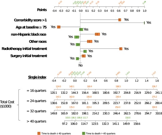
SEER-Medicare data application results of the cost nomogram. Instructions for policymakers are as follows: first, locate the patient’s baseline covariates on the top axes, and draw a vertical line straight upwards to the points axis to determine how many points are contributed. Second, sum the points achieved for each covariate and locate this sum on the single index axis below. Third, draw a vertical line straight down to find the patient’s total cost ($1000), assuming the time to death is 16, 24, 32, or over 40 quarters. The total cost of LTS is limited to be within 40 quarters. Green: time to death ≤ 40 quarters; orange: time to death > 40 quarters.
4.3 Varying coefficient and linear index associated with cost
Figure 2 clearly shows that the index values were positively associated with cost trajectory, and the relations were not linear. This evidence aligns with the hypothesis test result (H0: μ1k(t, s) is constant, k=1, 2; P-value <0.0001) suggesting that a simple model such as (1) is inadequate to capture the complex relationship between covariates and cost trajectory. Figure 2 suggests a dramatic elevation of the cost trajectory right after the cancer diagnosis, especially for subjects who received radiotherapy within the first year of diagnosis. We can find that among patients who died 16 quarters after the cancer diagnosis, the first quarter costs were highest for non-Hispanic Black ($9292; $8985–$9599), lower for non-Hispanic White ($7446; $7117–$7775), and intermediate for others ($8,383; $8074–$8692). After 1 year of diagnosis, the costs went down gradually, and the trajectories for different indexes seem to overlap in the continuing care phase. Within 1 year before death, the cost trajectory quickly increases, and the rates of cost increase are generally higher for higher index values. For example, for a non-Hispanic Black patient aged 65–74 who had comorbidity scores greater than 1 and received radiotherapy as initial treatment, the corresponding single index value was 1.014 and the mean total cost was $150K.
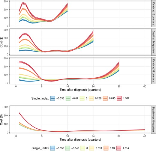
SEER-Medicare data application results of the cost trajectories under different indexes when survival time is 16, 24, 32, or over 40 quarters. A single index equals 0 as a reference group. For patients who died within 40 quarters after cancer diagnosis (or for LTS), the single index is −0.336 (0.013) for patients aged over 75, 0.266 (-0.055) for non-Hispanic Black, −0.07 (−0.042) for patients aged over 75, non-Hispanic Black, 0.895 (0.13) for non-Hispanic Black with receipt of radiotherapy as an initial treatment, 1.527 (1.014) for non-Hispanic Black who has an over 1 comorbidity score and receipt of radiotherapy as an initial treatment. The unmentioned conditions are the same as the reference group. For time to death ≤ 40 quarters, single-index = −0.336 (blue), −0.07 (green), 0 (lime), 0.266 (yellow), 0.895 (orange), and 1.527 (red); for time to death > 40 quarters, single-index = −0.055 (blue), −0.042 (green), 0 (lime), 0.013 (yellow), 0.13 (orange), and 1.014 (red).
In Table 1, among patients who survived below 40 quarters, we observed a higher mean cost trajectory for patients who had higher comorbidity scores, were between 65 and 74 years of age, non-Hispanic Black, and received radiotherapy or surgery as the initial treatment. This result is consistent with findings published in Schmid et al. (2016) and Trogdon et al. (2019). Since all covariates in our regression model are binary, and the linear coefficients are on a unit circle, we are able to compare the relative effects of the covariates. For example, in Table 1, the mean effect of being non-Hispanic Black (0.266; 0.231–0.302) is twice as large as being in “other” race categories (0.135; 0.097–0.173). Table 1 also shows some interesting findings for patients who survived over 40 quarters (LTS). We observed slightly lower costs for patients who were non-Hispanic Black or other races and who received surgery within the first 12 months of a cancer diagnosis. The significantly positive coefficients associated with non-Hispanic Blacks and other races compared to non-Hispanic Whites suggest that policymakers should explore factors that can potentially contribute to the higher cost of racial/ethnic minority patients for Medicare.
4.4 Reference cancer care cost
Putting together all the reference trajectories at different survival quarters s = 1, 2|$,\ldots,$| we can depict a visually “smooth” bivariate surface as shown in Figure 3b. Since the measurement time t = 1, 2|$,\ldots,$|s, the surface is on a triangular region. The reference medical cost trajectory has a nonlinear dependence on the time after diagnosis, and the corresponding relationships are highly heterogeneous for different survival times. Fixing the time to death, the trajectories are rough “U-shaped”, which means that patients are likely to receive more care right after the initial cancer diagnosis, as well as more intensive care towards the end of life (EOL).
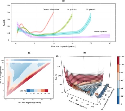
SEER-Medicare data application results for the estimated reference cost trajectories (a) 2D heatmaps and (b) 3D “surface” with 95% confidence intervals with 95% upper and lower bounds in gray meshes.
In Figure 3a, we first look “upward” (bottom to top) at the trajectory surface within 1 year after diagnosis, the costs are lower for patients who survived longer. The treatment guideline for prostate cancer published by the American Urological Association (AUA) makes treatment recommendations based on a risk assessment that incorporates factors such as cancer stage, serum prostate-specific antigen, cancer grade, and tumor volume on biopsy (Eastham et al., 2022). Patients who survived longer are likely those who were healthier and had a lower risk of cancer progression; thus were suitable candidates for observation or active surveillance, which was less expensive than definitive treatment options (eg, surgical or radiotherapy). The boundary oscillation close to τ may be due to limited sample size and spline approximation. Looking “backward” (right to left) at the trajectory pattern from the time to death, there is a change point around four quarters before death, which aligns with the definition of terminal phase in NCI's cost reporting (Mariotto et al., 2020). In Figure 3a, higher terminal care cost is a common pattern for the elderly due to the use of all services in EOL care, including hospitalization related and unrelated to cancer, hospice care, and outpatient services (ie, office or emergency room visits and hospital outpatient procedures) (Duncan et al., 2019). However, the trajectory is L-shaped on average among LTS, possibly because the observed costs are not all from their EOL care.
Besides the cost within the first few months after diagnosis and the last few months before death, in the middle of a lifespan, we observe that patients with longer-term survival have lower average quarterly costs. For example, the cost at the 8th, 12th, 16th, and 12th quarters postdiagnosis for patients who died at 16, 24, 32, and over 40 quarters follows a decreasing trend: $5888, $4007, $3864, and $3787, respectively. However, the cumulative cost in the middle of patients’ lifespans may be higher for patients who survive longer.
The complex nonlinear interdependencies are clearly seen between time after diagnosis, time to death, and costs. In addition, the estimated compound symmetry correlation for patients who survived within 40 quarters after diagnosis is 0.07, which suggests a low positive within-subject correlation in costs. The corresponding correlations are slightly lower for LTS (0.05) because LTS includes subjects with different survival times and the variability of costs is thus larger.
5 SIMULATION STUDY
In this section, we study the finite sample performance of the proposed method by two simulation examples:
The outcome Y is sampled from a normal distribution with baseline mean trajectory μ01(t, s) = cos(2πt/s) + 1 to mimic U-shaped trajectories for the non-LTS subjects (0 < s ≤ τ), and μ02(t) = cos(2πt) × 1(t ≤ 0.5) − 1(t > 0.5) + 1 to mimic the L-shaped trajectories for LTS (s > τ). The variance is 0.25 with a compound symmetry correlation structure and the correlation is 0.2.
The outcome Y is sampled from a gamma distribution with chosen shape and scale parameters such that the baseline mean trajectory follows μ01(t, s) = exp(t/s) to mimic increasing trajectories for the non-LTS subjects (0 < s ≤ τ), and μ02(t) = exp(t) for LTS (s > τ). The variance depends on mean as var(Y) = μ2. To simulate zero-inflation, the outcome Y is multiplied by 10/9, and then 10% outcome values are randomly set to 0.
For both examples, the covariates X = [X1, X2] are independently generated from Uniform[0,1] and Bernoulli(0.5). The mean index functions |$\boldsymbol{X} ^T \boldsymbol{\theta }_{1}= \boldsymbol{X} ^T \boldsymbol{\theta }_{2}=(X_1+X_2)/\sqrt{2}$|, and the varying coefficient μ11(t, s) = μ12(t, s) = 1 + κt/s where κ is the nonconstant strength. κ = 0 means that the covariates have an additive effect as presented in model (1), and a higher κ means more interaction between the covariate effect and the trajectory shape. The covariance matrix has a compound symmetry correlation structure with α = 0.2 by using the R package simstudy (Goldfeld and Wujciak-Jens, 2020). The failure time of each subject is sampled such that the baseline hazard follows a Weibull distribution (scale = 1/3 and shape = 1), and the log of the relative hazard is 2X1 + X2. Independent censoring is drawn from exponential distribution with a rate of 2, and all survival times are administratively censored at 1. It yields 4% LTS and 55% those censored before τ, mimicking the motivating data example. We set n = 2000 and 4000, and repeated the simulations 1000 times for each scenario. To obtain smooth estimates of trajectory curve, we choose 5 equally spaced knots and a truncated quadratic basis. The penalty parameter is chosen based on the proposed GCV-based criteria through a grid search on five simulated datasets. The following metrics are evaluated for the index coefficient |$\boldsymbol{\theta }$|, and the nonparametric functions μ0k, k = 1, 2: the bias, the mean squared error (MSE), and the average coverage probability (CP) of their estimators. The results are summarized in Table 2 and Figures 4 and 5.
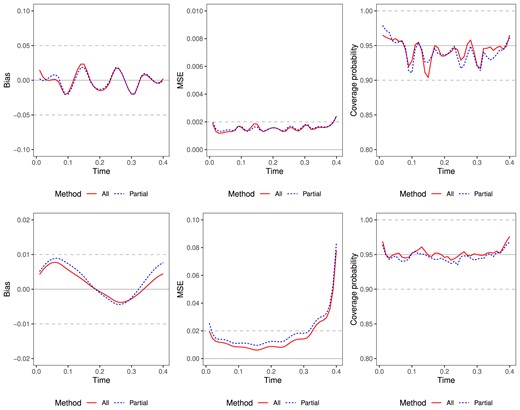
Simulation results of estimated trajectories for normal data (top) and zero-inflated gamma data (bottom). n = 4000, x = (0,0), s = 0.4. Left: plots of point-wise biases; middle: plots of point-wise mean squared errors; right: plots of pointwise empirical coverage probabilities. We compare lines for methods using all data (red solid) or using partial data (blue dashed).
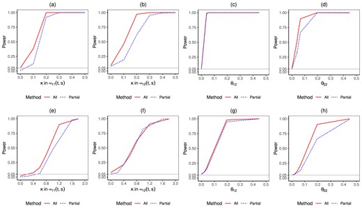
Simulation results of estimated power curves for normal data (top) and zero-inflated gamma data (bottom). n = 4000, x = (0,0), s = 0.4. We compare lines for methods using all data (red solid) or using partial data (blue dashed).
Bias, MSE and CP of linear coefficients in the simulation studies.
| Example 1: normal data | |||||||
|---|---|---|---|---|---|---|---|
| All data | Partial data | ||||||
| n | Bias | MSE (× 10−2) | CP | Bias | MSE (× 10−2) | CP | |
| 2000 | θ11 | −0.001 | 0.018 | 0.935 | 0.001 | 0.019 | 0.951 |
| θ12 | −0.001 | 0.018 | 0.935 | 0.001 | 0.019 | 0.951 | |
| θ21 | −0.001 | 0.079 | 0.937 | −0.003 | 0.158 | 0.937 | |
| θ22 | 0.001 | 0.077 | 0.941 | 0.001 | 0.150 | 0.938 | |
| 4000 | θ11 | −0.001 | 0.008 | 0.949 | −0.001 | 0.009 | 0.947 |
| θ12 | 0.001 | 0.008 | 0.946 | 0.001 | 0.009 | 0.948 | |
| θ21 | −0.001 | 0.040 | 0.935 | −0.001 | 0.074 | 0.947 | |
| θ22 | 0.001 | 0.040 | 0.932 | 0.001 | 0.073 | 0.944 | |
| Example 2: zero-inflated gamma data | |||||||
| All data | Partial data | ||||||
| n | Bias | MSE (× 10−2) | CP | Bias | MSE (× 10−2) | CP | |
| 2000 | θ11 | −0.011 | 0.526 | 0.942 | −0.016 | 0.830 | 0.907 |
| θ12 | 0.004 | 0.459 | 0.935 | 0.005 | 0.702 | 0.887 | |
| θ21 | −0.013 | 0.922 | 0.921 | −0.029 | 2.032 | 0.901 | |
| θ22 | 0.001 | 0.808 | 0.916 | 0.003 | 1.567 | 0.888 | |
| 4000 | θ11 | −0.005 | 0.257 | 0.930 | −0.008 | 0.376 | 0.913 |
| θ12 | 0.002 | 0.241 | 0.933 | 0.003 | 0.335 | 0.926 | |
| θ21 | −0.005 | 0.403 | 0.935 | −0.012 | 0.875 | 0.925 | |
| θ22 | −0.001 | 0.382 | 0.938 | −0.001 | 0.781 | 0.925 | |
Data generated from normal distribution and zero-inflated gamma distribution in examples 1 and 2.
In Table 2, when the outcomes follow a multivariate normal distribution, we see that the coverage probabilities for index parameter estimates are close to the nominal 95% confidence level. The bias is small, and the MSE decreases as the sample size increases. Compared to the method using only uncensored or LTS (partial) data, the method using all data reduces the MSE. For example, when n = 2000, the MSE of θ21 reduces by 50% when cost data from censored subjects is used. This indicates that properly accounting for censoring is particularly beneficial for improved efficiency when the number of observations is relatively small.
When the outcomes follow a zero-inflated gamma distribution, the bias for index parameter estimates is small, and the MSE decreases as the sample size increases. This decrease indicates that the proposed estimation under the identity link function is robust against skewness and zero-inflation. This is because it does not model the full distribution of the cost data. The coverage probabilities for the method using partial data are slightly less than 95%, but close to 90% when the sample size is 2000. The coverage probability is closer to 95% when censored cost data is used, and the estimates of the confidence interval become more accurate as sample size increases.
Figure 4 visualizes the simulation results of the estimated baseline trajectories for examples 1 and 2 when n = 2000 at terminal event times s = 0.4 and baseline covariates x = (0,0). We see that the coverage probabilities are close to the nominal 95% confidence level. The pointwise bias and MSE are both small, suggesting that the proposed estimator fits the baseline trajectory well. As expected, the MSE curve for the method using all data is lower as expected. For a few boundary points, MSE is large due to the small bias caused by the limited sample size in those regions.
Lastly, we evaluate the proposed Wald test statistic using the above-mentioned examples. The statistic has two main goals as described in Section 3.6: one is to test whether the shape of the trajectory curves is constant, and the other is to test whether the covariate index parameters equal zero. Figure 5 shows the power function curves under the given significance levels. When the outcome is normal, Figure 5a and b shows that the power curves increase rapidly with the non-constant strength κ for μ11(t, s) and μ12(t, s), which are the varying coefficient functions in the proposed 2-part model. The method using all data has better statistical power. When the effect is close to 0, the test sizes are all approximately at the significance level. Figure 5c and d show that the power curve for index coefficients θ12 and θ22, which represents the second index parameter in each part of the model. As the sample size in the partial data method for estimating the θ12 is large, its power is similar to the power of the all data method. The second row of Figure 5 indicates similar findings for zero-inflated gamma data. Additional simulation in Web Appendix for multivariate gamma and zero-inflated normal data shows unbiased estimation of both index coefficients and trajectory functions. Additional simulations that evaluate the proposed method under various settings with different censoring rates are presented in Web Appendix Section 3.
6 DISCUSSION
In this paper, we propose a longitudinal varying coefficient single-index model to detect and test for the complicated nonlinear relationships between the longitudinal medical cost trajectory and baseline covariates in the presence of right-censoring. This model helps health services researchers and policy-makers understand how the baseline patient and initial treatment characteristics affect the shape of subsequent cost trajectories given their survival time. Since the healthcare costs are related to both the time since the initial diagnosis and the survival time, which is subject to right-censoring, the model has to account for both. To our knowledge, there have been no published statistical methods for this problem. Our model formulation balances the consideration of research objective, flexibility, parsimony, and interpretation. The estimation is robust against a distribution assumption of the cost data or incorrect modeling of the within-subject correlation. From a methodological perspective, this is an extension of GEE to incorporate censored covariates.
One advantage of the proposed method is that a consistent initial estimator can be obtained by analyzing the uncensored subjects and LTS. This is helpful from a computational perspective because the data analysts can quickly fit the model using standard software. The estimation efficiency and statistical power can be significantly improved by using data from censored subjects, who can be a large proportion in any real-world dataset. This final analysis can be completed by using the proposed method in this paper and our specialized program. We will make the R code that implements the proposed method for the simulation study and data analysis available to the public. Furthermore, the proposed method has broad and rich interpretations through not only numeric tables, 2D / 3D figures, but also an extended use of nomogram, which serves as a translational tool to accommodate the proposed models in a visually interpretable way.
There are some different results of covariate effects for patients who died within vs. over 40 quarters (eg, using surgery as an initial treatment) in the data example, possibly because multiple factors may dilute the cost across patients’ lifespans. Thus, evaluating the relationship between cost trajectory and time-dependent covariates such as cancer progression and the definitive treatments will be important for subsequent research. The statistical literature in the field of cost-effectiveness has been deficient in addressing the potential changes in cost-effectiveness over time. To address this gap, we put forth a semiparametric estimator and variance that can serve as a foundation for further research into the time-varying cost trajectory in relation to baseline covariates. Future work in this area might develop a methodology for the measure of cost-effectiveness.
Funding
This research is supported by NIH grants R01CA225646 and P30CA016672, and CPRIT grant RP210130.
Conflict of interest
None declared.
Data availability
The data that support the findings of this paper are available from SEER-Medicare. Restrictions apply to the availability of these data, which were used under license for this paper. Data are available at https://healthcaredelivery.cancer.gov/seermedicare/ with the permission of SEER-Medicare.
