


Abstract
The transmission rate is a central parameter in mathematical models of infectious disease. Its pivotal role in outbreak dynamics makes estimating the current transmission rate and uncovering its dependence on relevant covariates a core challenge in epidemiological research as well as public health policy evaluation. Here, we develop a method for flexibly inferring a time-varying transmission rate parameter, modeled as a function of covariates and a smooth Gaussian process (GP). The transmission rate model is further embedded in a hierarchy to allow information borrowing across parallel streams of regional incidence data. Crucially, the method makes use of optional vaccination data as a first step toward modeling of endemic infectious diseases. Computational techniques borrowed from the Bayesian spatial analysis literature enable fast and reliable posterior computation. Simulation studies reveal that the method recovers true covariate effects at nominal coverage levels. We analyze data from the COVID-19 pandemic and validate forecast intervals on held-out data. User-friendly software is provided to enable practitioners to easily deploy the method in public health research.
1 Introduction
Infectious diseases present a threat to public health, and their potential impact is increasing with accelerating global travel and urbanization. Thus, it is important that we use each new disease outbreak as an opportunity to improve our preparedness for future pathogen outbreaks. One way to improve our capacity to fight future infectious disease outbreaks is to develop statistical methods which enable the use of surveillance data to (1) quantitatively estimate the relative impact of different public health interventions and (2) compute short-term, localized forecasts for the infectious disease burden. Methods satisfying these criteria would facilitate timely, targeted interventions by public health officials and would empower high-risk individuals to manage their exposure risk. We will refer to statistical methodologies developed with these aims as examples of epidemic regression analysis.
In this paper, we aim to develop a methodology tailored to the features and deficiencies exhibited by many of the large-scale epidemic surveillance data sources during the COVID-19 pandemic. We anticipate major sources of bias and uncertainty will be difficult to eliminate from rapid-response data collection efforts for novel and resurgent epidemics in the near future, especially in developing regions (Vasudevan et al., 2021), suggesting that ours and similarly motivated methodologies will remain relevant in making sense of such data sources. We illustrate use of this method through application to an assemblage of several contemporary data sources: the county-day resolution incidence data compiled by The New York Times (2021), the state-day resolution vaccination data compiled by Our World in Data (2022), and clinical data from several authors, as we elaborate in the Supporting information, Section C.1.
The conceptual starting point for many infectious disease models is the idea that the population can be partitioned into compartments (e.g., susceptible or infectious) and that new infections are proportional to both the susceptible and infectious populations (Hamer, 1906; Kermack & McKendrick, 1927). This line of reasoning was developed throughout the 20th century in deterministic and stochastic compartmental model formulations, as summarized by Hethcote (2000) and Andersson and Britton (2000), respectively. Efforts to improve forecasting of annual influenza disease burden have been a major driver of methodological innovation (e.g., Osthus & Moran, 2021 and references therein) though some of the associated methodology relies on recurring seasonal patterns. Other recent contributions to the literature can be organized as responding to two thematic challenges.
First, there is the challenge of devising a parsimonious model which is also plausible, particularly since we observe the sequential incidence data with subtle error processes (Tang et al., 2020). Adopting a state space structure allows us to flexibly and interpretably model a sampling density separately from the evolution of the population. Furthermore, we can prevent measurement error from contaminating infection dynamics, unlike observation-driven models (Cox et al., 1981). Well-known examples of state-space modeling include Shaman and Karspeck (2012) and Dukic et al. (2012). The compelling DBSSM model of Osthus et al. (2017) has been extended by Wang et al. (2020) and Zhou et al. (2020). However, many of these models have adopted unrealistic sampling models, assuming that surveillance data provide unbiased observations of the infectious compartment. For examples of more realistic sampling models, see Johndrow et al. (2020) or Quick et al. (2021).
Second, while the mathematical models of disease recapitulate certain realistic properties of epidemic transmission, they yield poor stand-ins for real-world transmission. For example, they typically anticipate a single wave of infection, whereas often multiple waves of infection are observed in practice (Patterson & Pyle, 1991; Orsted et al., 2013; Karako et al., 2021). The most intuitive solution to this problem is to allow transmission parameters to vary over time, often either the transmission rate or the basic reproduction number in particular.
Examples of flexible transmission rate modeling, along with attempts to associate changes with covariates, include Wallinga and Teunis (2004), Cori et al. (2013), and Thompson et al. (2019). These models suffer the drawback of placing no temporal correlation structure on the transmission rate, instead relying on windowed estimates to achieve smoothing behavior, and furthermore they are observation-driven. Hespanha et al. (2021) devised a forecast methodology for COVID-19 by modeling parameters with random walks.
In contrast, the “eSIR” model (Wang et al., 2020) is a state-space model based on the DBSSM which allows a time-varying transmission rate which can be associated with covariates. The eSIR authors published a software package of the same name, and their methodology has been deployed and extended in various contexts (Zhou et al., 2020; Ray et al., 2020); however, the time-varying transmission rate is assumed to have a known functional form as a simple combination of basis functions. Similar limitations are present in Johndrow et al. (2020) and others who model transmission rate as a piecewise function. Keller et al. (2022) developed a sophisticated methodology for estimating covariate effects with a smooth temporal deviation and a multiplicative process for state-evolution error.
Some large scientific collaborations succeeded in applying impressively complex models to effect estimation and forecasting tasks (e.g., Monod et al. 2021; IHME COVID-19 Forecasting Team, 2021), but these relied on ad hoc procedures for fitting and quantifying uncertainty. Moreover, there is limited software available to reproduce such analyses and the methods would be exceedingly difficult to port to other problems. The MERMAID methodology proposed in Quick et al. (2021) learns a smooth transmission rate as a function of covariates and spline terms but amplifies the likelihood contribution of seroprevalence data in order to achieve identifiability.
Recent and continued methodological advances appear to demand careful design of posterior computation algorithms. Johndrow et al. (2020) implemented an adaptive Metropolis algorithm (Haario et al., 2001) to facilitate rapid mixing of their iterative MCMC sampler. Zhou and Ji (2020) fitted a latent Gaussian process (GP) model using a Parallel Tempering MCMC algorithm (Woodard et al., 2009; Miasojedow et al., 2013), but did not incorporate a hierarchy to borrow information across parallel streams of incidence data, and reported challenges with covariate effect estimation. Keller et al. (2022) invoked HMC sampling algorithms implemented via Stan (Carpenter et al., 2017).
In this paper, we describe a novel model and computational algorithm for epidemic regression analysis. Our hierarchical, semi-parametric regression model is to our knowledge unique in the literature. We use latent GP priors to achieve smooth temporal random effects rather than the splines often used for that purpose. Moreover, several articles have discussed the potential value of hierarchical priors on covariate effects to enable borrowing of information across regions, but do not provide implementation. We achieve robust posterior computation for our model by taking advantage of techniques developed in the literature for Spatial Generalized Linear Mixed Models (SGLMMs) (Diggle et al., 1998). Our methodology is accessible to practitioners through an open-source, user-friendly R package smesir (2022), available on GitHub.
The remainder of the paper is organized as follows. In Section 2, we describe our data, notation, and model. We summarize the results of extensive simulation studies in Section 3 and highlight results from application to the COVID-19 epidemic in Section 4. We conclude with discussion of future work in Section 5. Additional results, sensitivity analyses, extended description of our methodology, and detailed description of our posterior computation algorithm are presented in the Supporting information.
2 Methods
2.1 Data and Notation
In this paper, we will be working with panel format incidence data, for which individual observations might be counts of new cases, new hospitalizations, or deaths that occur in a specific population during a given time interval. To avoid unnecessary loss of generality, we will refer to any such data as counts of incidence events or, simply, events.
We suppose that the data are observed for K non-overlapping regional populations over a sequence of T contiguous, equal-length time intervals. We then suppose the incidence data are arranged into a  matrix
  of non-negative event counts. Additionally, we may optionally have P covariates of interest, arranged into a
  tensor
  of covariate values such that each of the
  covariate series is centered and scaled. If a vaccine is available, our model will take vaccinations into account via a
  matrix
  of non-negative counts of newly vaccinated individuals. We adopt the indexing convention that a contiguous slice of values
  may be abbreviated as
  . Bold notation will be used to indicate that indices have been suppressed for at least one dimension of a multidimensional variable, for example
  or
or  . Finally, we will use bold
  to denote a vector of ones and
  as the indicator function.
We use an integer index over sequential observations, aligning indices,  , to the specific times,
  , at which event counts were reported in our data. Epidemic event counts or covariate values reported at
  should reflect circumstances from the interval
  , and where no confusion is possible, we refer to these intervals by the index of their associated reporting time. Hence,
  and
and  are referred to as observation time i and interval i, respectively. For sequential indices less than 1 or greater than T, we assume that the constant time-interval width is maintained. We define the regional outbreak times as the collection
  such that
  if the first case in region k was reported during interval i. Since the first reported cases should precede or coincide with reports of any other type of event, for each region k we assume
  for all
  .
.
Finally, we will adopt the convention of presenting Gaussian distributions ( ) in the mean-variance parameterization, half-Gaussian distributions (
 ) in terms of the variance parameter of the corresponding unfolded Gaussian, gamma and inverse-gamma distributions (e.g.,
  ) in the shape-rate parameterization, exponential distributions (
 ) in the rate parameterization, Poisson distributions (
 ) in terms of their mean, and negative binomial distributions (
 ) in terms of a mean and a dispersion parameter.
2.2 Review of Compartmental Epidemic Models and the Empirical Transmission Rate
A popular class of mathematical models for infectious disease is compartmental models. Abstractly, such models break a population into distinct compartments and specify rules by which portions of the population transition between compartments. A concrete example is the highly popular SIR model, named for its proposed division of the population into Susceptible, Infectious, and Recovered (immune) compartments (Kermack & McKendrick, 1927).
The transition rules of the original SIR model can be encoded as a system of discrete-time difference equations  ;
;  ; and
; and  ; where β is the transmission rate, γ is the recovery rate, and t is an index over time. The variables
  , and
, and  represent the sizes of the compartments at index time t, measured as fractions of the population. Note the key term
  determines the portion of the population newly infected at time t in this model.
As discussed in Section 1, many fixed parameter compartmental models fail to anticipate the multiple waves of infection frequently observed in disease outbreaks. A simple way to induce the SIR model to admit these trajectories is by supposing the transmission intensity between susceptible and infectious populations can vary over time due to viral or host evolution, environmental, or behavioral factors. Following this line of reasoning, we replace the static parameter β with a dynamic empirical transmission rate parameter,  . We usually refer to this variable simply as the transmission rate, but emphasize here that we are describing the realized rate at which a disease is being transmitted through the population, driven both by biology and behavior, and not the notion of an inherent “biological” transmission rate.
2.3 State-space Modeling and the Production Process
We call the proportional compartment populations (i.e.,  from the preceding discussion) the state of the population at time t. Unfortunately, measurements of the population state, such as seroprevalence studies to estimate
  , can be difficult to obtain and biologically unreliable (Muecksch et al., 2021). Instead we must often rely on incidence data to provide indirect information about the population state based on their relationship with state transitions, like the portion of the population newly infected during interval t.
In what follows, we will to refer to any probabilistic model for incidence data given recent infections as a production process. We let  represent the number of individuals newly infected during period t. Note that while new infections appear to be modeled as a deterministic function of the population state, randomness will be injected into the infection series via stochastic evolution of the transmission rate. A production process can be written in general terms as
  , where
  is the incidence count data for a particular population at time t,
  is a family of probability distributions indexed by θ, and θ is a collection of relevant production parameters such as the infection fatality rate, testing rate, or a distribution of lag times from event detection to reporting. The types of quantities that must be included in θ will depend on whether the incidence data
  are cases, deaths, or some other type of incidence event.
To define the process  , we follow the reasoning in Johndrow et al. (2020). Suppose at first that
  is Poisson, and the mean is a weighted linear function of recent infection counts, so
  where
where  is a weighted sum over recent new infections. Specifically,
  such that
  is the probability that an infected individual will contribute to the reported incidence event count m intervals after the interval during which they were infected. We assume that there is a maximum production lag, M, so that
  for
for  , and that
  .
.
The production parameters θ and corresponding weights  will not be known exactly, nor do we hope to estimate them within our methodology. Therefore, ultimately we will not employ a model for
  but rather
  , where
  is an estimate of the production weights which we obtain from clinical or administrative data,
  , prior to our analysis. We can obtain the latter distribution by marginalizing
  over conditional uncertainty
  , leading to an overdispersed count distribution for
  . Specifically, it is convenient to model our uncertainty by supposing that
  , where
  is gamma distributed with mean 1 and variance
  . Then, we find the simple expression for the observation distribution
  . Example specifications of
  based on clinical data are given in the Supporting information and applied in Section 4.
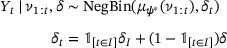
In our model, the dispersion parameter is typically assumed to be a fixed value,  for all t, and δ will be learned from the data. However, epidemic incidence data might feature “corrupted” intervals I for which we have very low confidence in our estimate
  or otherwise suspect poor data quality. In such instances, to avoid over-fitting it may be reasonable to set a hyperparameter
  and assert
  for any
  . We frequently let
  , which loosely corresponds to assigning a 95% probability to the fact that
  is within an order of magnitude of the most appropriate values.
The combination of the flexibly specified approximate acquisition probabilities  , the corrupt-data flag I, and the corrupt-data over-dispersion parameter
  were meant to accommodate some of the irregularities of surveillance data observed during the COVID-19 pandemic. Notably, the realized lag times from an infection to a case report, hospitalization, or death, appeared to depend on uncertain biological characteristics as well as technical hurdles. In particular, for case detection, the most appropriate acquisition probabilities
  likely evolved substantially over geographic regions as well as short- and long-term time horizons due to test availability, symptomatic/asymptomatic test policy, and pervasive, observable intra-week reporting probabilities. In Section 4, we will show that a calibrated application of our strategy achieves our modeling objectives, imputing appropriate (large) uncertainty while still enabling us to extract some meaningful inferences from large data, while simulation studies described in Section 3 suggest the validity of our inferences is not substantially degraded by poor choices of
  .
.
2.4 Single-region Statistical Model
We have already outlined the rationale for our model in Sections 2.2 and 2.3. In this section, we formally describe our model for a single region, temporarily eliminating the need for the spatial indices  described in Section 2.1. We will extend the model to accommodate panel data from multiple regions in the subsequent section. Implementations of both the single-region model described in this section and the multi-region model described in the next section are provided in our open source R package smesir (2022). A detailed development of our algorithm for posterior computation, building on techniques developed in the spatial statistics literature, is provided in Section A of the Supporting information.
For our observation model, we assume that the sequential event counts  are jointly independent given the trajectory of new infections
  and that
  given
given  is independent of
  for all t. Then,
where, here and afterward, for conciseness, we will no longer explicitly condition on quantities which will not be inferred from the data—in the above,  , I, and
  —because those values are assumed to be fixed in advance as part of the model, just as the negative binomial family is fixed in advance.
Our state-evolution model extends the SIR model by assuming a time-varying transmission rate, and also introducing direct transfers from the susceptible to the removed compartment via vaccination. We denote the proportion of the population which is unvaccinated as of time t with  , while the proportion of the population which is newly vaccinated during interval t is designated as
  . We assume that vaccines are administered independently of whether a person has previously been infected, but that previously vaccinated individuals are not vaccinated again. We also assume that vaccines confer immunity which is indistinguishable from prior infection. This leads us to the following set of state evolution equations:

For readability we have omitted min/max operators which are necessary to enforce, for example, that the implied new infections do not exceed the size of the susceptible compartment. We set the initial condition of the state to  , where o is defined as in Section 2.1 and ι is the unknown initial infectious population which accounts for the detected cases at time o. We assume
  for
for  . Note that this model treats the system as though it were closed. Implicitly we rely on a moderately large population size and sufficiently short observation time so that births, non-disease related deaths, immigration, and emigration do not contribute substantially to the evolution of the system. For modeling purposes, disease-related deaths can be conflated with acquired immunity so long as neither group is expected to transmit disease.
We note that this state-evolution model is inappropriate for endemic infectious diseases, for which immunity decay may become a significant dynamic. However, we contend that it is a reasonable model for many early-stage epidemics, including the COVID-19 outbreak through the end of 2021, during which time full vaccination and prior infection seemingly conferred robust, medium-term immunity to the extant viral strains. We discuss the need for model extensions and rigorous comparative model evaluation in Section 5.
We adopt a semiparametric log-linear mixed-effects model for  to capture covariate-explained and unexplained temporal heterogeneity,
  , where α is an intercept term,
  is a vector of coefficients, and
  is a vector of temporal random effects. Specifically, we suppose that the random effect
  is the value of an unknown smooth function
  evaluated at time t, and model the function as a draw from a GP
  such that
  is the squared exponential kernel with lengthscale parameter ℓ.
As discussed in Melikechi et al. (2022), models which feature both the transmission rate and recovery rate as free parameters are not always practically identifiable. Therefore, we assume that the population size N, recovery rate γ, and estimated production weights  are available to the user or can be reasonably estimated via some external procedure. We demonstrate elicitation of these parameters from clinical data in an analysis of U.S. COVID-19 data in Section 4. For computational convenience, we also require the lengthscale parameter of the random effect (ℓ) to be specified in advance based on intuition for how rapidly temporal dependence in the random effect
  should decay.
Taking a Bayesian approach to inference, we construct a joint prior as a product of independent marginals. By default, we adopt somewhat informative priors consistent with properties of observed epidemics:  ,
,  ,
,  ,
,  , and
, and  . Our software allows specification of more diffuse priors, if desired.
2.5 Multi-region Statistical Model
Our model accommodating panel data from multiple regions are a direct hierarchical extension of the single-region model proposed in Section 2.4. Specifically, for  , we have local population size
  , initial infectious population
  , outbreak times
  , vaccination proportion time series
  , and transmission rate models
  that collectively determine the region's state evolution:
  for
for  , then
  when
when  , and finally according to the system of equations in display (2) for
  . The differences across regions in the parameters of the log-linear model for
  can be interpreted as capturing differences due to population density, degree of compliance with public health mandates, or other unmeasured behaviors. Similarly, we assume that local hyperparameters
  are available and model observed regional event counts
  as conditionally independent across regions given local infection counts
  and dispersion parameters
  .
.
Our hierarchical prior structure reflects our belief that knowing the region-specific intercept and effects for the transmission rate in one region will provide information about the analogous parameters for the other regions, in the sense that they will be scattered around central, “global” parameter values. Hence, for  , we have
  ,
,  and
and  . We place weakly informative priors on the hyperparameters of this hierarchy, specifically
  ,
,  , and
, and  . Priors on the initial infectious populations and dispersion parameters are independent across regions
  and
and  .
.
3 Simulation Study
To evaluate performance of our model and computational approach in recovering covariate effects, we conducted an in-depth case study of a simulated dataset as well as a broad simulation meta-analysis. In the case study, we generate and analyze a single, simulated, multi-region epidemic dataset. In the meta-analysis, we randomly generate 1,000 sets of model parameters and estimate the empirical coverage rate and concentration of our 95% posterior credible intervals. The results of our investigation of coverage rates when data are generated under the model are presented in Table 1, while details about our simulation studies and extended results, including estimates of empirical coverage rates when hyperparameters are misspecified, are available in the Supporting information, Section B. Overall, these studies demonstrate satisfying coverage properties of Bayesian credible intervals when data are simulated from the model, and show that performance is robust to errors in specification of the recovery rate γ and the production weights  .
.
Coverage rates of quantile-based 95% credible intervals for each parameter.
 | 2 | 3 | 4 | 5 | 0 | |
|---|---|---|---|---|---|---|
 | 98 | 98 | 97 | 97 | 97 | 97 |
 | 97 | 99 | 97 | 97 | 98 | 97 |
 | 92 | 94 | 91 | 92 | 93 | 93 |
 | 94 | 93 | 93 | 94 | 93 | 93 |
 | 97 | 95 | 97 | 96 | 94 | |
 | 95 | 95 | 95 | 95 | 93 | |
 | 97 | |||||
 | 94 |
| 2 | 3 | 4 | 5 | 0 | |
|---|---|---|---|---|---|---|
| 98 | 98 | 97 | 97 | 97 | 97 |
| 97 | 99 | 97 | 97 | 98 | 97 |
| 92 | 94 | 91 | 92 | 93 | 93 |
| 94 | 93 | 93 | 94 | 93 | 93 |
| 97 | 95 | 97 | 96 | 94 | |
| 95 | 95 | 95 | 95 | 93 | |
| 97 | |||||
| 94 |
Note: Coverage rates are computed over 1,000 simulated datasets, each with  ,
,  ,
,  , and a distinct (random) set of parameters. Column headings specify the pertinent region (0 for global parameters). Row labels specify the parameter.
Coverage rates of quantile-based 95% credible intervals for each parameter.
| 2 | 3 | 4 | 5 | 0 | |
|---|---|---|---|---|---|---|
| 98 | 98 | 97 | 97 | 97 | 97 |
| 97 | 99 | 97 | 97 | 98 | 97 |
| 92 | 94 | 91 | 92 | 93 | 93 |
| 94 | 93 | 93 | 94 | 93 | 93 |
| 97 | 95 | 97 | 96 | 94 | |
| 95 | 95 | 95 | 95 | 93 | |
| 97 | |||||
| 94 |
| 2 | 3 | 4 | 5 | 0 | |
|---|---|---|---|---|---|---|
| 98 | 98 | 97 | 97 | 97 | 97 |
| 97 | 99 | 97 | 97 | 98 | 97 |
| 92 | 94 | 91 | 92 | 93 | 93 |
| 94 | 93 | 93 | 94 | 93 | 93 |
| 97 | 95 | 97 | 96 | 94 | |
| 95 | 95 | 95 | 95 | 93 | |
| 97 | |||||
| 94 |
Note: Coverage rates are computed over 1,000 simulated datasets, each with , , , and a distinct (random) set of parameters. Column headings specify the pertinent region (0 for global parameters). Row labels specify the parameter.
4 Application
To illustrate the use of the smesir package in explaining and forecasting the transmission rate, we analyze surveillance data from the COVID-19 epidemic in the 50 U.S. States. In particular, we use data from a repository we maintain (U.S.A. COVID-19 Data, 2022), which has been cleaned and processed to smooth out recording errors and artifacts due to within-week reporting cycles and other idiosyncrasies. Complete details, along with references to raw data sources and reproducible code for recreating the data files are also made available in that repository. Since the repository is updated periodically as new data are published, to ensure that the following analysis is reproducible we have included an exact copy of the data analyzed in our software package, smesir.
We select reasonable values for epidemiological parameters by considering side information from demographic reports and clinical studies. The full elicitation of our epidemic parameters and the production weights  is presented in the Supporting information, Section C.2, and a sensitivity analysis wherein we examine the impact of these choices on our conclusions by repeating our study under various plausible alternative specifications is presented in Supporting information, Section C.4.
Motivated by the widely publicized challenges in data collection throughout the pandemic (Dean & Yang, 2021), coupled with the fact that uncertain demographic composition of the recently infected population could have a large effect on the production process (e.g., the average age of the newly infected population would have a massive impact on the realized infection fatality rate) we set  and let
  , the complete set of observation times. We fix a lengthscale of 8 weeks in the squared-exponential covariance function of our temporal random effect, on the basis that large, unexplained swings in behavior seem unlikely to occur within time frames less than a month or so. Otherwise, we use the default prior specification as described in Section 2.5.
We generated samples from the posterior distribution of our parameters using the smesir package with default settings. The convergence diagnostics  and effective sample size (Gelman et al., 2013), which are computed automatically within the smesir package, provided no evidence that the Markov chains failed to converge.
4.1 Effect Estimation
To demonstrate the estimation of covariate effects in practice we consider the impact that the emergence of the Delta variant had on the state-level transmission rates.
One example of how we can use our model to probe the relationship between the transmission rate and a covariate is by first modeling the log transmission rate with only the intercepts  and GP temporal random effects
  . We use the posterior means as point estimates
  and plot them against the corresponding covariate values to visualize the marginal relationship. This approach may be of exploratory value when the relationship between the transmission rate and the covariate of interest is possibly not log-linear. We construct such a plot for our analysis of the Delta variant effect in Figure 1, excluding the many points where the prevalence covariate was exactly 0 or 1 for clarity.
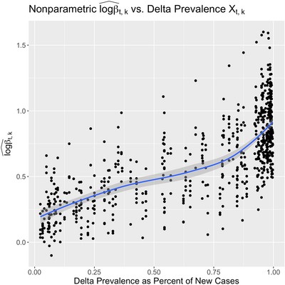
Scatter plot of non-parametric estimates of the instantaneous local transmission rate  vs. the local prevalence of the Delta variant as a percent of new cases during the same time period. A loess line is superimposed to highlight the apparent nonlinear trend. This figure appears in color in the electronic version of this paper.
In Figure 1, we see that the log transmission rate seems to increase super-linearly with delta prevalence, and so we fit our full semiparametric model with squared prevalence as a covariate. In Figure 2, we visualize how our posterior distribution of the Delta variant's “global” effect ϕ0 on transmission rate concentrates as the amount of data observed increases. To do this, we fit our model twice—including the first 6 and then 19 weeks after the Delta variant first appeared in the United States. We summarize the final posterior distribution for all 50 of the local coefficients  in Figure F of the Supporting information.

This collection of superimposed histograms illustrates the progressive posterior concentration for the effect of the Delta variant prevalence on transmission rate. Specifically, this coefficient is associated with the squared proportion of Delta variant infections among recent new COVID-19 cases. The three histograms show the N(0, 10) prior distribution (with upper and lower tails cropped out for clarity), the posterior distribution after week 77 (6 weeks after the Delta variant first appeared in the United States), and the posterior distribution after week 90. This figure appears in color in the electronic version of this paper.
4.2 Forecasting
To demonstrate the forecasting performance of our method in a context where relevant covariates and vaccination data are both available, we again focus on the period just before and immediately after the appearance of the Delta variant in the United States. Since alternative methods do not admit vaccination data, we cannot compare our methodology to related approaches for this particular example. Instead, in Section D of the Supporting information we include an additional forecast analysis which highlights the strength of our forecast uncertainty quantification relative to a state-of-the-art alternative.
In the late spring and early summer of 2021, as vaccination rates increased and, in many places, social distancing measures were still in effect, new cases and deaths from COVID-19 were rapidly declining in the United States. Indeed, from these incidence data alone it appeared that, locally, the COVID-19 epidemic was coming to a close. However, with the easing of public health interventions and the emergence of the new, more transmissible Delta variant, cases, and eventually deaths, surged again as the summer ended. The sudden turn of events allows us to ask whether our method can detect a change in the underlying dynamics of disease transmission before a trend reversal is visually evident in the incidence data. To see this, we compare the forecast distributions of the model fit separately to the first 74 and 77 weeks of data—the former model is fit without an effect for the Delta variant prevalence as the covariate had been essentially zero up to that time.
To summarize our results, we sum the forecasts from all 50 states to obtain a forecast distribution for the entire U.S. population. The 90-week time series of weekly death totals for the combined 50 States, plus the forecast intervals for the model fit to the first 74 and 77 weeks of data, are plotted in Figure 3. While the 95% forecast intervals after 74 and 77 weeks both accommodate the surge in deaths associated with the Delta variant, we can make a more detailed comparison by identifying the quantile of the forecast distribution which most closely matches the observed data. Indeed, the actual course of death counts observed in late summer was regarded as being much more plausible after 77 weeks than after 74 weeks (see the comparison of the pointwise event forecast quantiles in Figure 3), despite the fact that incidence of deaths had declined in that 3-week period. Evidently, the stalling decline in deaths served as evidence that the transmission rate was actually increasing.
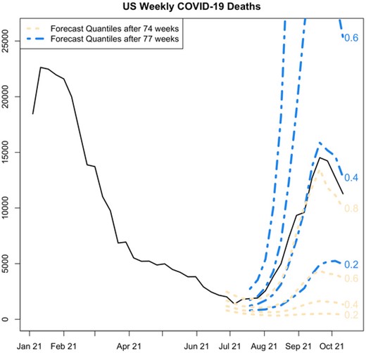
Comparison of forecast distributions after the first 74 and 77 weeks of the U.S. COVID-19 epidemic. Parallel pointwise forecast quantiles are labeled with their associated probability level. Note that, while both forecast distributions admit the possibility of a surge in deaths, the eventually observed surge in deaths is seen as much less surprising at 77 weeks, despite the fact that weekly deaths fell between weeks 74 and 77. This suggests that our model is not only sensitive to the current counts of deaths but also to the larger context of evolving rates of change. This figure appears in color in the electronic version of this paper.
5 Discussion
It is possible that sequential algorithms for posterior computation may be suitable for fitting our model. Such tools would be appealing as the length of the incidence data history increases, since they obviate the need to completely retrain the model as new observations are obtained. Sequential algorithms were developed in both Shaman and Karspeck (2012) and Dukic et al. (2012). An additional strength of some sequential Monte Carlo algorithms is their ability to be parallelized (Durham & Geweke, 2014).
In this paper, we have described an innovative methodology for analyzing and forecasting multi-region epidemic incidence data, and contextualized that contribution within the rapidly evolving literature. Our software tool should facilitate retrospective analysis of the international COVID-19 pandemic as well as forecasting in the early stages of future infectious disease outbreaks. There are several areas for future work. First, the spatial literature we relied on to design our posterior computation algorithm includes other techniques which we have not yet explored in this context, such as random-projection algorithms for matrix inversion (Banerjee et al., 2013; Guan & Haran, 2018) and additional reparameterizations (Christensen et al., 2006) which might enable robust sampling of more parameters including the GP lengthscale and a larger number of linear coefficients.
Another direction for future work is expansion of the state evolution model itself. Minimally, it seems essential that immunity decay be introduced in order to express the full course of COVID-19 transmission dynamics. Another direction would be to introduce flows of transmission between regions, legitimizing the application of our model to higher spatial resolutions. Some work in this direction can be found in von Neumann and Burks (1966), White et al. (2007), and Zhou et al. (2020). Beyond that, we would like to rigorously elucidate how and when additional complexity in the state space model is warranted. In at least one instance, Roda et al. (2020) found a simple SIR model outperformed a four-compartment Susceptible, Infectious, Exposed, Removed (SEIR) model when evaluated using the Akaike information criterion (AIC).
Data Availability Statement
The data used in this paper are available in the R package smesir (2022). These data were derived from several resources available in the public domain. For details, see U.S.A. COVID-19 Data (2022).
Acknowledgments
The authors would like to thank the editor, associate editor, and referee for their insightful comments, which motivated substantial improvements in the quality of the manuscript. The research was funded by NIH grant R01-ES028804 from the National Institutes of Environmental Health Sciences.
References
Supplementary data
Web Appendices, Tables, and Figures referenced in Sections 1, 3, and 4 are available with this paper at the Biometrics website on Wiley Online Library, along with a permanent archive of software, data, and instructions to reproduce all results.
Figure A. Plots of each of the four longitudinal covariates used to generate our simulated data in both the simulation case study and our various meta-analyses.
Figure B. The time-varying transmission rates associated with each of five hypothetical regions in our simulation case study.
Figure C. The time series of event counts for each of five hypothetical regions generated for our simulation case study.
Figure D. A demonstration of posterior concentration for various model parameters.
Figure E. A comparison of results from separately fitting the single-region model to each of the five synthetic event count time series in our dataset versus fitting our hierarchical model to the complete dataset.
Figure F. The central quantile-based 95% credible intervals for the effects of the squared fractional prevalence of the delta variant on the COVID-19 transmission rate.
Figure G. Each row summarizes the marginal posterior distribution, under a unique hyperparameter specification, for the hierarchical mean (ϕ0) of the squared delta variant prevalence effects.
Figure H. The sensitivity of forecasts to alternate hyperparameter specifications.
Figure I. A rolling fit of our model to the daily new case data for Texas, which was previously analyzed in Quick et al. (2021).
Figure J. This figure was generated similarly to Figure I, however, in order to facilitate direct comparison with Figure 3 in the rejoinder Quick et al. (2021), we train our model up to December 7, 2020 and summarize the 14-day forecast posterior predictive distribution with the 0.2, 0.5, and 0.8 quantile lines, which were chosen for consistency with the ±1 standard deviation forecast which we believe the reference figure is displaying.
Table A Fixed parameters assumed in our simulation studies.
Table B Posterior concentration: the standard deviation of the marginal prior distribution for each global parameter is listed in the left column, and the corresponding standard deviation of the posterior distribution is listed in the right column.
Table C Coverage rates of posterior quantile-based 95% credible intervals for each parameter when the incident event rate ψ is misspecified ( = 0.9ψ).
Table D Coverage rates of posterior quantile-based 95% credible intervals for each parameter when the duration of the infectious period is misspecified (
= 0.75γ).
Table E Low, middle, and high values considered during our sensitivity analysis for the U.S. COVID-19 deaths analysis results.
