


Abstract
Leveraging information in aggregate data from external sources to improve estimation efficiency and prediction accuracy with smaller scale studies has drawn a great deal of attention in recent years. Yet, conventional methods often either ignore uncertainty in the external information or fail to account for the heterogeneity between internal and external studies. This article proposes an empirical likelihood-based framework to improve the estimation of the semiparametric transformation models by incorporating information about the t-year subgroup survival probability from external sources. The proposed estimation procedure incorporates an additional likelihood component to account for uncertainty in the external information and employs a density ratio model to characterize population heterogeneity. We establish the consistency and asymptotic normality of the proposed estimator and show that it is more efficient than the conventional pseudopartial likelihood estimator without combining information. Simulation studies show that the proposed estimator yields little bias and outperforms the conventional approach even in the presence of information uncertainty and heterogeneity. The proposed methodologies are illustrated with an analysis of a pancreatic cancer study.
1 Introduction
The advent of evidence-based medicine has generated considerable interest in developing methods that can better synthesize information from different sources to infer treatment effects and identify prognostic/predictive factors (Guyatt et al., 1992). The meta-analysis, a quantitative procedure for combining results from multiple relevant clinical studies, is a powerful tool to produce empirical evidence to guide clinical practice (Sutton et al., 2000; Whitehead, 2002). It conventionally refers to methods combining study-level results but has evolved to encompass ones with individual participant data (IPD). The IPD meta-analysis enjoys clear advantages over the conventional aggregate data (AD) meta-analysis because it allows standardization of the endpoint definition, covariates, and analytical methods; it also allows examination of treatment-by-covariate interactions or subgroup analyses. Despite its known advantages, however, IPD meta-analysis is less common in practice because it is more costly and time-consuming; moreover, access to IPD may be a challenge due to privacy concerns and/or administrative problems.
This research is motivated by the growing interest in developing efficient and flexible meta-analysis procedure to integrate IPD and AD (Chatterjee et al., 2016; Chen et al., 2021; Gao & Chan, 2022; Huang et al., 2016; Han & Lawless, 2019; Liu et al., 2014; Zhang et al., 2020; Zheng et al., 2022). When combining information from different sources, challenges arise as AD may be given in different forms and of different degrees of uncertainty. As an example, in a multivariate regression analysis of data from 209 consecutive patients who underwent pancreatectomy at the Johns Hopkins Hospital between 1998 and 2007 to identify prognostic factors for pancreatic cancer survival, the effect of lymph node status, an important prognostic factor, did not reach statistical significance. To improve estimation efficiency, we seek to incorporate the information in the 3-year survival probabilities estimated using 116 patients with different node statuses (Ahmad et al., 2001). It is easy to see that the uncertainty in the external information should not be ignored in the inference procedure because the sample size of the external study is not large. Moreover, a careful examination of the covariate summary statistics revealed that the proportions of margin-positive and node-positive patients in the external study were much lower than that in the internal study, suggesting the presence of heterogeneity in the covariate distribution between the internal and external studies. Our goal is to develop a unified framework that can account for uncertainty in the external study and heterogeneity across different studies simultaneously.
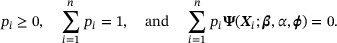
In this paper, we propose an empirical likelihood-based framework for integrating IPD and AD under the semiparametric transformation model. The empirical likelihood method, originally developed for constructing confidence regions (Owen, 1988; Thomas & Grunkemeier, 1975), was later to combine auxiliary information given in the form of moment estimating equations (Qin & Lawless, 1994; Qin, 2000). We aim to exploit t-year survival probabilities, a common form of summary statistics in the context of survival analysis, to improve estimation efficiency and prediction accuracy. Specifically, following Huang et al. (2016), we derive moment constraints by reexpressing the t-year survival probabilities in the form of estimating equations under the semiparametric transformation model. Next, to account for uncertainty in the reported t-year survival probabilities, we exploit the asymptotic normality of summary statistics by treating the reported values as the realization of a normal random vector. This way, the contribution of auxiliary information to the likelihood can be captured by adding a normal density term (Imbens & Lancaster, 1994; Zhang et al., 2020). This augmented empirical likelihood is then maximized subject to the moment constraints derived from the reported t-year survival probabilities to estimate the regression parameters in the semiparametric transformation model. It is worthwhile to point out that, instead of adding a normal density term, a direct extension of the adjusted variance method was proposed by Sheng et al. (2021); however, the latter cannot be easy to handle multiple external studies.
It is known that ignoring important differences between studies can invalidate meta-analysis. In this article, we assume that the covariate effects follow the same semiparametric transformation model but allow distributions of covariates to vary across different studies because they may be conducted in different patient populations with different study designs. To account for the differences in the covariate distribution, which is analogous to the concept of “covariate shift” in transfer learning (Shimodaira, 2000), we employ a density ratio model to characterize population heterogeneity between internal and external studies. To perform empirical likelihood estimation, we reevaluate the moment constraints derived from the summary statistics under the density ratio models of the marginal covariate distributions, in addition to the semiparametric transformation model of covariate effects. Hence, maximizing the augmented empirical likelihood subject to the reevaluated moment constraints can simultaneously account for uncertainty in the reported t-year survival probabilities and population heterogeneity across studies. Of note, the efficiency loss resulting from estimating an additional set of parameters in the density ratio model can be compensated by including additional constraints based on the marginal covariate distribution.
This article is organized as follows. In Section 2, we propose an empirical likelihood method for integrating IPD and the reported t-year survival probabilities under the semiparametric transformation model, where an empirical likelihood is constructed based on a compromise between the pseudopartial and nonparametric likelihoods. In Section 3, we extend the proposed empirical likelihood method to account for the uncertainty in the reported t-year survival probabilities and exploit the semiparametric density ratio model to allow for the population heterogeneity between the internal and external studies simultaneously. The results of simulation studies are provided in Section 4, and the proposed approaches are illustrated by a pancreatic cancer data in Section 5. Finally, some concluding remarks and potential future works are discussed in Section 6.
2 Empirical Likelihood Estimation
2.1 A Brief Review of the Semiparametric Transformation Models
Let T denote the time to a failure event of interest in the internal study. We assume that, conditional on a p-dimensional vector of covariates X, the survival time T follows a semiparametric transformation model

where  is an unspecified monotone function with
  , β is a p-dimensional vector of regression parameter, and ε is a random error with a known cumulative hazard function
  independent of X. Hence, the cumulative hazard function of T given X is
  , with
  and
and  . The semiparametric transformation models encompass the Cox model and the proportional odds model as special cases, where the corresponding random error ε follows the extreme-value distribution and the standard logistic distribution, respectively.
In this article, we impose the usual independent censoring assumption that the time to censoring, denoted by C, is conditionally independent of T given X. Define  and
and  , so that Y gives the observed failure time and Δ is the failure event indicator. The observed data
  are assumed to be independent and identically distributed realizations of
  . Denote by
  the jump of
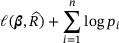
  at time y. Under model (1), the log conditional likelihood is

with  . As pointed out by Zeng and Lin (2006), direct maximization of the conditional likelihood
  is challenging because it involves the nonparametric component
  in a complicated way. Alternatively, an estimator of
  can be constructed by solving the martingale estimating equation

where  is the counting process of the observed failure events and
  is the at-risk process. Specifically, given β, the solution of the martingale estimating equation, denoted by
  , satisfies
Replacing  with
with  in
in  and ignoring a constant term yields the log pseudopartial likelihood (Zucker, 2005)
where  .
.
Define  ,
,  , with
  ,
,  , and
, and  for any vector a. Taking derivative of
  with respect to β yields the pseudopartial likelihood score function
where  . As a result, the maximum pseudopartial likelihood estimator
  can be obtained by solving
  for zero. Denote by β0 and
  the true values of β and
  , respectively. Zucker (2005) showed that
  is asymptotically normally distributed with a zero mean and a variance–covariance matrix
  , where Γ is the negative expectation of the second derivative of the pseudopartial log-likelihood with respect to β and Q is a positive definite matrix resulting from the variation of
  . Moreover, as
  ,
,  converges in distribution to a zero-mean normal distribution with covariance matrix
  . Note that in the special case of the Cox model,
  only involves β and thus Q = 0. As a result, the asymptotic variance of
  reduces to
  . The explicit forms of Γ and Q are given in the Supporting Information.
2.2 An Empirical Likelihood Estimator for Synthesizing External Information
Our goal is to obtain an improved estimation of the semiparametric transformation model by incorporating external information on t-year survival probabilities in different subgroups. We begin by assuming that the uncertainty in the external information is negligible and that subjects in the internal and external studies were random samples from the same population. The two assumptions will be relaxed later in Sections 3.1 and 3.2.
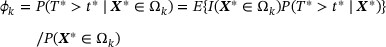
Let  denote the kth subgroup whose survival probability at the time point
  is available from an external study. Let
  denote random variables in the external study. So, the external information can be expressed as
  ,
,  , where
  is the survival probability at time
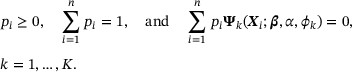
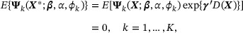
  in the kth subgroup. By double expectation, we have

Note that the second equality holds in the absence of heterogeneity between internal and external studies; that is, the conditional distribution of T given X and the marginal distribution of X are equivalent to their counterparts in the external study. Following Huang et al. (2016), we reexpress the subgroup survival information as a population estimating equation

where  and
and  .
.
In this paper, we apply the empirical likelihood method to integrate information from IPD and the t-year survival probabilities under the semiparametric transformation model. Denote by  the marginal distribution function of X, and by
  the jump size of
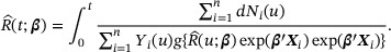
  at the observed data point Xi. We construct the empirical likelihood by multiplying the pseudopartial likelihood and the nonparametric marginal likelihood of X, and then maximize the resulting log-likelihood
subject to the constraints
Note that the constraints were derived from the external information on subgroup survival. Write  and
and  . Applying the classic empirical likelihood argument (Qin & Lawless, 1994; Qin, 2000), we have
  and the constrained log likelihood, up to a constant,
where  are the Lagrange multipliers determined by
  . Hence, we estimate
  by solving the following empirical score functions for zero:
We denote the solution by  . The asymptotic properties of the proposed estimator
  are summarized in Theorem 1, with the proof given in the Supporting Information.
Under regularity conditions for pseudopartial likelihood estimators (Zucker, 2005, p. 1273) and Conditions (S1)∼(S4) stated in the Supporting Information, as  , (i)
, (i)  converges in probability to β0, and (ii)
  converges in distribution to a zero mean multivariate normal distribution with the variance–covariance matrix
  , where
  ,
,  ,
,  , and
, and  .
.
Note that  is semipositive definite because
  is idempotent. As a result, the proposed estimator
  , which combines information from the external study, is asymptotically as or more efficient than the conventional pseudopartial likelihood estimator
  obtained using only the internal study data.
3 Proposed Methods
In practice, the degree of uncertainty in the auxiliary information may not be negligible because the sample size in the external study is not large enough. Moreover, the population and research design usually differ across studies, leading to heterogeneity between internal and external data. This section extends the empirical likelihood method to deal with uncertainty and heterogeneity in the reported t-year survival probabilities.
3.1 Synthesizing External Information with Uncertainty
Suppose that the reported t-year survival probabilities  are estimates of the population parameters
  and were obtained from an external study of N participants. Assume that the asymptotic normality assumption holds for
  , that is,
  approximately follows a multivariate normal distribution with mean zero and variance–covariance matrix V0. To account for uncertainty in the reported t-year survival probabilities, we adopt the augmentation approach proposed in Zhang et al. (2020) by adding an additional normal density term in the empirical likelihood to characterize the contribution of
  and formulating the constraints using the population parameter
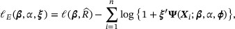
  directly. The augmented log empirical likelihood, up to a constant, is given by
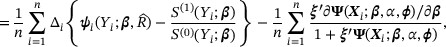
where the last term  reflects variability in the external information. To estimate β, we maximize (17) subject to the constraints
Unlike the empirical likelihood method described in Section 2.2, the constraints are formulated using the population parameter ϕ instead of the value of the AD  .
.
By a standard empirical likelihood argument and argued as in Section 2.2, we can estimate  by maximizing the objective function
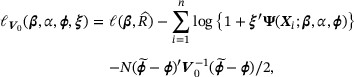
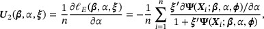
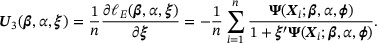
where ξ is the Lagrange multiplier satisfying  . Let
. Let  be the derivative of
  with respect to
  . The maximizer, denoted by
  , can be obtained by solving
  using the Newton–Raphson algorithm. The asymptotic properties of
  are summarized in Theorem 2, with the proof given in the Supporting Information.
Under regularity conditions for pseudopartial likelihood estimators (Zucker, 2005, p. 1273) and Conditions (S1)∼(S4) stated in the Supporting Information, assume that there exists a constant  so that
  . Then, as
  , (i)
, (i)  converges in probability to β0 and (ii)
  converges in distribution to a zero mean multivariate normal distribution with variance–covariance matrix
  , where
  ,
,  , and
, and  .
.
Arguing as in Section 2.2, one can show that  is semipositive definite and hence
  is asymptotically as or more efficient than
  . When
  , that is, the uncertainty in the external information is negligible, it follows from
  that
that  , and thus, the asymptotic variance of
  is close to that of
  . On the other hand, when
  , we have
  , and thus, there is almost no efficiency gain when compared with
  .
.
Intuitively, when V0 is not available from the external source, a consistent estimator of V0 can be obtained using data from the internal study. Since  is asymptotically negligible, the asymptotic variance of the proposed estimator of β remains the same if V0 is replaced by its consistent estimator. However, it is worthwhile to point out that the variance–covariance matrix V0 involves the external censoring time distribution when the censoring time distribution differs between internal and external studies. Without assuming the same distribution on the censoring time, the proposed method explicitly requires that V0 is available from the external source.
3.2 Synthesizing External Information in the Presence of Population Heterogeneity
We now consider the situation where the distribution of covariates in the internal study differs from that in the external study. Denote by  the density functions of X* in the external study and by
  the density functions of X in the internal study. To characterize the differences between
  and
and  , we employ a semiparametric density ratio model

where  is a prespecified q-dimensional function of X, γ is a q-dimensional vector of parameters, and fX(x) is left unspecified. Interestingly, the semiparametric model specified in (20) is equivalent to imposing a (parametric) logistic regression model for membership in the internal (vs. external) study given X. In practice, the selection of covariates involved in D(X) can be informed by comparing the summary statistics of covariates, such as means and variances, which are typically available in the medical reports. For example, if the mean of
  and the variance of X1 (but not X2) are found to be different between internal and external studies, one may specify
  . The parameter γ in (20) characterizes the degree of heterogeneity in the covariate distribution between studies, with
  implying no population heterogeneity.
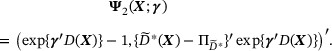
By employing Model (20) to account for the heterogeneity, we can derive a new set of weighted estimating equations
where the weight  reflects the magnitude of heterogeneity. In the absence of heterogeneity, that is,
  , Equation (21) reduces to equation (9). It is worthwhile to point out that imposing the semiparametric density ratio model (20) introduces extra parameters; thus, a direct application of the estimation procedure proposed in the previous sections may encounter identifiability problems. To circumvent this challenge, we seek to exploit information in the covariate summary statistics to construct an additional set of constraints to improve model identification. Based on the summary statistics
  , an additional set of estimating equations for γ can be derived as
  and
and  , where the latter reflects
  . Collectively, we have
  , where
  with
with

In  ,
,  can be different from
  as long as
  satisfies the regular conditions in the Appendix. Moreover, the number of the additional estimating equations for γ can be greater than q.
We proposed to estimate β by maximizing the augmented log empirical likelihood function

subject to the constraints

where the third constraint is the empirical version of the population estimating equation  .
.
Arguing as in Section 2.2, we can estimate  by maximizing the objective function

where ξ is the Lagrange multiplier satisfying  . Let
. Let  be the derivative of
  with respect to
  . The maximizer, denoted by
  , can be obtained by solving
 using the Newton–Raphson algorithm. The asymptotic properties of
  are summarized in Theorem 3, with proof given in the Supporting Information.
Under regularity conditions for pseudopartial likelihood estimators (Zucker, 2005, p. 1273) and Conditions (A1)∼(A4) stated in the Appendix, assume that there exists a constant  so that
  . Then, as
  , (i)
, (i)  converges in probability to β0 and (ii)
  converges in distribution to a zero mean multivariate normal distribution with covariance matrix
  , where
  ,
,  ,
,  ,
,  ,
,  ,
,  ,
,  , and
, and  .
.
It follows from the fact that  is semipositive definite that the proposed estimator
  is asymptotically as or more efficient than the conventional pseudopartial likelihood estimator
  . When
  , we have
  ≈
≈  and thus
  , with
  . In this case, the asymptotic variance–covariance matrix of
  is
is  and is free of V0 as the uncertainty in the external information is negligible. On the other hand, when
  , we have
  , and thus, there is no efficiency gain when compared with
  . Note that
  can be more efficient than
  in the absence of heterogeneity. This is because the efficiency loss resulting from estimating an extra set of parameters in the density ratio model can be compensated by including additional constraints based on the marginal covariate distribution.
4 Numerical Simulations
Simulation studies were conducted to evaluate the performance of the proposed methods under two special cases of the semiparametric transformation model, namely, the Cox model and the proportional odds model. For the internal study, we independently generated X1 from the standard normal distribution N(0, 1) and X2 from the Bernoulli distribution with  . Given
  , the survival time T has a cumulative hazard function
  . We considered two sets of model specifications: (I)
  with
with  and (II)
  with
with  . The follow-up time C was generated from a uniform distribution so that the censoring rate was approximately 30%. In all simulations, 1000 internal study datasets were generated, each with n = 400.
On the other hand, the external study data were generated with or without the homogeneity assumption on the covariate distribution. Specifically, for the homogeneity case, the simulation setting was identical to that of the internal study. For the heterogeneity case,  was generated from the normal distribution with mean 0.2 and variance 0.49, whereas
  was generated from the Bernoulli distribution with
  . Hence, the density ratio model
  , with
  , characterized the difference in the covariate distribution between internal and external studies. All other simulation settings were the same as the internal study. The external study sample size was set to be
  and 400 for different degrees of uncertainty in the external information.
We considered external information in the form of survival probability at  for the two subgroups:
  and
and  . For the homogeneity case, the true survival probabilities of subgroups Ω1 and Ω2 are 0.68 and 0.84 under the Cox model and 0.72 and 0.85 under the proportional odds model; for the heterogeneity case, the subgroup survival probabilities are 0.72 and 0.83 under the Cox model and are 0.75 and 0.84 under the proportional odds model. In each simulation, the subgroup survival probabilities
  ,
,  , were estimated using the Kaplan–Meier method with the external study data, and the variance–covariance matrix V0 was calculated using Greenwood's formula. Finally, when adjusting for heterogeneity via the density ratio model, we also incorporated summary statistics of the covariates in the external study, given in the form of
  with
with  , to improve model estimation.
Tables 1 and 2 summarize the performance of proposed methods under the homogeneity assumption on the covariate distribution, whereas Tables 3 and 4 summarize their performance in the heterogeneity case. We examined the biases, asymptotic standard errors, and empirical standard deviations of the conventional pseudopartial likelihood estimator ( ), the maximum likelihood estimator (MLE,
  ) implemented using the R package transmdl, the empirical likelihood estimator without accounting for uncertainty (
 ), the augmented empirical likelihood estimator accounting for uncertainty but not population heterogeneity (
 ), and the estimator accounting for both uncertainty and heterogeneity by employing a density ratio model (
 ).
).
Summary of simulation results for the Cox model assuming 
| β1 | β2 | β3 | ||||||||||
|---|---|---|---|---|---|---|---|---|---|---|---|---|
| Bias | ESD(ASE) | CP | RE | Bias | ESD(ASE) | CP | RE | Bias | ESD(ASE) | CP | RE | |
Scenario (I):  | ||||||||||||
 | −7 | 64(66) | 95.4 | – | 6 | 124(123) | 94.7 | – | – | – | – | – |
 | −7 | 64(66) | 95.4 | 1.00 | 6 | 124(123) | 94.7 | 1.00 | – | – | – | – |
 | −6 | 26(25) | 94.6 | 6.68 | 5 | 124(123) | 94.2 | 1.01 | – | – | – | – |
| N = 400 | ||||||||||||
 | −8 | 62(63) | 94.8 | 1.07 | 6 | 124(123) | 94.8 | 1.00 | – | – | – | – |
 | −8 | 62(63) | 95.3 | 1.07 | 6 | 124(123) | 94.8 | 1.00 | – | – | – | – |
| N = 10,000 | ||||||||||||
 | −7 | 41(40) | 95.6 | 2.44 | 5 | 124(123) | 94.6 | 1.00 | – | – | – | – |
 | −5 | 39(39) | 94.4 | 2.66 | 5 | 124(123) | 94.7 | 1.00 | – | – | – | – |
Scenario (II):  | ||||||||||||
 | −9 | 97(95) | 94.3 | – | 10 | 129(129) | 95.6 | – | −2 | 132(129) | 93.8 | – |
 | −9 | 97(95) | 94.3 | 1.00 | 10 | 129(129) | 95.6 | 1.00 | −2 | 132(129) | 93.8 | 1.00 |
 | −6 | 27(27) | 94.6 | 12.46 | 9 | 127(127) | 94.9 | 1.03 | −3 | 99(98) | 93.9 | 1.79 |
| N = 400 | ||||||||||||
 | −10 | 90(87) | 94.0 | 1.15 | 10 | 129(128) | 95.4 | 1.00 | 0 | 129(124) | 94.0 | 1.06 |
 | −10 | 90(87) | 94.1 | 1.15 | 10 | 129(128) | 95.4 | 1.00 | 0 | 128(124) | 93.8 | 1.06 |
| N = 10,000 | ||||||||||||
 | −7 | 46(45) | 95.0 | 4.33 | 9 | 128(127) | 94.1 | 1.02 | −2 | 105(103) | 94.7 | 1.60 |
 | −6 | 44(43) | 94.1 | 4.85 | 9 | 127(127) | 95.4 | 1.03 | −3 | 104(103) | 95.2 | 1.63 |
| β1 | β2 | β3 | ||||||||||
|---|---|---|---|---|---|---|---|---|---|---|---|---|
| Bias | ESD(ASE) | CP | RE | Bias | ESD(ASE) | CP | RE | Bias | ESD(ASE) | CP | RE | |
| Scenario (I): | ||||||||||||
| −7 | 64(66) | 95.4 | – | 6 | 124(123) | 94.7 | – | – | – | – | – |
| −7 | 64(66) | 95.4 | 1.00 | 6 | 124(123) | 94.7 | 1.00 | – | – | – | – |
| −6 | 26(25) | 94.6 | 6.68 | 5 | 124(123) | 94.2 | 1.01 | – | – | – | – |
| N = 400 | ||||||||||||
| −8 | 62(63) | 94.8 | 1.07 | 6 | 124(123) | 94.8 | 1.00 | – | – | – | – |
| −8 | 62(63) | 95.3 | 1.07 | 6 | 124(123) | 94.8 | 1.00 | – | – | – | – |
| N = 10,000 | ||||||||||||
| −7 | 41(40) | 95.6 | 2.44 | 5 | 124(123) | 94.6 | 1.00 | – | – | – | – |
| −5 | 39(39) | 94.4 | 2.66 | 5 | 124(123) | 94.7 | 1.00 | – | – | – | – |
| Scenario (II): | ||||||||||||
| −9 | 97(95) | 94.3 | – | 10 | 129(129) | 95.6 | – | −2 | 132(129) | 93.8 | – |
| −9 | 97(95) | 94.3 | 1.00 | 10 | 129(129) | 95.6 | 1.00 | −2 | 132(129) | 93.8 | 1.00 |
| −6 | 27(27) | 94.6 | 12.46 | 9 | 127(127) | 94.9 | 1.03 | −3 | 99(98) | 93.9 | 1.79 |
| N = 400 | ||||||||||||
| −10 | 90(87) | 94.0 | 1.15 | 10 | 129(128) | 95.4 | 1.00 | 0 | 129(124) | 94.0 | 1.06 |
| −10 | 90(87) | 94.1 | 1.15 | 10 | 129(128) | 95.4 | 1.00 | 0 | 128(124) | 93.8 | 1.06 |
| N = 10,000 | ||||||||||||
| −7 | 46(45) | 95.0 | 4.33 | 9 | 128(127) | 94.1 | 1.02 | −2 | 105(103) | 94.7 | 1.60 |
| −6 | 44(43) | 94.1 | 4.85 | 9 | 127(127) | 95.4 | 1.03 | −3 | 104(103) | 95.2 | 1.63 |
Note:  , the pseudopartial likelihood estimator;
  , the maximum likelihood estimator;
  , the empirical likelihood estimator;
  , the proposed estimator accounting for uncertainty in auxiliary information;
  , the proposed estimator accounting for population heterogeneity and uncertainty in auxiliary information. Bias, ESD, ASE, and CP are empirical bias (× 1000), empirical standard deviation (× 1000), the average of the estimated asymptotic standard error (× 1000) over 1000 simulated datasets, and the 95% coverage probability. RE, the empirical variance of
  divided by that of the proposed estimators.
Summary of simulation results for the Cox model assuming
| β1 | β2 | β3 | ||||||||||
|---|---|---|---|---|---|---|---|---|---|---|---|---|
| Bias | ESD(ASE) | CP | RE | Bias | ESD(ASE) | CP | RE | Bias | ESD(ASE) | CP | RE | |
| Scenario (I): | ||||||||||||
| −7 | 64(66) | 95.4 | – | 6 | 124(123) | 94.7 | – | – | – | – | – |
| −7 | 64(66) | 95.4 | 1.00 | 6 | 124(123) | 94.7 | 1.00 | – | – | – | – |
| −6 | 26(25) | 94.6 | 6.68 | 5 | 124(123) | 94.2 | 1.01 | – | – | – | – |
| N = 400 | ||||||||||||
| −8 | 62(63) | 94.8 | 1.07 | 6 | 124(123) | 94.8 | 1.00 | – | – | – | – |
| −8 | 62(63) | 95.3 | 1.07 | 6 | 124(123) | 94.8 | 1.00 | – | – | – | – |
| N = 10,000 | ||||||||||||
| −7 | 41(40) | 95.6 | 2.44 | 5 | 124(123) | 94.6 | 1.00 | – | – | – | – |
| −5 | 39(39) | 94.4 | 2.66 | 5 | 124(123) | 94.7 | 1.00 | – | – | – | – |
| Scenario (II): | ||||||||||||
| −9 | 97(95) | 94.3 | – | 10 | 129(129) | 95.6 | – | −2 | 132(129) | 93.8 | – |
| −9 | 97(95) | 94.3 | 1.00 | 10 | 129(129) | 95.6 | 1.00 | −2 | 132(129) | 93.8 | 1.00 |
| −6 | 27(27) | 94.6 | 12.46 | 9 | 127(127) | 94.9 | 1.03 | −3 | 99(98) | 93.9 | 1.79 |
| N = 400 | ||||||||||||
| −10 | 90(87) | 94.0 | 1.15 | 10 | 129(128) | 95.4 | 1.00 | 0 | 129(124) | 94.0 | 1.06 |
| −10 | 90(87) | 94.1 | 1.15 | 10 | 129(128) | 95.4 | 1.00 | 0 | 128(124) | 93.8 | 1.06 |
| N = 10,000 | ||||||||||||
| −7 | 46(45) | 95.0 | 4.33 | 9 | 128(127) | 94.1 | 1.02 | −2 | 105(103) | 94.7 | 1.60 |
| −6 | 44(43) | 94.1 | 4.85 | 9 | 127(127) | 95.4 | 1.03 | −3 | 104(103) | 95.2 | 1.63 |
Note: , the pseudopartial likelihood estimator; , the maximum likelihood estimator; , the empirical likelihood estimator; , the proposed estimator accounting for uncertainty in auxiliary information; , the proposed estimator accounting for population heterogeneity and uncertainty in auxiliary information. Bias, ESD, ASE, and CP are empirical bias (× 1000), empirical standard deviation (× 1000), the average of the estimated asymptotic standard error (× 1000) over 1000 simulated datasets, and the 95% coverage probability. RE, the empirical variance of divided by that of the proposed estimators.
Summary of simulation results for the proportional odds model assuming 
| β1 | β2 | β3 | ||||||||||
|---|---|---|---|---|---|---|---|---|---|---|---|---|
| Bias | ESD(ASE) | CP | RE | Bias | ESD(ASE) | CP | RE | Bias | ESD(ASE) | CP | RE | |
Scenario (I):  | ||||||||||||
 | −5 | 95(97) | 95.3 | – | 8 | 188(188) | 94.8 | – | – | – | – | – |
 | −6 | 94(96) | 95.5 | 1.01 | −3 | 187(188) | 95.6 | 1.01 | ||||
 | −6 | 28(27) | 95.1 | 13.19 | 9 | 188(188) | 94.8 | 1.01 | – | – | – | – |
| N = 400 | ||||||||||||
 | −9 | 89(90) | 95.7 | 1.14 | 10 | 189(188) | 94.9 | 0.99 | – | – | – | – |
 | −9 | 89(90) | 95.8 | 1.15 | 10 | 189(188) | 94.9 | 0.99 | – | – | – | – |
| N = 10,000 | ||||||||||||
 | −5 | 49(49) | 94.8 | 3.80 | 9 | 189(188) | 94.8 | 1.00 | – | – | – | – |
 | −3 | 47(47) | 94.8 | 4.21 | 9 | 188(188) | 94.8 | 1.00 | – | – | – | – |
Scenario (II):  | ||||||||||||
 | −1 | 139(137) | 94.0 | – | 9 | 193(192) | 94.3 | – | −9 | 193(191) | 94.9 | – |
 | −4 | 137(137) | 94.6 | 1.02 | 7 | 193(192) | 94.7 | 1.01 | 5 | 193(191) | 95.2 | 1.01 |
 | −6 | 28(27) | 94.7 | 24.07 | 9 | 193(191) | 94.4 | 1.01 | −10 | 145(142) | 95.0 | 1.79 |
| N = 400 | ||||||||||||
 | −7 | 122(120) | 95.0 | 1.31 | 13 | 194(192) | 94.1 | 0.99 | −10 | 184(180) | 94.7 | 1.11 |
 | −7 | 121(120) | 95.1 | 1.31 | 13 | 194(192) | 94.2 | 0.99 | −10 | 184(180) | 94.6 | 1.11 |
| N = 10,000 | ||||||||||||
 | −4 | 53(52) | 94.5 | 6.91 | 11 | 193(191) | 94.4 | 1.01 | −12 | 151(148) | 94.6 | 1.64 |
 | −3 | 50(50) | 94.6 | 7.66 | 11 | 193(191) | 94.4 | 1.01 | −13 | 151(147) | 94.4 | 1.64 |
| β1 | β2 | β3 | ||||||||||
|---|---|---|---|---|---|---|---|---|---|---|---|---|
| Bias | ESD(ASE) | CP | RE | Bias | ESD(ASE) | CP | RE | Bias | ESD(ASE) | CP | RE | |
| Scenario (I): | ||||||||||||
| −5 | 95(97) | 95.3 | – | 8 | 188(188) | 94.8 | – | – | – | – | – |
| −6 | 94(96) | 95.5 | 1.01 | −3 | 187(188) | 95.6 | 1.01 | ||||
| −6 | 28(27) | 95.1 | 13.19 | 9 | 188(188) | 94.8 | 1.01 | – | – | – | – |
| N = 400 | ||||||||||||
| −9 | 89(90) | 95.7 | 1.14 | 10 | 189(188) | 94.9 | 0.99 | – | – | – | – |
| −9 | 89(90) | 95.8 | 1.15 | 10 | 189(188) | 94.9 | 0.99 | – | – | – | – |
| N = 10,000 | ||||||||||||
| −5 | 49(49) | 94.8 | 3.80 | 9 | 189(188) | 94.8 | 1.00 | – | – | – | – |
| −3 | 47(47) | 94.8 | 4.21 | 9 | 188(188) | 94.8 | 1.00 | – | – | – | – |
| Scenario (II): | ||||||||||||
| −1 | 139(137) | 94.0 | – | 9 | 193(192) | 94.3 | – | −9 | 193(191) | 94.9 | – |
| −4 | 137(137) | 94.6 | 1.02 | 7 | 193(192) | 94.7 | 1.01 | 5 | 193(191) | 95.2 | 1.01 |
| −6 | 28(27) | 94.7 | 24.07 | 9 | 193(191) | 94.4 | 1.01 | −10 | 145(142) | 95.0 | 1.79 |
| N = 400 | ||||||||||||
| −7 | 122(120) | 95.0 | 1.31 | 13 | 194(192) | 94.1 | 0.99 | −10 | 184(180) | 94.7 | 1.11 |
| −7 | 121(120) | 95.1 | 1.31 | 13 | 194(192) | 94.2 | 0.99 | −10 | 184(180) | 94.6 | 1.11 |
| N = 10,000 | ||||||||||||
| −4 | 53(52) | 94.5 | 6.91 | 11 | 193(191) | 94.4 | 1.01 | −12 | 151(148) | 94.6 | 1.64 |
| −3 | 50(50) | 94.6 | 7.66 | 11 | 193(191) | 94.4 | 1.01 | −13 | 151(147) | 94.4 | 1.64 |
Note:  , the pseudopartial likelihood estimator;
  , the maximum likelihood estimator;
  , the empirical likelihood estimator;
  , the proposed estimator accounting for uncertainty in auxiliary information;
  , the proposed estimator accounting for population heterogeneity and uncertainty in auxiliary information. Bias, ESD, ASE, and CP are empirical bias (× 1000), empirical standard deviation (× 1000), the average of the estimated asymptotic standard error (× 1000) over 1000 simulated datasets, and the 95% coverage probability. RE, the empirical variance of
  divided by that of the proposed estimators.
Summary of simulation results for the proportional odds model assuming
| β1 | β2 | β3 | ||||||||||
|---|---|---|---|---|---|---|---|---|---|---|---|---|
| Bias | ESD(ASE) | CP | RE | Bias | ESD(ASE) | CP | RE | Bias | ESD(ASE) | CP | RE | |
| Scenario (I): | ||||||||||||
| −5 | 95(97) | 95.3 | – | 8 | 188(188) | 94.8 | – | – | – | – | – |
| −6 | 94(96) | 95.5 | 1.01 | −3 | 187(188) | 95.6 | 1.01 | ||||
| −6 | 28(27) | 95.1 | 13.19 | 9 | 188(188) | 94.8 | 1.01 | – | – | – | – |
| N = 400 | ||||||||||||
| −9 | 89(90) | 95.7 | 1.14 | 10 | 189(188) | 94.9 | 0.99 | – | – | – | – |
| −9 | 89(90) | 95.8 | 1.15 | 10 | 189(188) | 94.9 | 0.99 | – | – | – | – |
| N = 10,000 | ||||||||||||
| −5 | 49(49) | 94.8 | 3.80 | 9 | 189(188) | 94.8 | 1.00 | – | – | – | – |
| −3 | 47(47) | 94.8 | 4.21 | 9 | 188(188) | 94.8 | 1.00 | – | – | – | – |
| Scenario (II): | ||||||||||||
| −1 | 139(137) | 94.0 | – | 9 | 193(192) | 94.3 | – | −9 | 193(191) | 94.9 | – |
| −4 | 137(137) | 94.6 | 1.02 | 7 | 193(192) | 94.7 | 1.01 | 5 | 193(191) | 95.2 | 1.01 |
| −6 | 28(27) | 94.7 | 24.07 | 9 | 193(191) | 94.4 | 1.01 | −10 | 145(142) | 95.0 | 1.79 |
| N = 400 | ||||||||||||
| −7 | 122(120) | 95.0 | 1.31 | 13 | 194(192) | 94.1 | 0.99 | −10 | 184(180) | 94.7 | 1.11 |
| −7 | 121(120) | 95.1 | 1.31 | 13 | 194(192) | 94.2 | 0.99 | −10 | 184(180) | 94.6 | 1.11 |
| N = 10,000 | ||||||||||||
| −4 | 53(52) | 94.5 | 6.91 | 11 | 193(191) | 94.4 | 1.01 | −12 | 151(148) | 94.6 | 1.64 |
| −3 | 50(50) | 94.6 | 7.66 | 11 | 193(191) | 94.4 | 1.01 | −13 | 151(147) | 94.4 | 1.64 |
Note: , the pseudopartial likelihood estimator; , the maximum likelihood estimator; , the empirical likelihood estimator; , the proposed estimator accounting for uncertainty in auxiliary information; , the proposed estimator accounting for population heterogeneity and uncertainty in auxiliary information. Bias, ESD, ASE, and CP are empirical bias (× 1000), empirical standard deviation (× 1000), the average of the estimated asymptotic standard error (× 1000) over 1000 simulated datasets, and the 95% coverage probability. RE, the empirical variance of divided by that of the proposed estimators.
Summary of simulation results for the Cox model assuming 
| β1 | β2 | β3 | ||||||||||
|---|---|---|---|---|---|---|---|---|---|---|---|---|
| Bias | ESD(ASE) | CP | RE | Bias | ESD(ASE) | CP | RE | Bias | ESD(ASE) | CP | RE | |
Scenario (I):  | ||||||||||||
 | −7 | 64(66) | 95.4 | – | 6 | 124(123) | 94.7 | – | – | – | – | – |
 | −7 | 64(66) | 95.4 | 1.00 | 6 | 124(123) | 94.7 | 1.00 | – | – | – | – |
 | 128 | 20(19) | 0 | 10.01 | −15 | 120(123) | 95.5 | 1.07 | – | – | – | – |
| N = 400 | ||||||||||||
 | 8 | 62(62) | 94.7 | 1.08 | 4 | 124(123) | 94.8 | 1.01 | – | – | – | – |
 | −6 | 62(64) | 95.3 | 1.07 | 6 | 124(123) | 94.8 | 1.00 | – | – | – | – |
| N = 10,000 | ||||||||||||
 | 99 | 38(36) | 24.2 | 2.85 | −10 | 120(123) | 95.6 | 1.07 | – | – | – | – |
 | −2 | 42(42) | 92.7 | 2.37 | 5 | 124(123) | 94.6 | 1.01 | – | – | – | – |
 | ||||||||||||
 | −9 | 97(95) | 94.3 | – | 10 | 129(129) | 95.6 | – | −2 | 132(129) | 93.8 | – |
 | −9 | 97(95) | 94.3 | 1.00 | 10 | 129(129) | 95.6 | 1.00 | −2 | 132(129) | 93.8 | 1.00 |
 | 134 | 20(19) | 0 | 23.34 | −14 | 125(127) | 95.3 | 1.06 | −132 | 96(96) | 73.4 | 1.90 |
| N = 400 | ||||||||||||
 | 20 | 89(85) | 92.7 | 1.19 | 4 | 128(128) | 95.3 | 1.02 | −27 | 127(123) | 93.0 | 1.08 |
 | -9 | 93(89) | 93.8 | 1.09 | 10 | 129(128) | 95.2 | 1.01 | −2 | 130(125) | 94.4 | 1.04 |
| N = 10,000 | ||||||||||||
 | 119 | 40(39) | 15.0 | 5.81 | −12 | 125(127) | 95.7 | 1.06 | −118 | 101(101) | 80.1 | 1.73 |
 | −4 | 49(48) | 94.6 | 3.85 | 9 | 127(127) | 95.4 | 1.03 | −5 | 105(105) | 94.5 | 1.60 |
| β1 | β2 | β3 | ||||||||||
|---|---|---|---|---|---|---|---|---|---|---|---|---|
| Bias | ESD(ASE) | CP | RE | Bias | ESD(ASE) | CP | RE | Bias | ESD(ASE) | CP | RE | |
| Scenario (I): | ||||||||||||
| −7 | 64(66) | 95.4 | – | 6 | 124(123) | 94.7 | – | – | – | – | – |
| −7 | 64(66) | 95.4 | 1.00 | 6 | 124(123) | 94.7 | 1.00 | – | – | – | – |
| 128 | 20(19) | 0 | 10.01 | −15 | 120(123) | 95.5 | 1.07 | – | – | – | – |
| N = 400 | ||||||||||||
| 8 | 62(62) | 94.7 | 1.08 | 4 | 124(123) | 94.8 | 1.01 | – | – | – | – |
| −6 | 62(64) | 95.3 | 1.07 | 6 | 124(123) | 94.8 | 1.00 | – | – | – | – |
| N = 10,000 | ||||||||||||
| 99 | 38(36) | 24.2 | 2.85 | −10 | 120(123) | 95.6 | 1.07 | – | – | – | – |
| −2 | 42(42) | 92.7 | 2.37 | 5 | 124(123) | 94.6 | 1.01 | – | – | – | – |
| ||||||||||||
| −9 | 97(95) | 94.3 | – | 10 | 129(129) | 95.6 | – | −2 | 132(129) | 93.8 | – |
| −9 | 97(95) | 94.3 | 1.00 | 10 | 129(129) | 95.6 | 1.00 | −2 | 132(129) | 93.8 | 1.00 |
| 134 | 20(19) | 0 | 23.34 | −14 | 125(127) | 95.3 | 1.06 | −132 | 96(96) | 73.4 | 1.90 |
| N = 400 | ||||||||||||
| 20 | 89(85) | 92.7 | 1.19 | 4 | 128(128) | 95.3 | 1.02 | −27 | 127(123) | 93.0 | 1.08 |
| -9 | 93(89) | 93.8 | 1.09 | 10 | 129(128) | 95.2 | 1.01 | −2 | 130(125) | 94.4 | 1.04 |
| N = 10,000 | ||||||||||||
| 119 | 40(39) | 15.0 | 5.81 | −12 | 125(127) | 95.7 | 1.06 | −118 | 101(101) | 80.1 | 1.73 |
| −4 | 49(48) | 94.6 | 3.85 | 9 | 127(127) | 95.4 | 1.03 | −5 | 105(105) | 94.5 | 1.60 |
Note:  , the pseudopartial likelihood estimator;
  , the maximum likelihood estimator;
  , the empirical likelihood estimator;
  , the proposed estimator accounting for uncertainty in auxiliary information;
  , the proposed estimator accounting for population heterogeneity and uncertainty in auxiliary information. Bias, ESD, ASE, and CP are empirical bias (× 1000), empirical standard deviation (× 1000), the average of the estimated asymptotic standard error (× 1000) over 1000 simulated datasets, and the 95% coverage probability. RE, the empirical variance of
  divided by that of the proposed estimators.
Summary of simulation results for the Cox model assuming
| β1 | β2 | β3 | ||||||||||
|---|---|---|---|---|---|---|---|---|---|---|---|---|
| Bias | ESD(ASE) | CP | RE | Bias | ESD(ASE) | CP | RE | Bias | ESD(ASE) | CP | RE | |
| Scenario (I): | ||||||||||||
| −7 | 64(66) | 95.4 | – | 6 | 124(123) | 94.7 | – | – | – | – | – |
| −7 | 64(66) | 95.4 | 1.00 | 6 | 124(123) | 94.7 | 1.00 | – | – | – | – |
| 128 | 20(19) | 0 | 10.01 | −15 | 120(123) | 95.5 | 1.07 | – | – | – | – |
| N = 400 | ||||||||||||
| 8 | 62(62) | 94.7 | 1.08 | 4 | 124(123) | 94.8 | 1.01 | – | – | – | – |
| −6 | 62(64) | 95.3 | 1.07 | 6 | 124(123) | 94.8 | 1.00 | – | – | – | – |
| N = 10,000 | ||||||||||||
| 99 | 38(36) | 24.2 | 2.85 | −10 | 120(123) | 95.6 | 1.07 | – | – | – | – |
| −2 | 42(42) | 92.7 | 2.37 | 5 | 124(123) | 94.6 | 1.01 | – | – | – | – |
| ||||||||||||
| −9 | 97(95) | 94.3 | – | 10 | 129(129) | 95.6 | – | −2 | 132(129) | 93.8 | – |
| −9 | 97(95) | 94.3 | 1.00 | 10 | 129(129) | 95.6 | 1.00 | −2 | 132(129) | 93.8 | 1.00 |
| 134 | 20(19) | 0 | 23.34 | −14 | 125(127) | 95.3 | 1.06 | −132 | 96(96) | 73.4 | 1.90 |
| N = 400 | ||||||||||||
| 20 | 89(85) | 92.7 | 1.19 | 4 | 128(128) | 95.3 | 1.02 | −27 | 127(123) | 93.0 | 1.08 |
| -9 | 93(89) | 93.8 | 1.09 | 10 | 129(128) | 95.2 | 1.01 | −2 | 130(125) | 94.4 | 1.04 |
| N = 10,000 | ||||||||||||
| 119 | 40(39) | 15.0 | 5.81 | −12 | 125(127) | 95.7 | 1.06 | −118 | 101(101) | 80.1 | 1.73 |
| −4 | 49(48) | 94.6 | 3.85 | 9 | 127(127) | 95.4 | 1.03 | −5 | 105(105) | 94.5 | 1.60 |
Note: , the pseudopartial likelihood estimator; , the maximum likelihood estimator; , the empirical likelihood estimator; , the proposed estimator accounting for uncertainty in auxiliary information; , the proposed estimator accounting for population heterogeneity and uncertainty in auxiliary information. Bias, ESD, ASE, and CP are empirical bias (× 1000), empirical standard deviation (× 1000), the average of the estimated asymptotic standard error (× 1000) over 1000 simulated datasets, and the 95% coverage probability. RE, the empirical variance of divided by that of the proposed estimators.
Summary of simulation results for the proportional odds model assuming 
| β1 | β2 | β3 | ||||||||||
|---|---|---|---|---|---|---|---|---|---|---|---|---|
| Bias | ESD(ASE) | CP | RE | Bias | ESD(ASE) | CP | RE | Bias | ESD(ASE) | CP | RE | |
Scenario (I):  | ||||||||||||
 | −5 | 95(97) | 95.3 | – | 8 | 188(188) | 94.8 | – | – | – | – | – |
 | −6 | 94(96) | 95.5 | 1.01 | −3 | 187(188) | 95.6 | 1.01 | ||||
 | 138 | 20(19) | 0 | 22.31 | 1 | 185(188) | 95.2 | 1.03 | – | – | – | – |
| N = 400 | ||||||||||||
 | 16 | 89(89) | 93.8 | 1.15 | 8 | 188(188) | 94.7 | 1.00 | – | – | – | – |
 | −7 | 91(92) | 93.9 | 1.09 | 10 | 189(188) | 94.8 | 0.99 | – | – | – | – |
| N = 10,000 | ||||||||||||
 | 117 | 44(43) | 24.1 | 4.68 | 2 | 186(188) | 95.0 | 1.03 | – | – | – | – |
 | −3 | 54(53) | 95.0 | 3.17 | 9 | 188(188) | 94.9 | 1.00 | – | – | – | – |
Scenario (II):  | ||||||||||||
 | −1 | 139(137) | 94.0 | − | 9 | 193(192) | 94.3 | – | −9 | 193(191) | 94.9 | – |
 | −4 | 137(137) | 94.6 | 1.02 | 7 | 193(192) | 94.7 | 1.01 | 5 | 193(191) | 95.2 | 1.01 |
 | 141 | 20(19) | 0 | 48.02 | 0 | 191(191) | 94.0 | 1.02 | −152 | 143(140) | 81.2 | 1.84 |
| N = 400 | ||||||||||||
 | 36 | 119(117) | 93.7 | 1.36 | 10 | 194(192) | 94.3 | 1.00 | −52 | 181(178) | 94.0 | 1.14 |
 | −3 | 127(125) | 95.1 | 1.19 | 13 | 194(192) | 94.2 | 0.99 | −14 | 186(183) | 94.7 | 1.08 |
| N = 10,000 | ||||||||||||
 | 132 | 46(45) | 18.3 | 9.21 | 1 | 191(191) | 94.2 | 1.02 | −143 | 148(146) | 83.8 | 1.71 |
 | 1 | 57(58) | 95.3 | 5.88 | 11 | 193(191) | 94.2 | 1.00 | −17 | 153(150) | 94.3 | 1.60 |
| β1 | β2 | β3 | ||||||||||
|---|---|---|---|---|---|---|---|---|---|---|---|---|
| Bias | ESD(ASE) | CP | RE | Bias | ESD(ASE) | CP | RE | Bias | ESD(ASE) | CP | RE | |
| Scenario (I): | ||||||||||||
| −5 | 95(97) | 95.3 | – | 8 | 188(188) | 94.8 | – | – | – | – | – |
| −6 | 94(96) | 95.5 | 1.01 | −3 | 187(188) | 95.6 | 1.01 | ||||
| 138 | 20(19) | 0 | 22.31 | 1 | 185(188) | 95.2 | 1.03 | – | – | – | – |
| N = 400 | ||||||||||||
| 16 | 89(89) | 93.8 | 1.15 | 8 | 188(188) | 94.7 | 1.00 | – | – | – | – |
| −7 | 91(92) | 93.9 | 1.09 | 10 | 189(188) | 94.8 | 0.99 | – | – | – | – |
| N = 10,000 | ||||||||||||
| 117 | 44(43) | 24.1 | 4.68 | 2 | 186(188) | 95.0 | 1.03 | – | – | – | – |
| −3 | 54(53) | 95.0 | 3.17 | 9 | 188(188) | 94.9 | 1.00 | – | – | – | – |
| Scenario (II): | ||||||||||||
| −1 | 139(137) | 94.0 | − | 9 | 193(192) | 94.3 | – | −9 | 193(191) | 94.9 | – |
| −4 | 137(137) | 94.6 | 1.02 | 7 | 193(192) | 94.7 | 1.01 | 5 | 193(191) | 95.2 | 1.01 |
| 141 | 20(19) | 0 | 48.02 | 0 | 191(191) | 94.0 | 1.02 | −152 | 143(140) | 81.2 | 1.84 |
| N = 400 | ||||||||||||
| 36 | 119(117) | 93.7 | 1.36 | 10 | 194(192) | 94.3 | 1.00 | −52 | 181(178) | 94.0 | 1.14 |
| −3 | 127(125) | 95.1 | 1.19 | 13 | 194(192) | 94.2 | 0.99 | −14 | 186(183) | 94.7 | 1.08 |
| N = 10,000 | ||||||||||||
| 132 | 46(45) | 18.3 | 9.21 | 1 | 191(191) | 94.2 | 1.02 | −143 | 148(146) | 83.8 | 1.71 |
| 1 | 57(58) | 95.3 | 5.88 | 11 | 193(191) | 94.2 | 1.00 | −17 | 153(150) | 94.3 | 1.60 |
Note:  , the pseudopartial likelihood estimator;
  , the maximum likelihood estimator;
  , the empirical likelihood estimator;
  , the proposed estimator accounting for uncertainty in auxiliary information;
  , the proposed estimator accounting for population heterogeneity and uncertainty in auxiliary information. Bias, ESD, ASE, and CP are empirical bias (× 1000), empirical standard deviation (× 1000), the average of the estimated asymptotic standard error (× 1000) over 1000 simulated datasets, and the 95% coverage probability. RE, the empirical variance of
  divided by that of the proposed estimators.
Summary of simulation results for the proportional odds model assuming
| β1 | β2 | β3 | ||||||||||
|---|---|---|---|---|---|---|---|---|---|---|---|---|
| Bias | ESD(ASE) | CP | RE | Bias | ESD(ASE) | CP | RE | Bias | ESD(ASE) | CP | RE | |
| Scenario (I): | ||||||||||||
| −5 | 95(97) | 95.3 | – | 8 | 188(188) | 94.8 | – | – | – | – | – |
| −6 | 94(96) | 95.5 | 1.01 | −3 | 187(188) | 95.6 | 1.01 | ||||
| 138 | 20(19) | 0 | 22.31 | 1 | 185(188) | 95.2 | 1.03 | – | – | – | – |
| N = 400 | ||||||||||||
| 16 | 89(89) | 93.8 | 1.15 | 8 | 188(188) | 94.7 | 1.00 | – | – | – | – |
| −7 | 91(92) | 93.9 | 1.09 | 10 | 189(188) | 94.8 | 0.99 | – | – | – | – |
| N = 10,000 | ||||||||||||
| 117 | 44(43) | 24.1 | 4.68 | 2 | 186(188) | 95.0 | 1.03 | – | – | – | – |
| −3 | 54(53) | 95.0 | 3.17 | 9 | 188(188) | 94.9 | 1.00 | – | – | – | – |
| Scenario (II): | ||||||||||||
| −1 | 139(137) | 94.0 | − | 9 | 193(192) | 94.3 | – | −9 | 193(191) | 94.9 | – |
| −4 | 137(137) | 94.6 | 1.02 | 7 | 193(192) | 94.7 | 1.01 | 5 | 193(191) | 95.2 | 1.01 |
| 141 | 20(19) | 0 | 48.02 | 0 | 191(191) | 94.0 | 1.02 | −152 | 143(140) | 81.2 | 1.84 |
| N = 400 | ||||||||||||
| 36 | 119(117) | 93.7 | 1.36 | 10 | 194(192) | 94.3 | 1.00 | −52 | 181(178) | 94.0 | 1.14 |
| −3 | 127(125) | 95.1 | 1.19 | 13 | 194(192) | 94.2 | 0.99 | −14 | 186(183) | 94.7 | 1.08 |
| N = 10,000 | ||||||||||||
| 132 | 46(45) | 18.3 | 9.21 | 1 | 191(191) | 94.2 | 1.02 | −143 | 148(146) | 83.8 | 1.71 |
| 1 | 57(58) | 95.3 | 5.88 | 11 | 193(191) | 94.2 | 1.00 | −17 | 153(150) | 94.3 | 1.60 |
Note: , the pseudopartial likelihood estimator; , the maximum likelihood estimator; , the empirical likelihood estimator; , the proposed estimator accounting for uncertainty in auxiliary information; , the proposed estimator accounting for population heterogeneity and uncertainty in auxiliary information. Bias, ESD, ASE, and CP are empirical bias (× 1000), empirical standard deviation (× 1000), the average of the estimated asymptotic standard error (× 1000) over 1000 simulated datasets, and the 95% coverage probability. RE, the empirical variance of divided by that of the proposed estimators.
In the absence of population heterogeneity, all methods yield a small bias in the parameter estimation and the coverage rates of the 95% confidence intervals based on the estimated asymptotic standard errors are very close to the nominal level (0.95). Compared with  , the proposed methods enjoy efficiency gains in estimating β1 in Scenario (I) and both β1 and β3 in Scenario (II) with the upper bound given by that of
  , but not β2 in either case. Note that the external information consists of two exclusive subgroups differed by their values in X1 but not X2. Thus, the efficiency gain is mainly observed for effects involving X1. On the other hand,
  is slightly more efficient than
  , with the relative efficiency ranging from 1.01 to 1.02. Yet, it is computationally more costly than its competitors. The computation burden of the MLE is 52 times higher than that of
  (26,382 s vs. 509 s for analyzing 10 datasets with
  and
and  ).
).
When heterogeneity between internal and external studies is present, Table 3 and 4 show that  and
and  , the augmented empirical likelihood estimators without accounting for heterogeneity, can yield large biases. When a density ratio model is employed to characterize population heterogeneity,
  yields small biases while enjoying efficiency gains under all scenarios. When information from a large external study with
  was exploited, the relative efficiency in estimating β1 under Scenario (I) is 2.19 and 3.28 for the Cox model and the proportional odds model, respectively. On the other hand, the relative efficiency in Scenario (II) can be as high as 3.86 and 1.59 in estimating β1 and β3 under the Cox model, and 5.87 and 1.60 under the proportional odds model.
To investigate the robustness of the proposed methods against model misspecification, we carried out additional simulation studies with incorrect choices of  in the semiparametric density ratio model. The results are presented in Tables S1–S2 of the Supporting Information. In the case where
  fails to include X2, the bias in estimating β remains negligible, and the efficiency gain is similar to that under the correctly specified model. On the other hand, failing to include X1 or
  in
in  leads to larger biases in parameter estimation. The results can be explained by the fact that the external information consists of two exclusive subgroups differed by their values in X1 but not in X2. Thus model misspecification has a minor impact on the estimation of β when X2 is not included in
  .
.
Following the suggestions of the reviewers, we expanded simulation studies by including the smaller internal sample sizes  and 200, varying the external sample size N from 200 to 10,000, and considered different censoring rates. The results show that the proposed methods perform well in all situations. Details of additional simulation studies are reported in Section S2 of the Supporting Information. Moreover, since
  may not be available in practice, we studied the asymptotic properties and investigated numerical performance of the proposed method when its estimate
  is employed instead. As expected, replacing
  with its estimate yields a larger asymptotic variance. Interestingly, simulation studies show that two estimators have a similar numerical performance in estimating β but not γ. Details can be found in Section 3 of the Supplementary Information.
5 Pancreatic Cancer Data Analysis
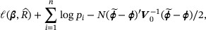
Pancreatic cancer is a highly aggressive disease. According to Global Cancer Statistics 2020 (Sung et al., 2021), pancreatic cancer is the seventh leading cause of cancer death in the world, and its incidence rate is on the rise. Late diagnosis, early metastasis, and lack of effective therapy have contributed to the dismal overall prognosis, with only 6% of the patients surviving more than 5 years after diagnosis. Despite recent advances in cancer diagnosis and treatment, surgical resection remains the only possible curative option for pancreatic cancer. However, less than 20% of the patients are eligible for resection when diagnosed, as they often present at advanced stages. Moreover, most patients with resectable pancreatic cancer have an unfavorable outcome due to recurrent disease within a few years. The 5-year survival probability after resection is reported to be around 34.5% (Yamamoto et al., 2015). Hence, it is crucial to identify prognostic factors for pancreatic cancer patients to improve disease management.
In the Johns Hopkins Hospital pancreatic cancer study described in Section 1, patients' demographic information, treatments, and clinical and pathological exam were collected via a retrospective chart review. All-cause and cancer-specific deaths were determined by a combined review of clinical information, Social Security Death Index, and the National Cancer Database. Prognostic factors of interest in our analysis included resection margin status, lymph node involvement, invasion of the surrounding nerves, age, and gender. After excluding patients with missing data, the mean age at the time of surgery among the 204 remaining patients was 64.2 years. About half of the patients were male (51.9%) and had positive resection margins (48.0%). The majority of the patients had perineural invasion (PNI) (94.1%) and lymph node involvement (86.2%).
To evaluate the effects of prognostic factors on survival after pancreatectomy, we fit two special cases of the semiparametric transformation model: the Cox model and the proportional odds model. As reported in Table 5, both sets of analysis concluded that female sex, older age, PNI, node positivity, and margin positivity were associated with poorer prognosis. However, the effect of node status, a known prognostic factor, did not reach statistical significance in both models, most likely due to the small sample size of patients without lymph node involvement.
Estimated regression coefficients of the Cox model and the proportional odds model for the pancreatic cancer study
| Node positive | Margin positive | PNI | >65 years | Male | γ0 | γ1 | γ2 | |||||||||
|---|---|---|---|---|---|---|---|---|---|---|---|---|---|---|---|---|
| Est | SE | Est | SE | Est | SE | Est | SE | Est | SE | Est | SE | Est | SE | Est | SE | |
| Cox model | ||||||||||||||||
 | 0.363 | 0.226 | 0.407 | 0.153 | 1.124 | 0.373 | 0.282 | 0.153 | −0.295 | 0.154 | – | – | – | – | – | – |
 | 0.509 | 0.158 | 0.393 | 0.153 | 1.128 | 0.373 | 0.275 | 0.153 | −0.291 | 0.154 | 1.141 | 0.226 | −0.867 | 0.269 | −1.098 | 0.290 |
| Proportional odds model | ||||||||||||||||
 | 0.654 | 0.373 | 0.916 | 0.256 | 2.096 | 0.744 | 0.385 | 0.246 | −0.341 | 0.248 | – | – | – | – | – | – |
 | 0.877 | 0.282 | 0.899 | 0.255 | 2.089 | 0.743 | 0.377 | 0.245 | −0.340 | 0.249 | 1.143 | 0.226 | −0.867 | 0.269 | −1.100 | 0.290 |
| Node positive | Margin positive | PNI | >65 years | Male | γ0 | γ1 | γ2 | |||||||||
|---|---|---|---|---|---|---|---|---|---|---|---|---|---|---|---|---|
| Est | SE | Est | SE | Est | SE | Est | SE | Est | SE | Est | SE | Est | SE | Est | SE | |
| Cox model | ||||||||||||||||
| 0.363 | 0.226 | 0.407 | 0.153 | 1.124 | 0.373 | 0.282 | 0.153 | −0.295 | 0.154 | – | – | – | – | – | – |
| 0.509 | 0.158 | 0.393 | 0.153 | 1.128 | 0.373 | 0.275 | 0.153 | −0.291 | 0.154 | 1.141 | 0.226 | −0.867 | 0.269 | −1.098 | 0.290 |
| Proportional odds model | ||||||||||||||||
| 0.654 | 0.373 | 0.916 | 0.256 | 2.096 | 0.744 | 0.385 | 0.246 | −0.341 | 0.248 | – | – | – | – | – | – |
| 0.877 | 0.282 | 0.899 | 0.255 | 2.089 | 0.743 | 0.377 | 0.245 | −0.340 | 0.249 | 1.143 | 0.226 | −0.867 | 0.269 | −1.100 | 0.290 |
Note:  , the conventional pseudopartial likelihood estimator without synthesizing auxiliary information;
  , the proposed estimator accounting for uncertainty and heterogeneity in the external information. Est denotes the estimate, SE denotes the standard error, which is calculated by the square root of the asymptotic variance.
  , and γ2, the regression parameters of the density ratio model corresponding to intercept, margin positivity, and node positivity, respectively.
Estimated regression coefficients of the Cox model and the proportional odds model for the pancreatic cancer study
| Node positive | Margin positive | PNI | >65 years | Male | γ0 | γ1 | γ2 | |||||||||
|---|---|---|---|---|---|---|---|---|---|---|---|---|---|---|---|---|
| Est | SE | Est | SE | Est | SE | Est | SE | Est | SE | Est | SE | Est | SE | Est | SE | |
| Cox model | ||||||||||||||||
| 0.363 | 0.226 | 0.407 | 0.153 | 1.124 | 0.373 | 0.282 | 0.153 | −0.295 | 0.154 | – | – | – | – | – | – |
| 0.509 | 0.158 | 0.393 | 0.153 | 1.128 | 0.373 | 0.275 | 0.153 | −0.291 | 0.154 | 1.141 | 0.226 | −0.867 | 0.269 | −1.098 | 0.290 |
| Proportional odds model | ||||||||||||||||
| 0.654 | 0.373 | 0.916 | 0.256 | 2.096 | 0.744 | 0.385 | 0.246 | −0.341 | 0.248 | – | – | – | – | – | – |
| 0.877 | 0.282 | 0.899 | 0.255 | 2.089 | 0.743 | 0.377 | 0.245 | −0.340 | 0.249 | 1.143 | 0.226 | −0.867 | 0.269 | −1.100 | 0.290 |
Note: , the conventional pseudopartial likelihood estimator without synthesizing auxiliary information; , the proposed estimator accounting for uncertainty and heterogeneity in the external information. Est denotes the estimate, SE denotes the standard error, which is calculated by the square root of the asymptotic variance. , and γ2, the regression parameters of the density ratio model corresponding to intercept, margin positivity, and node positivity, respectively.
To improve estimation efficiency, we seek to incorporate information from Ahmad et al. (2001), which reported 3-year survival probabilities with respect to lymph node status based on data from 116 patients. From this study, we exploited two sets of 3-year subgroup survival probabilities: 14% for patients with positive node status and 38% for patients with negative node status. An examination of the available covariate summary statistics revealed that the proportions of margin-positive and node-positive patients in the external study were only 24% and 62%, respectively, which were much lower than that in the internal study (48% and 86%, respectively), indicating strong heterogeneity between the covariate distributions between the internal and external study. As discussed in Section 3.2, we constructed a density ratio model with margin status and node status to account for the heterogeneity between the covariate distributions. Note that we applied the estimator described in Section 3 of the Supporting Information to account for variability in the covariate summary statistics.
Table 5 summarizes the fitted Cox model and the fitted proportional odds model using the proposed methods. We extracted the standard errors of the reported 3-year survival probabilities from Ahmad et al. (2001) to evaluate the degree of uncertainty in the external information. In particular, a significant efficiency gain is observed in estimating the effects of node positivity, which determined the two subgroups in the external information. The estimated coefficients of margin positivity and node positivity in the density ratio model are −0.867 (95% CI, [ 0.340]) and −1.098 (95% CI, [
 0.529]), respectively, under the Cox model, and −0.867 (95% CI, [
 0.339]) and −1.100 (95% CI, [
 0.531]), respectively, under the proportional odds model, indicating significant heterogeneity between internal and external studies. Interestingly, the efficiency loss due to estimating an additional set of parameters in the density ratio model is minimal. As a result, compared with
  , the relative efficiency in estimating node positivity is 2.046 under the Cox model and 1.750 under the proportional odds model. Notably, the effect of lymph node involvement reaches statistical significance after incorporating the external information. Finally, following Zeng and Lin (2007), the final model was selected based on the Akaike information criterion (AIC). In this data example, the proportional odds model fits slightly better than the Cox model (AIC 1623 vs. 1625). Hence, we conclude that node-positive patients had 2.404 (
 ) times higher odds of dying before any given time t compared to node-negative patients.
6 Discussion
In this article, we propose empirical likelihood-based methods to improve the estimation efficiency of the semiparametric transformation model by incorporating three types of external information: t-year subgroup survival probabilities, variance–covariance matrix of the estimated survival probabilities, and covariate summary statistics. With externally reported t-year subgroup survival probabilities and a consistently estimated variance–covariance matrix, information synthesis can be performed under a homogeneity assumption between internal and external studies. When the homogeneity condition fails to hold, a density ratio model is used to account for population heterogeneity. Therefore, additional information on the distribution of the external covariates is needed to estimate the extra set of parameters in the density ratio model.
When IPD  from external sources is available, a pooled IPD analysis can be performed to combine information from internal and external study. However, when
  , the pooled analysis may not yield better efficiency than properly combining information from the subgroup survival probabilities evaluated in entire external cohort. On the other hand, when t-year subgroup survival probabilities and a random sample of the covariates
  are available from external sources, the population estimating equation (2) can be approximated using the available external data. Specifically, let
  denote the jump size of the marginal distribution of X* at the data point
  . One can maximize the empirical likelihood obtained by multiplying the pseudopartial likelihood and the marginal likelihood of X* with respect to the constraints:
It is worth pointing out that this approach gives valid inference even when the covariate distribution differs between internal and external studies. Moreover, as argued as in Chatterjee et al. (2016) and Han and Lawless (2019), when  , it can be shown that this approach is asymptotically as or more efficient than
  under a homogeneity assumption between internal and external studies.
In practice, adding more covariates in the density ratio model usually leads to increased computation burden and instability when implementing the empirical likelihood estimation. Alternatively, one may consider a two-step procedure as follows. In the first step, estimate γ by solving  when the number of estimating equations constructed based on covariate summary statistics equals q, that is, the dimension of γ. When the number of estimating equations is greater than q, the generalized method of moments (GMMs) can be applied to estimate γ. In the second step, the parameter β of interest can be obtained by using the estimating procedure proposed in (17) with the constraint
  replaced by
  , where
  is the solution obtained in Step 1. In our simulation experience, this approach shares the advantage of the computational speed, and the results are similar to the empirical likelihood estimation.
It is worthwhile to point out that the use of the density ratio model to account for population heterogeneity is different than what has been proposed in the literature. For example, Huang et al. (2016) required the covariate distributions between internal and external studies to be the same but assumed that the baseline hazard function in the external study is proportional (but may not be identical) to that in the internal study up to a constant factor. Recently, Zheng et al. (2022) proposed a calibration weighting method to reduce the bias for individual risk prediction in the presence of population heterogeneity. In contrast to the density ratio model, the calibration weights  , with ξ being the Lagrange multiplier, also reflect the difference of the covariate distributions between internal and external studies. Our conjecture is that the calibration weight adjustment can be less efficient than the density ratio weight adjustment when important covariates are included in the density ratio model. Further research is warranted and will be investigated in our future work.
Data Availability Statement
The application study data in this paper are not publicly available due to patient privacy and confidentiality issues.
Open Research Badges
This article has earned an Open Materials badge for making publicly available the components of the research methodology needed to reproduce the reported procedure and analysis. All materials are available at the Biometrics website on Wiley Online Library https://github.com/kgolmakani/CumulativeRisk.git.
Acknowledgments
This work was partially supported by Taiwan Ministry of Science and Technology MOST 110-2628-M-007-003-MY2 (Cheng and Liu), MOST 110-2811-M-007-560 (Tsai), and National Institutes of Health grant R01CA193888 (Huang). The authors thank Dr. Lei Zheng for kindly sharing the Johns Hopkins Pancreatic Cancer Study data. They also thank Dr. Ying Sheng for discussion and computing assistance.
References
Appendix A
Below are the regularity conditions for the method of empirical likelihood in Theorem 3. Let  and
and  .
.
- (A1)
 has an unique solution at μ0.
 - (A2)
The covariate vector X is bounded with probability 1 and the true regression parameter β0 lies in a compact subset of
 .
. - (A3)
 is positive definite; functions
  and
and  are continuous in a neighborhood of the true value μ0.
 - (A4)
 and
and  are bounded by some integrable function in the neighborhood of the true value μ0 same as in (A3).
