


Abstract
Competing risks data are commonly encountered in randomized clinical trials and observational studies. This paper considers the situation where the ending statuses of competing events have different clinical interpretations and/or are of simultaneous interest. In clinical trials, often more than one competing event has meaningful clinical interpretations even though the trial effects of different events could be different or even opposite to each other. In this paper, we develop estimation procedures and inferential properties for the joint use of multiple cumulative incidence functions (CIFs). Additionally, by incorporating longitudinal marker information, we develop estimation and inference procedures for weighted CIFs and related metrics. The proposed methods are applied to a COVID-19 in-patient treatment clinical trial, where the outcomes of COVID-19 hospitalization are either death or discharge from the hospital, two competing events with completely different clinical implications.
1 Introduction
Competing risks data are commonly encountered in randomized clinical trials (RCTs) and observational studies. This paper considers the situation where the ending statuses of competing events have different clinical interpretations and multiple events are of simultaneous interest. In these cases, the conventional analysis of using only one primary event may not be ideal for statistical analysis and the overall treatment comparison based on multiple events provides a more relevant approach to identify treatment effects.
As a motivating example, we consider RCTs for the evaluation of treatments for hospitalized patients who were infected with the severe acute respiratory syndrome coronavirus 2 (SARS-CoV-2). After patients were admitted to hospitals, they were treated and their ending status of hospitalization would be either death or discharge from the hospital. As patients may experience prolonged hospitalization, some patients' ending status could remain unknown at the time of interim or final analysis and their failure times are censored. The endpoints of interest can be set as either time to death or time to discharge, which are both subject to censoring in the collection of data. Such data structure can be considered as competing risks because one event's occurrence precludes the occurrence of the other event.
Competing risks data also arise naturally whenever composite endpoints are considered, which have been used widely in clinical trials and cardiovascular, transplant, and cancer research. For example, cardiovascular clinical trials often combine cardiovascular death with other nonfatal complications, such as myocardial infarction, stroke, or hospitalization, and evaluate the treatment effect with respect to time to the first occurrence of any component of the composite endpoint. In these cases, while the nonfatal events may occur multiple times, since the disease's natural history may be dependent on the pattern and sequence of the multiple events as well as the subsequent treatment options, competing risks analysis is still believed to provide more granularity to the association of the intervention with the individual components of the composite endpoint.
Conventionally, for competing risks data, we usually adopt only one endpoint as the primary outcome and treat other competing endpoints as nuisances. However, when dealing with hospital data in studies focusing on COVID-19 infection or intensive care unit (ICU) treatment, both “death” and “discharge from hospital (or ICU)” are important endpoints and the analysis of a single endpoint can neither reveal a complete story of the disease nor allow us to decisively conclude whether the experimental regimen should be used in the future. The ultimate goal of an RCT for hospitalized patients is to determine an optimal treatment that improves recovery and/or reduces mortality. Due to the rapid development of pandemic, there had been no unified approach to quantify disease progression through measurable endpoints and conclude treatment efficacy. Confusions might arise when multiple research groups adopt different primary endpoints to determine the efficacy of the same treatment. For example, on the basis of their respective double-blinded, placebo-control, randomized phase III trials, Wang et al. (2020) and WHO Solidarity trial (2021) recommended against the use of remdesivir because it did not significantly reduce mortality in their trials, while the investigators from National Institute of Allergy and Infectious Diseases (NIAID) (Beigel et al., 2020) concluded that remdesivir is useful because it significantly improved patient recovery by shortening the hospitalization time. Such confusions naturally arose when different measurements were employed to conduct analysis for between-group comparisons.
Furthermore, when measuring the treatment effect, most time-to-event analyses rely on the hazard ratio from the proportional hazards model (Cox, 1972). Among many issues of using hazard-based approaches to analyze competing risks data, one of them is that the hazard ratio for one endpoint may not be sufficient to fully characterize the putative benefits of the intervention. For example, considering the rapid development of COVID-related morbidity and mortality, a reduction in mortality hazard could be explained by prolonged survival time under intensive care, which by itself may be insufficient to justify a practice change.
In the presence of competing events, the cumulative incidence function (CIF) plays a fundamental role in competing risk data analysis. It describes the probability of experiencing one particular type of failure over time and can be estimated nonparametrically by, for example, the Aalen–Johansen estimator (Aalen & Johansen, 1978). In data applications, CIFs can be particularly useful for different stakeholders. For example, when we are at the peaks of a pandemic and healthcare resources are stressed, the CIF of time to hospital discharge (patient recovery) is of great interest to health administration and public health researchers; meanwhile, physicians and patients might focus more on the disease progression and thus find the CIF of time to death more relevant. Nonetheless, when multiple failure events are available and of equal interest, it is highly desirable to develop a joint inferential approach for two or more CIF estimators so that researchers can simultaneously characterize different aspects of the disease progression and identify optimal treatments.
Besides the standard CIFs, this paper also studies weighted survival time and joint inference of the resulting CIFs. In biomedical studies, the longitudinal marker measurements collected from patients, such as the WHO severity score, provide additional information about disease severity and patients' experience and serve as an important perspective in evaluating the quality of life (QOL). In a noncompeting risks setting, QOL-adjusted survival analysis (Gelber et al., 1989; Glasziou et al., 1990) has been introduced to synthesize health information by weighting the survival time according to QOL measures. Under the competing risks setting, the problem remains unaddressed as to how to incorporate QOL measures into survival times and how to develop joint inference for multiple weighted CIFs.
2 CIF Estimators and Their Joint Inference
2.1 Background Review
This section develops joint inference of nonparametric estimators of multiple CIFs. Denote by T the time to a failure event and assume the failure time variable T is continuous with the distribution function (d.f.)  , survival function
  , and hazard function
  . Let the censoring time be denoted by C, which has continuous d.f.
  and survival function
  . Denote by
  the censoring indicator,
  the observed failure time, and η the type of failure which takes value
  . Then the observed data can be described as
  . Assume the independent censoring condition holds; that is, T is independent of C.
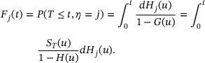
The CIF for type-j risk is  , and the cause-specific hazard function for type-j risk is
  , where
  . Let H represent the distribution function for X and further define the subdistribution functions
  . Therefore,
  is the distribution function for type-j uncensored failure time. The CIF for type-j risk can then be expressed as
We estimate the overall survival function  by the Kaplan–Meier estimator
  , distribution function H by
  . and subdistribution function
  by
by  , then the Aalen–Johansen estimator can be given by
By martingale theory and the functional delta method, asymptotic normality properties of a single CIF estimator have been studied by Bryant and Dignam (2004), Lin (1997), and Zhang and Fine (2008). Under Assumptions (A1) and (A2) in Web Appendix A,  converges weakly to a zero-mean Gaussian process
  , with more details described in Web Appendix B.
2.2 Joint Asymptotic Distribution of Two CIF Estimators
In this section, we study the joint asymptotic distribution of two CIF estimators,  and
and  ,
,  . The joint asymptotic distribution will be used as a tool to further study functional transformations of the CIFs, which will be seen in the later part of this paper. As the covariance formula of Andersen et al. (2012) did not provide explicit formulation, in Theorem 1 we derive the covariance matrix with an explicit formula.
(Andersen et al., 2012) Under Assumptions (A1)–(A3), which are described in Web Appendix A,  converges weakly to a bivariate Gaussian process
  . The derivation of the covariance matrix is provided in Web Appendix C.
Using Theorem 1, as linear transformations of two CIF estimators will automatically converge weakly to a Gaussian process, these properties will be used to find the asymptotic distributions of statistics constructed from multiple CIFs.
3 CIF Inference for Weighted Survival Times
In this section, we define the weighted survival time and present a nonparametric estimation of the CIF for weighted survival time. Let  , be a nonnegative valued random weight function for failure type-j. Note that the weight functions are allowed to vary for different competing events based on the study interests. In COVID-19 applications, this weight function may be chosen to reflect, for example, the WHO severity score measured longitudinally. Define the weighted survival time
Using  ,
,  is constructed to reflect the QOL in relation to survival time, which forms a contrast with the simple definition of T. The weighted survival time can be viewed as an extension of the Q-TWiST (Gelber et al., 1989), which is a special case of weighted survival time in noncompeting events setting.
Taking COVID-19 as an example, the ordinal WHO severity score is longitudinally collected from each hospitalized patient to measure the severity of illness over time. A larger value of the WHO score represents a worse disease outcome, and the score reflects disease severity and therefore QOL of patients. In our data application, the WHO scores can be used for constructing weight functions for different competing events. When using time to death as a clinical endpoint, because prolonging survival time with a lower WHO score is preferred, we may assign more weights to those time periods with lower WHO scores, so that the weighted time to death for those patients with better disease status or QOL is prolonged accordingly. In contrast, for time to hospital discharge (i.e., recovery), as a rapid recovery with mild symptoms represents a clinically meaningful benefit, we may assign less weight to those time periods with lower WHO scores to shorten the weighted time to recovery.
Under the competing risks setting, the censoring time C is assumed to be independent of  , and the marker process
  and survival time T are allowed to be correlated. Note that the weight function is allowed to depend on risk type and
  is unknown if the failure event is censored. The observed data can be expressed as
  , which are independent and identically distributed (i.i.d.) replicates of
  .
.
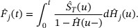
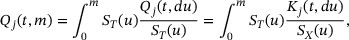
The CIF for type-j risk corresponding to the weighted survival time  is defined as
To estimate  , a natural estimator is the empirical distribution estimator
  provided that all the survival times of risk type j are uncensored. Clearly, this approach does not work in the presence of censoring. Below we propose a nonparametric estimation procedure that will resolve the problem.
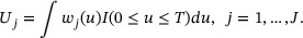
For a specific risk type  , we define
  . Then
  for any
  , where
  is the supremum of the support of T. Further define
  . Then, in the presence of censoring, under the assumption that C is independent of
  , one derives
where  . When the failure event is uncensored, both the risk type η and
  are observed and therefore
  can be estimated by its sample average, that is,
  . The function
  can also be estimated by sample average
  . By plugging into the Kaplan–Meier estimate
  and the empirical estimators
  ,
,  can be nonparametrically estimated by
for  .
.
For the special case that  , we may set
  and derive the estimator
  . For the general case that the condition
  may or may not be satisfied, we may select a time point
  and derive a restricted version of
  , named as
  , which is subject to the restriction that
  so that
  . For example, in a clinical trial setting, the survival time T of interest is typically restricted to a time interval
  , where τ is a prespecified ending time of the trial. The maximum follow-up time is designed to be longer than τ, which implies
  . In such cases, a nonparametric estimator of
  can then be obtained as
  .
.
Of note, if  , one still has
  by selecting
  . Also, knowledge of the weight functional values for censored observations (i.e., those observed times with
  ) is not needed in our estimation steps. In real data applications such as the COVID-19 example, the weight function depends on risk type and it is unknown if the failure event is censored.
Further define  ,
,  , and
, and  , in which
  is the cumulative hazard function of the censoring time C. Theorem 2 summarizes the asymptotic property of
  . The proof with details is included in Web Appendix D.
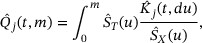
 and assume the validity of (A2)-(A3) and (B1) as described in Web Appendix A, the stochastic process
 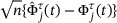 has an asymptotically i.i.d. representation
 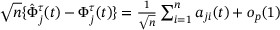 , where for
  ,
, 
As  ,
,  converges weakly to a zero-mean Gaussian process with covariance function
  . Moreover, as
  , for any
  , vector
  converges weakly to a zero-mean bivariate Gaussian process with covariance function
  .
.
The variance–covariance structure can be consistently estimated by  where
where  and
and  are obtained by replacing all the unknown parameters with their respective empirical estimates.
in which  is the inverse function of
  . Clearly, g is strictly increasing and the existence of
  is guaranteed. Thus, the weighted CIF
  can be viewed as the average of a rescaled CIF
  .
.
4 Analytical Methods for Clinical Trials with Bivariate Endpoints
RCTs with time-to-event outcomes are useful tools to identify effective interventions. Statistical analysis of restricted mean time (RMT) has been proposed and widely used to compare treatment and control groups using a single primary endpoint (Chen & Tsiatis, 2001; Karrison, 1987); Royston & Parmar, 2011, 2013; Zhang & Schaubel, 2011). By extending the analysis of RMT for a single endpoint, in this section we develop analytical tools using two competing endpoints in a clinical trial setting.
In a clinical trial focusing on COVID-19 infection or ICU treatment, with τ set as a prespecified ending time of the trial, discharge from the hospital, and death are the endpoints of hospitalization and can be treated as two competing events. By treating hospital discharge as the first endpoint with  and death as the second endpoint with
  , we define the time gained or lost due to the occurrence of a specific endpoint. In addition to COVID-19 treatment trials, a putative negative correlation between competing events also naturally arises in critical care (Resche-Rigon et al., 2005) and epileptic seizure (Williamson et al., 2007) clinical research, making the proposed research particularly desirable in multiple subdisciplines in medicine.
Specifically, for those who were discharged from the hospital, define their restricted gained time as  . Similarly, for those who died during their hospital stay, define their restricted lost time as
  . Then the restricted mean gained time (RMGT) and the restricted mean lost time (RMLT) can be, respectively, expressed as
In practice, the value of τ is determined based on research interest as well as the length of the study. Of note, with a focus on inference for a single event, RMT similar to  , has also been considered by Andersen (2013) and Uno et al. (2015) in competing risks models.
Figure 1 gives a graphic presentation of RMGT and RMLT, in which the x-axis is the time, the y-axis is the cumulative incidence, and τ is set to be 29 days. The lower curve in Figure 1 is the CIF of time to death; therefore, the RMLT is the area below that curve between 0 and day 29 (left-shaded area). Likewise, the upper curve in the figure is the summation of the CIF of time to death and the CIF of time to discharge; therefore, the RMGT is the area between two CIFs (right-shaded area). The remaining area on the left upper portion can be interpreted as the mean time spent in the hospital. The RMGT and RMLT are two key summary measures that directly correspond to recovery and death and characterize patients' disease development and eventual outcomes. The mean time of hospitalization is a direct measure of healthcare resource utilization, irrespective of treatment outcome.
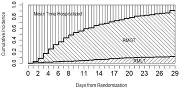
Explanation plot for RMGT and RMLT
The estimation of RMGT and RMLT can be easily constructed using the Aalen–Johansen's estimation approach (Aalen & Johansen, 1978). For  , a straightforward estimator is
  . Using the properties of CIF described in Section 2, the asymptotic variance of
  can be estimated by
in which  is the Kaplan—Meier estimator of the survival function for T,
  is the Aalen–Johansen estimator of the CIF for type-j risk,
  counts failure events prior to time t,
  counts type-j failure event priors to time t, and
  denotes the total number of subjects at risk at time t.
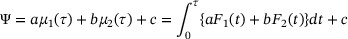
In COVID-19 clinical trials, an ideal intervention is expected to prolong lifetime with reduced mortality risk and shorten hospital stay with increased recovery probability, which correspond to smaller RMLT and larger RMGT. As discussed in Section 1, since there are multiple endpoints in the trial, considering just one endpoint may not give us a full picture of the disease progression. Therefore, to allow concrete interpretation and facilitate evidence synthesis, we propose to construct a treatment efficacy measure as a linear combination of RMGT and RMLT:
in which  are pre-specified weighting constants and these constants are subjectively defined, depending on investigators' interest.
If  then the efficacy measure Ψ corresponds to the “net” mean time (RMGT − RMLT), which directly reflects the effectiveness of the intervention.
Define a treatment efficacy measure using a linear combination of three areas (RMGT, RMLT, mean time in hospital) in Figure 1:  . Equivalently, a treatment efficacy measure is defined as
  , where
  . Note that
  (or
(or  ) means the trial effect does not take into account the mean time in the hospital.
By plugging in the Aalen–Johansen estimators for the CIFs  , we obtain a nonparametric estimator
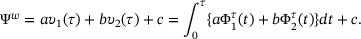
  . Similarly, using the weighted CIFs, we can also define the weighted restricted mean gained time (WRMGT) as
  and the weighted restricted mean lost time (WRMLT) as
  , in which
  and
and  are the weighted CIFs restricted to the time interval [0, τ] as defined in Section 3. An alternative efficacy measure can then be defined using two weighted CIFs:
By plugging into the estimators  proposed in Section 3,
  , we can derive a nonparametric estimator
  .
.
On the basis of properties of CIFs that we derived in Theorems 1 and 2, asymptotic normality properties of  and
and  can be established in Theorem 3 below. The proof can be found in Web Appendix D.
Under Assumptions (A1)–(A3) and (B1) in Web Appendix A, (i)  satisfies
  , and (ii)
  satisfies
  , in which σ2 and γ2 can be found in Web Appendix D.
Based on the large sample result described in Theorem 3, statistics for hypothesis testing can be developed to evaluate the intervention efficacy in clinical trials. We will use such test statistics in Section 6 for real data analysis.
5 Simulation Studies
We conduct Monte Carlo simulations to evaluate finite-sample properties of the proposed estimation and inference procedures for the joint distributions of CIFs (Scenario I) and weighted CIFs (Scenario II), respectively. Motivated by COVID-19 treatment trials, we focus on situations where there are two competing event types (e.g., recovery and death) and the two events have opposite clinical interpretations.
For Scenario I, we simulate bivariate latent failure times, each following a marginal exponential distribution, and use a Gaussian copula (Song, 2000) to induce a negative correlation between the two failure times. Their pairwise minimum leads to the uncensored competing risks data, with association summarized by Pearson's correlation coefficient. For Scenario II, to simulate competing risks data with longitudinal trajectories representing disease severity, we first consider trivariate latent failure times, corresponding to (1) death with monotonic deterioration, (2) monotonic recovery, and (3) U-shape recovery, respectively. The trivariate latent failure times are generated using marginal exponential distributions and Gaussian copula, similar to the generation process for bivariate failure times. For each simulated latent failure time t, the transitions between different severity are simulated randomly with a uniform distribution over (0, t). For both scenarios, different sample sizes (n = 100, 200, or 300) are considered, and independent censoring is introduced through a random variable with uniform distribution to achieve the desired proportion of censoring (20% or 50%). Additional details of the simulation setup, including the underlying distribution of simulated failure times, can be found in Web Appendix E.
Estimates of CIF and weighted CIF described in Sections 2 and 3 for both failure types at  , as well as their estimated variance/covariance, are summarized in Tables 1 and 2. Based on 1000 replications, the proposed estimators are seen to be approximately unbiased at all sample sizes evaluated. The empirical standard error (SE) and empirical mean of the standard error estimates (SEE) for a single CIF, as well as empirical covariance (cov) and empirical mean of the covariance estimates (covE) for their joint distribution, are consistently close to each other. As the sample size increases, the variance and covariance estimates also reduce accordingly at the expected convergence rate. Of note, when the sample size is small and the censoring rate is high (e.g., n = 100 with a 50% censoring rate), the variance estimation may not be satisfactory due to an inadequate number of uncensored events.
Simulation summary statistic Part I
| Asymptotic variance/covariance estimator for CIF estimators | ||||||||||
|---|---|---|---|---|---|---|---|---|---|---|
 |  |  | ||||||||
| Cen | n | t | Bias | SE | SEE | Bias | SE | SEE | cov | covE |
| 20% | 100 | 0.5 | 0.0002 | 0.0281 | 0.0284 | 0.0018 | 0.0402 | 0.0408 |  |  |
| 1 | 0.0010 | 0.0363 | 0.0366 | 0.0011 | 0.0485 | 0.0478 |  |  | ||
| 1.5 | −0.0017 | 0.0404 | 0.0405 | 0.0017 | 0.0493 | 0.0493 |  |  | ||
| 200 | 0.5 | 0.0003 | 0.0206 | 0.0203 | 0.0017 | 0.0293 | 0.0291 |  |  | |
| 1 | 0.0004 | 0.0260 | 0.0260 | 0.0018 | 0.0335 | 0.0340 |  |  | ||
| 1.5 | −0.0014 | 0.0293 | 0.0289 | 0.0024 | 0.0354 | 0.0351 |  |  | ||
| 300 | 0.5 | 0.0002 | 0.0171 | 0.0166 | 0.0016 | 0.0235 | 0.0238 |  |  | |
| 1 | 0.0006 | 0.0213 | 0.0213 | 0.0015 | 0.0270 | 0.0278 |  |  | ||
| 1.5 | −0.0007 | 0.0238 | 0.0237 | 0.0018 | 0.0283 | 0.0287 |  |  | ||
| 50% | 100 | 0.5 | −0.0004 | 0.0302 | 0.0302 | 0.0015 | 0.0431 | 0.0436 |  |  |
| 1 | −0.0006 | 0.0426 | 0.0422 | 0.0033 | 0.0563 | 0.0561 |  |  | ||
| 1.5 | −0.0033 | 0.0537 | 0.0516 | 0.0024 | 0.0669 | 0.0652 |  |  | ||
| 200 | 0.5 | −0.0001 | 0.0222 | 0.0216 | 0.0022 | 0.0313 | 0.0311 |  |  | |
| 1 | 0.0001 | 0.0307 | 0.0302 | 0.0029 | 0.0391 | 0.0399 |  |  | ||
| 1.5 | −0.0017 | 0.0387 | 0.0373 | 0.0042 | 0.0470 | 0.0469 |  |  | ||
| 300 | 0.5 | −0.0005 | 0.0179 | 0.0177 | −0.0001 | 0.0252 | 0.0254 |  |  | |
| 1 | −0.0001 | 0.0242 | 0.0248 | 0.0003 | 0.0319 | 0.0327 |  |  | ||
| 1.5 | −0.0014 | 0.0296 | 0.0308 | 0.0029 | 0.0384 | 0.0386 |  |  | ||
| Asymptotic variance/covariance estimator for CIF estimators | ||||||||||
|---|---|---|---|---|---|---|---|---|---|---|
| | | ||||||||
| Cen | n | t | Bias | SE | SEE | Bias | SE | SEE | cov | covE |
| 20% | 100 | 0.5 | 0.0002 | 0.0281 | 0.0284 | 0.0018 | 0.0402 | 0.0408 | | |
| 1 | 0.0010 | 0.0363 | 0.0366 | 0.0011 | 0.0485 | 0.0478 | | | ||
| 1.5 | −0.0017 | 0.0404 | 0.0405 | 0.0017 | 0.0493 | 0.0493 | | | ||
| 200 | 0.5 | 0.0003 | 0.0206 | 0.0203 | 0.0017 | 0.0293 | 0.0291 | | | |
| 1 | 0.0004 | 0.0260 | 0.0260 | 0.0018 | 0.0335 | 0.0340 | | | ||
| 1.5 | −0.0014 | 0.0293 | 0.0289 | 0.0024 | 0.0354 | 0.0351 | | | ||
| 300 | 0.5 | 0.0002 | 0.0171 | 0.0166 | 0.0016 | 0.0235 | 0.0238 | | | |
| 1 | 0.0006 | 0.0213 | 0.0213 | 0.0015 | 0.0270 | 0.0278 | | | ||
| 1.5 | −0.0007 | 0.0238 | 0.0237 | 0.0018 | 0.0283 | 0.0287 | | | ||
| 50% | 100 | 0.5 | −0.0004 | 0.0302 | 0.0302 | 0.0015 | 0.0431 | 0.0436 | | |
| 1 | −0.0006 | 0.0426 | 0.0422 | 0.0033 | 0.0563 | 0.0561 | | | ||
| 1.5 | −0.0033 | 0.0537 | 0.0516 | 0.0024 | 0.0669 | 0.0652 | | | ||
| 200 | 0.5 | −0.0001 | 0.0222 | 0.0216 | 0.0022 | 0.0313 | 0.0311 | | | |
| 1 | 0.0001 | 0.0307 | 0.0302 | 0.0029 | 0.0391 | 0.0399 | | | ||
| 1.5 | −0.0017 | 0.0387 | 0.0373 | 0.0042 | 0.0470 | 0.0469 | | | ||
| 300 | 0.5 | −0.0005 | 0.0179 | 0.0177 | −0.0001 | 0.0252 | 0.0254 | | | |
| 1 | −0.0001 | 0.0242 | 0.0248 | 0.0003 | 0.0319 | 0.0327 | | | ||
| 1.5 | −0.0014 | 0.0296 | 0.0308 | 0.0029 | 0.0384 | 0.0386 | | | ||
Note: Cen is the censoring rate; n is the sample size; t is the time when these standard errors/covariance are calculated; Bias is the empirical bias; SE is the empirical standard error; SEE is the empirical mean of the standard error estimates; cov is the empirical covariance; covE is the empirical mean of the covariance estimates.
Simulation summary statistic Part I
| Asymptotic variance/covariance estimator for CIF estimators | ||||||||||
|---|---|---|---|---|---|---|---|---|---|---|
| | | ||||||||
| Cen | n | t | Bias | SE | SEE | Bias | SE | SEE | cov | covE |
| 20% | 100 | 0.5 | 0.0002 | 0.0281 | 0.0284 | 0.0018 | 0.0402 | 0.0408 | | |
| 1 | 0.0010 | 0.0363 | 0.0366 | 0.0011 | 0.0485 | 0.0478 | | | ||
| 1.5 | −0.0017 | 0.0404 | 0.0405 | 0.0017 | 0.0493 | 0.0493 | | | ||
| 200 | 0.5 | 0.0003 | 0.0206 | 0.0203 | 0.0017 | 0.0293 | 0.0291 | | | |
| 1 | 0.0004 | 0.0260 | 0.0260 | 0.0018 | 0.0335 | 0.0340 | | | ||
| 1.5 | −0.0014 | 0.0293 | 0.0289 | 0.0024 | 0.0354 | 0.0351 | | | ||
| 300 | 0.5 | 0.0002 | 0.0171 | 0.0166 | 0.0016 | 0.0235 | 0.0238 | | | |
| 1 | 0.0006 | 0.0213 | 0.0213 | 0.0015 | 0.0270 | 0.0278 | | | ||
| 1.5 | −0.0007 | 0.0238 | 0.0237 | 0.0018 | 0.0283 | 0.0287 | | | ||
| 50% | 100 | 0.5 | −0.0004 | 0.0302 | 0.0302 | 0.0015 | 0.0431 | 0.0436 | | |
| 1 | −0.0006 | 0.0426 | 0.0422 | 0.0033 | 0.0563 | 0.0561 | | | ||
| 1.5 | −0.0033 | 0.0537 | 0.0516 | 0.0024 | 0.0669 | 0.0652 | | | ||
| 200 | 0.5 | −0.0001 | 0.0222 | 0.0216 | 0.0022 | 0.0313 | 0.0311 | | | |
| 1 | 0.0001 | 0.0307 | 0.0302 | 0.0029 | 0.0391 | 0.0399 | | | ||
| 1.5 | −0.0017 | 0.0387 | 0.0373 | 0.0042 | 0.0470 | 0.0469 | | | ||
| 300 | 0.5 | −0.0005 | 0.0179 | 0.0177 | −0.0001 | 0.0252 | 0.0254 | | | |
| 1 | −0.0001 | 0.0242 | 0.0248 | 0.0003 | 0.0319 | 0.0327 | | | ||
| 1.5 | −0.0014 | 0.0296 | 0.0308 | 0.0029 | 0.0384 | 0.0386 | | | ||
Note: Cen is the censoring rate; n is the sample size; t is the time when these standard errors/covariance are calculated; Bias is the empirical bias; SE is the empirical standard error; SEE is the empirical mean of the standard error estimates; cov is the empirical covariance; covE is the empirical mean of the covariance estimates.
Simulation summary statistic Part II
| Asymptotic variance/covariance estimator for weighted CIF estimators | |||||||||
|---|---|---|---|---|---|---|---|---|---|
 |  | ||||||||
| Cen | n | t | Bias | SE | SEE | Bias | SE | SEE | |
| 20% | 100 | 1 | −0.0018 | 0.0269 | 0.0269 | −0.0014 | 0.0333 | 0.0337 | |
| 2 | −0.0051 | 0.0354 | 0.0352 | −0.0008 | 0.0419 | 0.0428 | |||
| 3 | −0.0057 | 0.0389 | 0.0401 | −0.0034 | 0.0456 | 0.0469 | |||
| 4 | −0.0068 | 0.0411 | 0.0429 | −0.0059 | 0.0486 | 0.0489 | |||
| 200 | 1 | −0.0008 | 0.0187 | 0.0192 | −0.0012 | 0.0242 | 0.0239 | ||
| 2 | −0.0029 | 0.0252 | 0.0251 | −0.0008 | 0.0303 | 0.0302 | |||
| 3 | −0.0021 | 0.0279 | 0.0285 | −0.0022 | 0.0333 | 0.0332 | |||
| 4 | −0.0028 | 0.0292 | 0.0305 | −0.0041 | 0.0345 | 0.0346 | |||
| 300 | 1 | −0.0006 | 0.0156 | 0.0157 | −0.0015 | 0.0197 | 0.0195 | ||
| 2 | −0.0025 | 0.0209 | 0.0205 | −0.0012 | 0.0242 | 0.0247 | |||
| 3 | −0.0018 | 0.0233 | 0.0232 | −0.0013 | 0.0264 | 0.0271 | |||
| 4 | −0.0020 | 0.0246 | 0.0249 | −0.0029 | 0.0280 | 0.0282 | |||
| 50% | 100 | 1 | −0.0017 | 0.0277 | 0.0278 | −0.0016 | 0.0344 | 0.0348 | |
| 2 | −0.0056 | 0.0386 | 0.0385 | −0.0020 | 0.0459 | 0.0466 | |||
| 3 | −0.0057 | 0.0446 | 0.0469 | −0.0052 | 0.0534 | 0.0545 | |||
| 4 | −0.0091 | 0.0515 | 0.0549 | −0.0096 | 0.0611 | 0.0617 | |||
| 200 | 1 | −0.0008 | 0.0191 | 0.0199 | −0.0016 | 0.0251 | 0.0246 | ||
| 2 | −0.0032 | 0.0270 | 0.0274 | −0.0009 | 0.0329 | 0.0329 | |||
| 3 | −0.0035 | 0.0322 | 0.0332 | −0.0024 | 0.0388 | 0.0386 | |||
| 4 | −0.0051 | 0.0374 | 0.0391 | −0.0051 | 0.0440 | 0.0438 | |||
| 300 | 1 | −0.0005 | 0.0161 | 0.0163 | −0.0014 | 0.0203 | 0.0201 | ||
| 2 | −0.0025 | 0.0225 | 0.0224 | −0.0015 | 0.0262 | 0.0269 | |||
| 3 | −0.0019 | 0.0272 | 0.0273 | −0.0026 | 0.0303 | 0.0315 | |||
| 4 | −0.0026 | 0.0316 | 0.0320 | −0.0048 | 0.0356 | 0.0357 | |||
| Asymptotic variance/covariance estimator for weighted CIF estimators | |||||||||
|---|---|---|---|---|---|---|---|---|---|
| | ||||||||
| Cen | n | t | Bias | SE | SEE | Bias | SE | SEE | |
| 20% | 100 | 1 | −0.0018 | 0.0269 | 0.0269 | −0.0014 | 0.0333 | 0.0337 | |
| 2 | −0.0051 | 0.0354 | 0.0352 | −0.0008 | 0.0419 | 0.0428 | |||
| 3 | −0.0057 | 0.0389 | 0.0401 | −0.0034 | 0.0456 | 0.0469 | |||
| 4 | −0.0068 | 0.0411 | 0.0429 | −0.0059 | 0.0486 | 0.0489 | |||
| 200 | 1 | −0.0008 | 0.0187 | 0.0192 | −0.0012 | 0.0242 | 0.0239 | ||
| 2 | −0.0029 | 0.0252 | 0.0251 | −0.0008 | 0.0303 | 0.0302 | |||
| 3 | −0.0021 | 0.0279 | 0.0285 | −0.0022 | 0.0333 | 0.0332 | |||
| 4 | −0.0028 | 0.0292 | 0.0305 | −0.0041 | 0.0345 | 0.0346 | |||
| 300 | 1 | −0.0006 | 0.0156 | 0.0157 | −0.0015 | 0.0197 | 0.0195 | ||
| 2 | −0.0025 | 0.0209 | 0.0205 | −0.0012 | 0.0242 | 0.0247 | |||
| 3 | −0.0018 | 0.0233 | 0.0232 | −0.0013 | 0.0264 | 0.0271 | |||
| 4 | −0.0020 | 0.0246 | 0.0249 | −0.0029 | 0.0280 | 0.0282 | |||
| 50% | 100 | 1 | −0.0017 | 0.0277 | 0.0278 | −0.0016 | 0.0344 | 0.0348 | |
| 2 | −0.0056 | 0.0386 | 0.0385 | −0.0020 | 0.0459 | 0.0466 | |||
| 3 | −0.0057 | 0.0446 | 0.0469 | −0.0052 | 0.0534 | 0.0545 | |||
| 4 | −0.0091 | 0.0515 | 0.0549 | −0.0096 | 0.0611 | 0.0617 | |||
| 200 | 1 | −0.0008 | 0.0191 | 0.0199 | −0.0016 | 0.0251 | 0.0246 | ||
| 2 | −0.0032 | 0.0270 | 0.0274 | −0.0009 | 0.0329 | 0.0329 | |||
| 3 | −0.0035 | 0.0322 | 0.0332 | −0.0024 | 0.0388 | 0.0386 | |||
| 4 | −0.0051 | 0.0374 | 0.0391 | −0.0051 | 0.0440 | 0.0438 | |||
| 300 | 1 | −0.0005 | 0.0161 | 0.0163 | −0.0014 | 0.0203 | 0.0201 | ||
| 2 | −0.0025 | 0.0225 | 0.0224 | −0.0015 | 0.0262 | 0.0269 | |||
| 3 | −0.0019 | 0.0272 | 0.0273 | −0.0026 | 0.0303 | 0.0315 | |||
| 4 | −0.0026 | 0.0316 | 0.0320 | −0.0048 | 0.0356 | 0.0357 | |||
Note: Cen is the censoring rate; n is the sample size; t is the time when these standard errors/covariance are calculated; Bias is the empirical bias; SE is the empirical standard error; SEE is the empirical mean of the standard error estimates. The weighting procedure can be found in Web Appendix E.
Simulation summary statistic Part II
| Asymptotic variance/covariance estimator for weighted CIF estimators | |||||||||
|---|---|---|---|---|---|---|---|---|---|
| | ||||||||
| Cen | n | t | Bias | SE | SEE | Bias | SE | SEE | |
| 20% | 100 | 1 | −0.0018 | 0.0269 | 0.0269 | −0.0014 | 0.0333 | 0.0337 | |
| 2 | −0.0051 | 0.0354 | 0.0352 | −0.0008 | 0.0419 | 0.0428 | |||
| 3 | −0.0057 | 0.0389 | 0.0401 | −0.0034 | 0.0456 | 0.0469 | |||
| 4 | −0.0068 | 0.0411 | 0.0429 | −0.0059 | 0.0486 | 0.0489 | |||
| 200 | 1 | −0.0008 | 0.0187 | 0.0192 | −0.0012 | 0.0242 | 0.0239 | ||
| 2 | −0.0029 | 0.0252 | 0.0251 | −0.0008 | 0.0303 | 0.0302 | |||
| 3 | −0.0021 | 0.0279 | 0.0285 | −0.0022 | 0.0333 | 0.0332 | |||
| 4 | −0.0028 | 0.0292 | 0.0305 | −0.0041 | 0.0345 | 0.0346 | |||
| 300 | 1 | −0.0006 | 0.0156 | 0.0157 | −0.0015 | 0.0197 | 0.0195 | ||
| 2 | −0.0025 | 0.0209 | 0.0205 | −0.0012 | 0.0242 | 0.0247 | |||
| 3 | −0.0018 | 0.0233 | 0.0232 | −0.0013 | 0.0264 | 0.0271 | |||
| 4 | −0.0020 | 0.0246 | 0.0249 | −0.0029 | 0.0280 | 0.0282 | |||
| 50% | 100 | 1 | −0.0017 | 0.0277 | 0.0278 | −0.0016 | 0.0344 | 0.0348 | |
| 2 | −0.0056 | 0.0386 | 0.0385 | −0.0020 | 0.0459 | 0.0466 | |||
| 3 | −0.0057 | 0.0446 | 0.0469 | −0.0052 | 0.0534 | 0.0545 | |||
| 4 | −0.0091 | 0.0515 | 0.0549 | −0.0096 | 0.0611 | 0.0617 | |||
| 200 | 1 | −0.0008 | 0.0191 | 0.0199 | −0.0016 | 0.0251 | 0.0246 | ||
| 2 | −0.0032 | 0.0270 | 0.0274 | −0.0009 | 0.0329 | 0.0329 | |||
| 3 | −0.0035 | 0.0322 | 0.0332 | −0.0024 | 0.0388 | 0.0386 | |||
| 4 | −0.0051 | 0.0374 | 0.0391 | −0.0051 | 0.0440 | 0.0438 | |||
| 300 | 1 | −0.0005 | 0.0161 | 0.0163 | −0.0014 | 0.0203 | 0.0201 | ||
| 2 | −0.0025 | 0.0225 | 0.0224 | −0.0015 | 0.0262 | 0.0269 | |||
| 3 | −0.0019 | 0.0272 | 0.0273 | −0.0026 | 0.0303 | 0.0315 | |||
| 4 | −0.0026 | 0.0316 | 0.0320 | −0.0048 | 0.0356 | 0.0357 | |||
Note: Cen is the censoring rate; n is the sample size; t is the time when these standard errors/covariance are calculated; Bias is the empirical bias; SE is the empirical standard error; SEE is the empirical mean of the standard error estimates. The weighting procedure can be found in Web Appendix E.
We also evaluate finite sample properties of restricted-mean-based estimators Ψ, as described in Section 4. Results based on simulated data from Scenario I are summarized in Table 3. Using the COVID-19 trial as an example, the RMGT, RMLT, and their difference are expressed in terms of their linear transformations and evaluated at different τ values (τ = 0.5, 1, 1.5). Table 3 confirms that the proposed estimators and the associated variance estimators all perform well as expected.
Simulation summary statistic Part III
| Asymptotic behavior for the restricted mean time | |||||||||||
|---|---|---|---|---|---|---|---|---|---|---|---|
 |  |  | |||||||||
| (a = c = 0, b = 1) | (a = c = 0, b = 0) | (a = b = 1, c = −1) | |||||||||
| Cen | n | τ | Bias | SE | SEE | Bias | SE | SEE | Bias | SE | SEE |
| 20% | 100 | 0.5 | −0.0002 | 0.0086 | 0.0083 | 0.0007 | 0.0126 | 0.0126 | −0.0009 | 0.0159 | 0.0160 |
| 1 | −0.0001 | 0.0226 | 0.0226 | 0.0015 | 0.0314 | 0.0317 | −0.0015 | 0.0425 | 0.0434 | ||
| 1.5 | −0.0004 | 0.0392 | 0.0396 | 0.0028 | 0.0523 | 0.0521 | −0.0032 | 0.0749 | 0.0764 | ||
| 200 | 0.5 | −0.0001 | 0.0061 | 0.0060 | 0.0005 | 0.0090 | 0.0090 | −0.0005 | 0.0116 | 0.0114 | |
| 1 | −0.0001 | 0.0163 | 0.0162 | 0.0015 | 0.0224 | 0.0225 | −0.0015 | 0.0309 | 0.0309 | ||
| 1.5 | −0.0004 | 0.0284 | 0.0283 | 0.0033 | 0.0370 | 0.0370 | −0.0037 | 0.0543 | 0.0543 | ||
| 300 | 0.5 | −0.0001 | 0.0050 | 0.0049 | 0.0005 | 0.0072 | 0.0073 | −0.0005 | 0.0093 | 0.0094 | |
| 1 | 0.0001 | 0.0134 | 0.0133 | 0.0015 | 0.0180 | 0.0184 | −0.0014 | 0.0249 | 0.0253 | ||
| 1.5 | −0.0002 | 0.0233 | 0.0232 | 0.0030 | 0.0298 | 0.0303 | −0.0032 | 0.0439 | 0.0445 | ||
| 50% | 100 | 0.5 | −0.0002 | 0.0090 | 0.0086 | 0.0006 | 0.0131 | 0.0130 | −0.0008 | 0.0165 | 0.0165 |
| 1 | −0.0002 | 0.0245 | 0.0242 | 0.0011 | 0.0336 | 0.0338 | −0.0013 | 0.0458 | 0.0462 | ||
| 1.5 | −0.0012 | 0.0443 | 0.0439 | 0.0023 | 0.0579 | 0.0579 | −0.0035 | 0.0842 | 0.0843 | ||
| 200 | 0.5 | −0.0001 | 0.0063 | 0.0062 | 0.0006 | 0.0093 | 0.0092 | −0.0006 | 0.0120 | 0.0118 | |
| 1 | 0.0001 | 0.0177 | 0.0173 | 0.0015 | 0.0239 | 0.0240 | −0.0014 | 0.0333 | 0.0330 | ||
| 1.5 | −0.0003 | 0.0323 | 0.0314 | 0.0034 | 0.0410 | 0.0412 | −0.0037 | 0.0608 | 0.0602 | ||
| 300 | 0.5 | −0.0001 | 0.0005 | 0.0005 | 0.0005 | 0.0075 | 0.0075 | −0.0006 | 0.0096 | 0.0096 | |
| 1 | −0.0001 | 0.0140 | 0.0142 | 0.0015 | 0.0193 | 0.0197 | −0.0016 | 0.0263 | 0.0269 | ||
| 1.5 | −0.0004 | 0.0249 | 0.0257 | 0.0029 | 0.0333 | 0.0338 | −0.0033 | 0.0479 | 0.0492 | ||
| Asymptotic behavior for the restricted mean time | |||||||||||
|---|---|---|---|---|---|---|---|---|---|---|---|
| | | |||||||||
| (a = c = 0, b = 1) | (a = c = 0, b = 0) | (a = b = 1, c = −1) | |||||||||
| Cen | n | τ | Bias | SE | SEE | Bias | SE | SEE | Bias | SE | SEE |
| 20% | 100 | 0.5 | −0.0002 | 0.0086 | 0.0083 | 0.0007 | 0.0126 | 0.0126 | −0.0009 | 0.0159 | 0.0160 |
| 1 | −0.0001 | 0.0226 | 0.0226 | 0.0015 | 0.0314 | 0.0317 | −0.0015 | 0.0425 | 0.0434 | ||
| 1.5 | −0.0004 | 0.0392 | 0.0396 | 0.0028 | 0.0523 | 0.0521 | −0.0032 | 0.0749 | 0.0764 | ||
| 200 | 0.5 | −0.0001 | 0.0061 | 0.0060 | 0.0005 | 0.0090 | 0.0090 | −0.0005 | 0.0116 | 0.0114 | |
| 1 | −0.0001 | 0.0163 | 0.0162 | 0.0015 | 0.0224 | 0.0225 | −0.0015 | 0.0309 | 0.0309 | ||
| 1.5 | −0.0004 | 0.0284 | 0.0283 | 0.0033 | 0.0370 | 0.0370 | −0.0037 | 0.0543 | 0.0543 | ||
| 300 | 0.5 | −0.0001 | 0.0050 | 0.0049 | 0.0005 | 0.0072 | 0.0073 | −0.0005 | 0.0093 | 0.0094 | |
| 1 | 0.0001 | 0.0134 | 0.0133 | 0.0015 | 0.0180 | 0.0184 | −0.0014 | 0.0249 | 0.0253 | ||
| 1.5 | −0.0002 | 0.0233 | 0.0232 | 0.0030 | 0.0298 | 0.0303 | −0.0032 | 0.0439 | 0.0445 | ||
| 50% | 100 | 0.5 | −0.0002 | 0.0090 | 0.0086 | 0.0006 | 0.0131 | 0.0130 | −0.0008 | 0.0165 | 0.0165 |
| 1 | −0.0002 | 0.0245 | 0.0242 | 0.0011 | 0.0336 | 0.0338 | −0.0013 | 0.0458 | 0.0462 | ||
| 1.5 | −0.0012 | 0.0443 | 0.0439 | 0.0023 | 0.0579 | 0.0579 | −0.0035 | 0.0842 | 0.0843 | ||
| 200 | 0.5 | −0.0001 | 0.0063 | 0.0062 | 0.0006 | 0.0093 | 0.0092 | −0.0006 | 0.0120 | 0.0118 | |
| 1 | 0.0001 | 0.0177 | 0.0173 | 0.0015 | 0.0239 | 0.0240 | −0.0014 | 0.0333 | 0.0330 | ||
| 1.5 | −0.0003 | 0.0323 | 0.0314 | 0.0034 | 0.0410 | 0.0412 | −0.0037 | 0.0608 | 0.0602 | ||
| 300 | 0.5 | −0.0001 | 0.0005 | 0.0005 | 0.0005 | 0.0075 | 0.0075 | −0.0006 | 0.0096 | 0.0096 | |
| 1 | −0.0001 | 0.0140 | 0.0142 | 0.0015 | 0.0193 | 0.0197 | −0.0016 | 0.0263 | 0.0269 | ||
| 1.5 | −0.0004 | 0.0249 | 0.0257 | 0.0029 | 0.0333 | 0.0338 | −0.0033 | 0.0479 | 0.0492 | ||
Note: Cen is the censoring rate; n is the sample size; τ is the prespecified constant in the integral; Bias is the empirical bias; SE is the empirical standard error; SEE is the empirical mean of the standard error estimates.
Simulation summary statistic Part III
| Asymptotic behavior for the restricted mean time | |||||||||||
|---|---|---|---|---|---|---|---|---|---|---|---|
| | | |||||||||
| (a = c = 0, b = 1) | (a = c = 0, b = 0) | (a = b = 1, c = −1) | |||||||||
| Cen | n | τ | Bias | SE | SEE | Bias | SE | SEE | Bias | SE | SEE |
| 20% | 100 | 0.5 | −0.0002 | 0.0086 | 0.0083 | 0.0007 | 0.0126 | 0.0126 | −0.0009 | 0.0159 | 0.0160 |
| 1 | −0.0001 | 0.0226 | 0.0226 | 0.0015 | 0.0314 | 0.0317 | −0.0015 | 0.0425 | 0.0434 | ||
| 1.5 | −0.0004 | 0.0392 | 0.0396 | 0.0028 | 0.0523 | 0.0521 | −0.0032 | 0.0749 | 0.0764 | ||
| 200 | 0.5 | −0.0001 | 0.0061 | 0.0060 | 0.0005 | 0.0090 | 0.0090 | −0.0005 | 0.0116 | 0.0114 | |
| 1 | −0.0001 | 0.0163 | 0.0162 | 0.0015 | 0.0224 | 0.0225 | −0.0015 | 0.0309 | 0.0309 | ||
| 1.5 | −0.0004 | 0.0284 | 0.0283 | 0.0033 | 0.0370 | 0.0370 | −0.0037 | 0.0543 | 0.0543 | ||
| 300 | 0.5 | −0.0001 | 0.0050 | 0.0049 | 0.0005 | 0.0072 | 0.0073 | −0.0005 | 0.0093 | 0.0094 | |
| 1 | 0.0001 | 0.0134 | 0.0133 | 0.0015 | 0.0180 | 0.0184 | −0.0014 | 0.0249 | 0.0253 | ||
| 1.5 | −0.0002 | 0.0233 | 0.0232 | 0.0030 | 0.0298 | 0.0303 | −0.0032 | 0.0439 | 0.0445 | ||
| 50% | 100 | 0.5 | −0.0002 | 0.0090 | 0.0086 | 0.0006 | 0.0131 | 0.0130 | −0.0008 | 0.0165 | 0.0165 |
| 1 | −0.0002 | 0.0245 | 0.0242 | 0.0011 | 0.0336 | 0.0338 | −0.0013 | 0.0458 | 0.0462 | ||
| 1.5 | −0.0012 | 0.0443 | 0.0439 | 0.0023 | 0.0579 | 0.0579 | −0.0035 | 0.0842 | 0.0843 | ||
| 200 | 0.5 | −0.0001 | 0.0063 | 0.0062 | 0.0006 | 0.0093 | 0.0092 | −0.0006 | 0.0120 | 0.0118 | |
| 1 | 0.0001 | 0.0177 | 0.0173 | 0.0015 | 0.0239 | 0.0240 | −0.0014 | 0.0333 | 0.0330 | ||
| 1.5 | −0.0003 | 0.0323 | 0.0314 | 0.0034 | 0.0410 | 0.0412 | −0.0037 | 0.0608 | 0.0602 | ||
| 300 | 0.5 | −0.0001 | 0.0005 | 0.0005 | 0.0005 | 0.0075 | 0.0075 | −0.0006 | 0.0096 | 0.0096 | |
| 1 | −0.0001 | 0.0140 | 0.0142 | 0.0015 | 0.0193 | 0.0197 | −0.0016 | 0.0263 | 0.0269 | ||
| 1.5 | −0.0004 | 0.0249 | 0.0257 | 0.0029 | 0.0333 | 0.0338 | −0.0033 | 0.0479 | 0.0492 | ||
Note: Cen is the censoring rate; n is the sample size; τ is the prespecified constant in the integral; Bias is the empirical bias; SE is the empirical standard error; SEE is the empirical mean of the standard error estimates.
6 Data Analysis: ACTT-1 Treatment Trial
To illustrate the analysis strategy proposed in Section 4, we conduct analysis using data from the Adaptive COVID-19 Treatment Trial (ACTT-1). This was a double-blind, randomized, placebo-controlled phase III trial to evaluate intravenous remdesivir in adults who were hospitalized with COVID-19 and had evidence of lower respiratory tract infection. The details of study design, conduct, and preplanned analysis results, including those based on standard survival analysis methods, can be found in Beigel et al. (2020). The study found that remdesivir significantly accelerated the time to recovery, while the mortality rate was significantly reduced only for a time interval of 1–15 days but not for 1–29 days. For illustrative purposes, out of the 1062 randomized patients, we excluded 18 patients who withdrew consent early with no follow-up or longitudinal information. There were four patients who died soon after hospital discharges. These four patients were considered “discharge-to-die” cases, and we treat them as death events. Our analysis thus consists of 529 on the remdesivir arm and 515 on the placebo arm.
Using standard CIFs and the asymptotic variance estimators described in Section 4, we report the analysis result of RMGT and RMLT, evaluated up to τ = 15 and 29 Days, for both arms, respectively. The differences in RMGT and RMLT between arms are used for treatment comparisons, with the Z-test for hypothesis testing. As shown in Table 4, the restricted mean gain time due to recovery is significantly longer in the remdesivir arm (1.379 days longer [95% CI: 0.812,1.946] over 15 days, and 2.786 days longer [95% CI: 1.597-3.976] over 29 days, p <0.001 for both), all indicating that remdesivir indeed accelerated recovery. Meanwhile, the RMLT attributed to morality is significantly reduced by 0.426 days (95% CI: 0.128-0.725, p = 0.005) over 15 days and 0.949 days (95% CI: 0.192-1.705, p = 0.014) over 29 days. Moreover, the “net” lifetime gained, using RMGT subtracting RMLT, is significantly longer in the remdesivir arm when evaluated over the first 15 days (4.724 days vs. 2.919 days, p <0.001) or 29 days (13.163 days vs. 9.428 days, p <0.001). Such a benefit-risk evaluation further confirms the benefit of remdesivir.
Restricted mean time analysis in ACTT-1 study
| Part I: Analysis results using standard CIF | ||
| Treatment group (days) | Control group (days) | |
| Day 15 | ||
| Restricted mean lost time (RMLT) | 0.520 (0.341–0.699) | 0.946 (0.707–1.186) |
| Difference (95% CI) | 0.426 (0.128-0.725), p-value=0.005 | |
| Restricted mean gain time (RMGT) | 5.244 (4.833–5.654) | 3.865 (3.474–4.256) |
| Difference (95% CI) | 1.379 (0.812-1.946), p-value<0.0001 | |
| “Net” mean time (RMGT-RMLT) | 4.724 (4.241–5.207) | 2.919 (2.413–3.425) |
| Difference (95% CI) | 1.805 (1.106-2.504), p-value<0.0001 | |
| Day 29 | ||
| Restricted mean lost time (RMLT) | 1.902 (1.436–2.369) | 2.851 (2.256–3.446) |
| Difference (95% CI) | 0.949 (0.192-1.705), p-value=0.014 | |
| Restricted mean gain time (RMGT) | 15.065 (14.231–15.899) | 12.279 (11.430–13.127) |
| Difference (95% CI) | 2.786 (1.597-3.976), p-value<0.0001 | |
| “Net” mean time (RMGT-RMLT) | 13.163 (12.035–14.291) | 9.428 (8.193–10.662) |
| Difference (95% CI) | 3.735 (2.063-5.407), p-value<0.0001 | |
| Part II: Analysis results using weighted CIF | ||
| Treatment group (days) | Control group (days) | |
| Day 15 | ||
| Weighted restricted mean lost time (WRMLT) | 0.722 (0.481–0.963) | 1.119 (0.814–1.424) |
| Difference (95% CI) | 0.397 (0.008-0.786), p-value=0.046 | |
| Weighted restricted mean gain time (WRMGT) | 4.856 (4.383–5.329) | 3.605 (3.154–4.056) |
| Difference (95% CI) | 1.251 (0.598-1.905), p-value=0.0002 | |
| Day 29 | ||
| Weighted restricted mean lost time (WRMLT) | 2.134 (1.423–2.846) | 3.044 (2.296–3.792) |
| Difference (95% CI) | 0.910 (-0.123-1.942), p-value=0.084 | |
| Weighted restricted mean gain time (WRMGT) | 13.128 (12.153–14.103) | 10.328 (9.348–11.307) |
| Difference (95% CI) | 2.800 (1.419-4.182), p-value<0.0001 | |
By incorporating the longitudinally assessed WHO severity information, the weighted CIF analysis on the scale of RMT provides stakeholders a tailored analysis of particular interest. For example, by assigning weight utility of (2, 1.5, 1, 0.5) for WHO scores (4, 5, 6, 7), the WRMLT reflects the significantly “discounted” life quality when ventilation is used. On the other hand, a weighte utility of (0.5, 1, 1.5, 2) for WHO scores (4, 5, 6, 7) in the WRMGT analysis produces a shorter weighted time-to-discharge for patients with good QOL. By incorporating such weights into the analysis, the weighted RMGT is significantly longer in the remdesivir arm (1.251 days longer [95% CI: 0.598-1.905] over 15 days, and 2.800 days longer [95% CI: 1.419-4.182] over 29 days, p<0.001 for both), indicating remdesivir improved recovery from the QOL perspective. In the meantime, a reduction in the weighted RMLT attributed to morality is 0.397 days (95% CI: 0.008-0.786, p = 0.046) over 15 days but the reduction does not show a significant difference over 29 days when taking into account the QOL (0.910 days, [95% CI: -0.123-1.942], p = 0.084).
7 Discussion
In this paper, we develop joint inference for multiple CIFs for competing risks models. An analytical plan based on RMT for comparative clinical trials is developed based on competing risks data. Using the COVID-19 trial data we demonstrate that the proposed methods are especially useful when two competing events both have meaningful but opposite clinical interpretations. The proposed methods can also be adapted to study chronic diseases when composite endpoints are used regularly to evaluate the association between treatment and multiple components of the composite endpoint (e.g., death and recurrence of cancer). Furthermore, numerous test statistics based on multiple competing events have been developed and we expect the analysis based on these test statistics will be published and used with wider applications in the future.
As we argue in earlier sections, the joint inference tools for multiple CIFs together with methods based on the RMT are expected to provide intriguing insights to physicians, patients, and health administrators to facilitate their decision making. From a study design perspective, a joint inference framework presumably provides an opportunity to reduce sample sizes and increase power by detecting a difference in CIF of any competing event, which is a topic of future research. In addition, as it is well known that covariate adjustment would typically increase estimation precision in linear models, it would be of interest to investigate if adjusting baseline prognostic factors may increase the estimation precision of RMT in competing risks models.
Data Availability Statement
The data that support the findings in this paper are available from the National Institutes of Health. Restrictions apply to the availability of these data, which were used under license in this paper. Data are available from the authors with the permission of the National Institutes of Health.
Acknowledgments
Jiyang Wen is supported by NIH Grant U01 AG051412. Chen Hu is supported in part by NIH Grant U10-CA180822. Mei-Cheng Wang is supported in part by NIH Grant U19 AG033655.
References
