


Abstract
Statistical analysis of longitudinal data often involves modeling treatment effects on clinically relevant longitudinal biomarkers since an initial event (the time origin). In some studies including preventive HIV vaccine efficacy trials, some participants have biomarkers measured starting at the time origin, whereas others have biomarkers measured starting later with the time origin unknown. The semiparametric additive time-varying coefficient model is investigated where the effects of some covariates vary nonparametrically with time while the effects of others remain constant. Weighted profile least squares estimators coupled with kernel smoothing are developed. The method uses the expectation maximization approach to deal with the censored time origin. The Kaplan–Meier estimator and other failure time regression models such as the Cox model can be utilized to estimate the distribution and the conditional distribution of left censored event time related to the censored time origin. Asymptotic properties of the parametric and nonparametric estimators and consistent asymptotic variance estimators are derived. A two-stage estimation procedure for choosing weight is proposed to improve estimation efficiency. Numerical simulations are conducted to examine finite sample properties of the proposed estimators. The simulation results show that the theory and methods work well. The efficiency gain of the two-stage estimation procedure depends on the distribution of the longitudinal error processes. The method is applied to analyze data from the Merck 023/HVTN 502 Step HIV vaccine study.
1 Introduction
In preventive HIV vaccine efficacy trials, thousands of HIV uninfected volunteers are randomized to receive vaccine or placebo, and are monitored for HIV infection. Participants diagnosed with HIV infection have various endpoints measured longitudinally starting at the date of diagnosis; these endpoints include viral loads and CD4 cell counts as markers of HIV disease progression and secondary transmission. An objective of such trials is to assess the vaccine effect on the biomarkers, and all previous analyses assessed the biomarkers based on the time from HIV diagnosis (Fitzgerald et al., 2011; Rerks-Ngarm et al., 2013; Janes et al., 2015). However, it is more biologically meaningful to assess whether vaccination modifies the biomarkers over time since actual HIV acquisition. This assessment is challenging because exact times of HIV acquisition are generally unobtainable; rather data are available only on bounds  and
and  between which the true time origin must lie
  , where, as shown in Figure 1, for example,
  is the date of the last antibody (Ab)-based HIV negative diagnostic test result and
  is the date of the first antibody (Ab)-based HIV positive test result. Given details of the HIV testing algorithm described in the application, some participants have
  , at least approximately, such that
  is considered to be directly observed, whereas other participants have
  and
and  is unknown. This set-up occurs in other multi-stage longitudinal studies, as depicted in Figure 1.
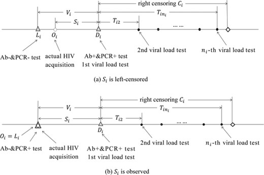
Censored time origin  in the study of a longitudinal response. Based on the HIV testing algorithm, each infected participant was classified into one of two groups, defined by whether the earliest HIV positive sample was (Ab+, PCR+) or (Ab-, PCR+). (a) For participants with the earliest HIV positive sample (Ab+, PCR+),
  is left censored by
  ; (b) For participants with the earliest HIV positive sample (Ab-, PCR+),
  and
and  is observed
In Figure 1, for each participant  ,
,  is the gap time between the true time origin
  and the time
  when longitudinal markers begin to be measured. The time lapse from
  and
and  is
is  . For participant i, the longitudinal markers are measured at times
  , where
  is the time between
  and the jth marker measurement, for
  . In the HIV vaccine study, most participants have first measurement time
  at
at  ; some participants have
  and others have
  . Formally, we write
  and
and  such that
  is left censored by
  with censoring indicator
  ;
;  is observed if
  and
and  if
if  . The time from
  to the jth sampling time is
  . The time origin is considered censored because
  is left censored.
Semiparametric regression models for longitudinal data have been intensively studied; see Lin and Ying (2001), Hu et al. (2004), Qu and Li (2006), Fan et al. (2007) and Sun et al. (2013), among others. However, to the best of our knowledge, none of these methods address the problem in which the time origin may be censored. In this paper, we study the semiparametric additive model with time-varying effects for longitudinal data with censored time origin. Weighted profile least squares estimators are developed for the unknown parameters as well as for the nonparametric coefficient functions. The expectation maximization approach is utilized to deal with the censored time origin. The proposed method does not assume any specific model for the sampling times, and thus avoids misspecification of the sampling models. The method is applied to investigate the effect of an HIV vaccine on viral load over time since actual HIV acquisition in the Merck 023/HVTN 502 Step study. Asymptotic properties of the parametric and nonparametric estimators and consistent asymptotic variance estimators are derived. Our numerical study shows that the proposed methods work well with satisfying finite sample properties.
The rest of the paper is organized as follows. Section 2 introduces the semiparametric additive model and develops the estimation method. Preliminaries on the data structure and model assumptions are given in Section 2.1. The weighted profile least squares estimators coupled with the kernel smoothing and EM algorithm are developed in Section 2.2. Computational issues about estimation at the boundaries and the weight selection are discussed in Section 2.3. In Section 3, we establish asymptotic properties of the nonparametric and parametric estimators, and in Section 4 study their finite sample performances in simulations. The proposed method is applied to Step trial in Section 5. Concluding remarks are given in Section 6. The proofs of the asymptotic results, additional simulations and data analysis, and the discussions on bandwidth choice are placed in Web Appendices available in the Supporting Information of this article.
2 Profile Weighted Least Squares Estimation through EM Algorithm
2.1 Preliminaries
Suppose that there is a random sample of n participants. For participant i, let  be the response process and let
  and
and  be possibly time-dependent covariates of dimensions
  and
and  , respectively, where
  is the time since the actual time origin, and τ is the study duration. We consider the following semiparametric additive time-varying coefficients model

where  is an unspecified
  vector of smooth regression functions, γ is a
  dimensional vector of parameters, and
  is a mean-zero process. The notation
  represents transpose of a vector or matrix x. Specify the first component of
  as 1 gives a model with a nonparametric baseline response process. The effect of
  is time-varying modeled nonparametrically while the effect of
  is time-independent modeled parametrically.
The observations of  are taken at time points
  , where
  is the total number of observations from the ith subject. The
  can be written as the sum of two parts
  as shown in Figure 1, where
  is the time from the actual time origin
  participant to left censoring by
  , and
, and  is the time from the right edge
  of the interval for
  to the jth visit for the ith subject, where visit 1 is at
  . Let
. Let  be the end of follow-up time or censoring time for the ith participant since
  . The censoring time
  is allowed to depend on the covariates
  and
and  . The responses for the ith participant can only be observed at the time points before
  since the actual time origin.
The sampling times  may vary among participants. The number of observations taken from the ith participant by time t is
  , where
  is the indicator function. Let
  be the conditional mean rate of the sampling times for participant i at time t defined by
  ,
,  . The mean rate function is assumed to only depend on
  , which is the part of the covariates
  that affects the potential sampling times. We denote
  , where
  is an unspecified nonnegative smooth function.
Let  ,
,  ,
,  ,
,  ,
,  ,
,  ,
,  , where
  is a collection of possible auxiliary variables that are not of interest in the modeling of
  but may be useful in predicting the distribution of
  . For the censored time origin, left-censored data
  and
and  are observed. The observed data for participant i can be expressed as
  . The observation is
  if
if  and
and  if
if  , where
  . Although exact times
  may be unobtainable, the values
  ,
,  and
and  at
at  are known. Assume that
  are independent identically distributed (iid). The observed data are denoted by
  .
.
We assume that  and
and  are independent conditional on
  , and that the censoring time
  is noninformative in that
 ,
,  and
and  ,
,  . Let
. Let  . Assume
  ,
, 
 ,
,  ,
,  ,
,  ,
,  . Assume also that
  and
and  are independent conditional on
  ,
,  , and
, and  . This assumption implies that, conditional on covariate processes, sampling times are noninformative for the longitudinal response.
2.2 Estimation Procedures
When all  's are observed, estimation procedure such as in Sun and Wu (2005) and Sun et al. (2013) can be used to analyze model (1). If the unobserved or censored
  's are treated as missing, then
  is not missing at random. The inverse probability weighting of complete-cases method and the augmented inverse probability weighted complete-case method of Robins et al. (1994), which have been successfully adapted in Sun and Gilbert (2012), Sun et al. (2017), Yang et al. (2017) and by many other authors, will not work in this situation. We propose an estimation procedure based on the missing-data principle using the EM-algorithm.
The conditional distribution  of
of  equals
 for
for  and 1 for
  . Let
. Let  be the estimated conditional distribution of
  . Let
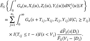
. Let  . The estimation of model (1) can be based on minimizing the following objective function:
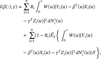
where  is a nonnegative weight function, and
  is the estimate of the conditional expectation
  , which can be obtained through estimation of
  as we show below.
For ease of presentation, we adopt the notation 

 for
for 
 ,
,  ,
,  , where
  is a smooth function of
  . The above objective function can be written as
Note that  ,
,  and
and  are observed. The conditional expectation
  for participant i with
  equals
where the last equality holds because  for
for  . Since
  , estimating
  by
by  for
for  , we have
The basic idea of estimating the conditional distribution  is to transform the data set from left censored to right censored. Assume that
  is bounded by a predetermined constant L. This is reasonable since for the application concerned here
  is less than the time interval between two consecutive testing times that is usually between 3 and 6 months. The distribution of
  based on the left censored data can be estimated by the methods developed for right censored data through the transformation
  . The Kaplan–Meier estimator can be used to estimate distribution of
  when
when  is independent of
  . Otherwise, a failure time regression model such as the Cox model can be used to estimate the conditional distribution
  .
.
Next, we present an estimation procedure that estimates the nonparametric component  with the kernel smoothing and the parametric component γ with the profile weighted least squares method. Let
  be a symmetric kernel function with compact support. For fixed γ and at time t, we estimate
  by minimizing the following objective function with respect to β:
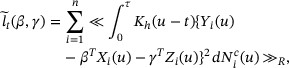
where  and h is the bandwidth depending on n.
Taking the derivative of  with respect to β for a fixed γ yields
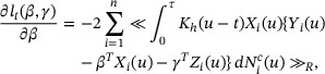
which leads to the following estimating function
Let 


 , and define
  and
and  similarly by replacing
  with
with  , and
, and  with
with  , respectively. Solving
  for fixed γ and t yields
  , where
  and
and  .
.
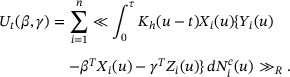
Replacing  by
by  in (3) and taking derivative with respect to γ, we obtain the profile estimating function for γ:
where  is taken as a subinterval of [0, τ] to avoid boundary problems in the theoretical justifications. In practice,
  can be taken to be very close to [0, τ]. Equation
  can be solved explicitly yielding the weighted profile estimator
  , where
The local profile estimator of  is given by
  .
.
2.3 Computational Issues and the Weight Selection
Our estimation procedure uses local smoothing or the local constant method for estimating  . It is known that the local linear estimation technique, cf. Fan and Gijbels (1996), can improve the performance of estimation at boundaries. For the estimation at the inner points, the local linear and local constant estimators are equivalent, with the same asymptotic distributions. As shown in Fan and Gijbels (1996), the boundary effects from the local constant estimator can be reduced by applying the equivalent kernel of the local linear approach.
Following Fan and Gijbels (1996, sections 2.3.1 and 3.2.2), to reduce the estimation bias for  at boundary points, for example,
  , we replace
  by the equivalent kernel to the local linear fit modified for the time-varying coefficient model for longitudinal data, defined by
  , where
  . The equivalent kernel
  is a kernel up to a normalizing constant satisfying the finite sample condition
  . This nice feature works to reduce bias for boundary points similar to the symmetrical kernel for interior points. Because it is simple and faster to use the kernel smoothing, we suggest to estimate
  using the equivalent kernel for the boundary time points, while using the standard kernel for the interior time points. Our simulations show that this adjustment works well.
We proposed a weighted profile least squares estimation method coupled with the EM approach for the semiparametric additive time-varying coefficient model for longitudinal data starting from a possibly censored relevant event. The proposed estimators are consistent and asymptotically normal as long as the weight process  converges in probability to a deterministic function
  . The weight can be selected to improve estimation efficiency, although it is often conveniently taken to be 1. Lin and Carroll (2000) showed that the most efficient estimation of the nonparametric component
  can be achieved by ignoring the within-subject correlation. However, more efficient estimation for the parametric component γ is obtained by using the inverse of true covariance matrix of the longitudinal responses (Lin and Carroll, 2001; Wang et al., 2005). In a simplified situation where the error processes
  are uncorrelated at different times, the optimal weight is inversely proportional to the conditional variance
  of the error process
  (Bickel et al., 1993; Sun et al., 2013; Qi et al., 2017).
We investigated a two-stage estimation procedure for choosing the weight within the framework of the marginal approach that ignores the within-subject correlation. In the first stage, the unit weight function is used to obtain  and
and  . Suppose that
  does not depend on
  , then
  can be consistently estimated by
  ≪
≪ 


 , where
  is the residual of the first stage estimation. In the second stage, the updated estimators
  and
and  are obtained by choosing the weight
  . When
  depends on
  , the optimal weight
  can be estimated using a multivariate kernel estimator (Qi et al., 2017, Web Appendix C). A simulation study is conducted in Section 4.2 to investigate the efficiency of the two-stage estimation procedure.
3 Asymptotic Properties
In this section, we present the asymptotic properties of the proposed estimators. Define 
 ,
,  , and
, and 
 , where
  . Let
. Let  and
and  . Let γ0 and
  be the true values of γ and
  under model (1), respectively. In addition to the conditional independence assumptions and noninformative censoring assumptions stated in Section 2.1, more regularity conditions are given in Condition A in Web Appendix A.
Ying (1989) showed that the consistency and weak convergence of the Kaplan Meier estimation for the distribution of  can be extended to the whole line under Condition (A.7). By Lemma 2 presented in Web Appendix B,
 uniformly in
  . Similar asymptotic results hold for
  and
and  . It follows that
  and
and  converge to
  and
and  uniformly in
  , respectively. These results are the basic building blocks for proving the asymptotic results for
  and
and  .
.
Note that  is the minimizer of
  . In Part (a) of the proof of Theorem 1, we show that
  converges uniformly to a deterministic function of γ that minimizes at
  . The consistency of
  follows by Theorem 5.7 of van der Vaart (1998). By the first-order Taylor expansion of
  at γ0, we have
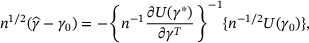
where  is on the line segment between
  and γ0. To prove the asymptotic normality of
  , it is sufficient to prove that
  converges in probability to a nonsingular matrix, and that
  converges in distribution. The convergence of the information matrix can be obtained by applying Lemma 1 in Web Appendix B. We show in Part (b) of the proof of Theorem 1 that
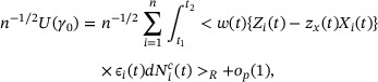
where henceforth we adopt the notation  .
.
The asymptotic properties of  and
and  are summarized as Theorems 1 and 2. Theorems 1 and 2 are proved in Web Appendix B assuming that
  and
and  are independent conditional on
  and both are independent of
  . Web Appendix C provides an outline of the proofs when the conditional hazard function of
  depends on covariates through the Cox model. This model assumption is for the convenience of theoretical development using the existing large sample results for the Cox model with right censored data (Andersen and Gill, 1982). Web Appendix C also discussed possibility of using other failure time regression models to estimate the conditional distribution of left censored event time.
Theorem 1. Under Condition A, we have
- (a)
 as
as  ;
; - (b)

 as
as  , where


 ,
,  .
.
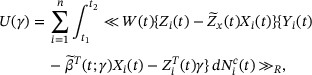
The asymptotic variance of  can be consistently estimated by
  , where
and  .
.
Next we present the asymptotic results for  . First, we introduce a few quantities to be used in the expression of the asymptotic variance of
  . We define
  to be the expected number of sampling points by time t under possibly censored time origin, denoted by
  . Let
. Let 
 be the natural filtration. Then the intensity
  of
of  is given by
  . Hence
  is a
is a  martingale, with predictable variation process
  .
.
Theorem 2. Under Condition A, we have
- (a)
 converges to
  in probability uniformly in
  as
as  ;
; - (b)
For each
 ,
,  as
as  , where
  ,
, 
 . Here
  ,
,  .
.
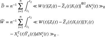
The covariance matrix of  can be estimated by
  , where
  . However, consider the approximation

A more refined variance estimation for  with higher order accuracy can be based on
  , where
This variance estimator is used in the simulations and in the real data application.
4 Simulation Study
We conduct a numerical study to examine the finite sample performance of the proposed methods. Data are simulated using the following semiparametric additive model  :
:

where  ,
,  ,
,  ,
,  is uniformly distributed on [0,1], and
  is a Bernoulli random variable with
  . The error process
  has a normal distribution with mean
  and variance 1 for participant i where
  follows a standard normal distribution.
For participant i,  is generated from a uniform distribution on (0,0.8). The left censoring time
  is generated from a uniform distribution on
  with a and b adjusted to yield a desired percentage
  of left censoring for
  . The first sampling point is set as
  , and the rest of the
  's are generated from a Poisson process
  with intensity rate
  , where
  ,
,  , and
, and  . Let
. Let  be the responses
  at time points
  following model (16). The right censoring time
  is exponentially distributed with the rate parameter adjusted to give a prespecified percentage
  of right censoring (drop-out or administrative censoring at τ) in the time interval [0, τ], which is the probability of
  . We set
  for the time interval
  . The average number of observations in the interval
  per participant is about 4.7. The Epanechnikov kernel
  , and
, and  for the estimating function (9). The local constant kernel
  is used for time points in
  while the equivalent kernel to local linear smoothing is applied for the boundary points in
  . For added protection against boundary bias effects, we consider
  as boundary points in the calculation instead of
  .
.
The performance of the estimator for γ is measured through the bias (Bias), the sample standard error of the estimates (SSE), the estimated standard error of  (ESE), and the coverage probability (CP) of a 95% confidence interval for γ. The performance of the estimator for the jth component
  on the interval
  is evaluated by the square root of average integrated squared error (RASE) defined by
where  is the kth estimate of
  for
for  and N is the number of simulations.
4.1 Simulation Study Using Unit Weight
First, we consider four simulation settings to demonstrate the validity and advantage of the proposed method in handling the censored time origin using unit weight  . The first three settings show the performances of the proposed estimators with
  , and 50% of left censoring for
  . The fourth setting compares the performances of the proposed estimators with the naive version of the approach that ignores the censored time origin (or
  ) by mistreating
  as the measurement times since the actual time origin and
  as the response at
  .
.
For sample sizes  , 300, and 500, and bandwidths
  , 0.4, and 0.5, Table 1 shows results based on 500 simulations. The biases of
  are small, and the sample standard errors of
  are close to the estimated standard errors. Both standard errors decrease as the sample size increases, and they decrease with the left censoring percentage
  . The coverage probabilities of
  are close to their 0.95 nominal level. The
  ,
,  , decrease as sample size increases. The RASEs for
  ,
,  , also increase as
  increases. The values of SSE and ESE for
  are similar for the three different bandwidth choices. But
  and
and  become smaller as bandwidth increases.
Summary statistics for the estimators  and
and  under model (16) with
  left censoring and 30% right censoring. Each entry is based on 500 simulations
 | n | h | Bias | SSE | ESE | CP | RASE | RASE |
|---|---|---|---|---|---|---|---|---|
| 0% | 200 | 0.3 | 0.0075 | 0.1963 | 0.1886 | 0.938 | 0.3798 | 0.6312 |
| 0.4 | 0.0078 | 0.1958 | 0.1893 | 0.940 | 0.3444 | 0.5742 | ||
| 0.5 | 0.0080 | 0.1952 | 0.1900 | 0.938 | 0.3194 | 0.5370 | ||
| 300 | 0.3 | −0.0030 | 0.1640 | 0.1552 | 0.940 | 0.3076 | 0.5157 | |
| 0.4 | −0.0030 | 0.1637 | 0.1556 | 0.938 | 0.2798 | 0.4688 | ||
| 0.5 | −0.0028 | 0.1636 | 0.1559 | 0.940 | 0.2588 | 0.4359 | ||
| 500 | 0.3 | 0.0002 | 0.1184 | 0.1212 | 0.950 | 0.2370 | 0.4048 | |
| 0.4 | 0.0000 | 0.1181 | 0.1214 | 0.950 | 0.2160 | 0.3738 | ||
| 0.5 | 0.0000 | 0.1181 | 0.1216 | 0.952 | 0.2005 | 0.3571 | ||
| 20% | 200 | 0.3 | 0.0003 | 0.1990 | 0.1891 | 0.930 | 0.3961 | 0.6778 |
| 0.4 | 0.0005 | 0.1979 | 0.1899 | 0.932 | 0.3559 | 0.6091 | ||
| 0.5 | 0.0005 | 0.1973 | 0.1903 | 0.938 | 0.3295 | 0.5670 | ||
| 300 | 0.3 | −0.0049 | 0.1650 | 0.1554 | 0.926 | 0.3242 | 0.5436 | |
| 0.4 | −0.0048 | 0.1648 | 0.1558 | 0.928 | 0.2928 | 0.4918 | ||
| 0.5 | −0.0046 | 0.1648 | 0.1562 | 0.930 | 0.2713 | 0.4587 | ||
| 500 | 0.3 | 0.0010 | 0.1164 | 0.1212 | 0.958 | 0.2480 | 0.4293 | |
| 0.4 | 0.0013 | 0.1164 | 0.1215 | 0.960 | 0.2234 | 0.3922 | ||
| 0.5 | 0.0013 | 0.1164 | 0.1217 | 0.960 | 0.2069 | 0.3713 | ||
| 50% | 200 | 0.3 | 0.0013 | 0.2005 | 0.1899 | 0.934 | 0.4474 | 0.7841 |
| 0.4 | 0.0010 | 0.1996 | 0.1911 | 0.936 | 0.3928 | 0.6921 | ||
| 0.5 | 0.0011 | 0.1992 | 0.1917 | 0.936 | 0.3584 | 0.6315 | ||
| 300 | 0.3 | −0.0050 | 0.1663 | 0.1563 | 0.922 | 0.3707 | 0.6415 | |
| 0.4 | −0.0045 | 0.1663 | 0.1571 | 0.926 | 0.3265 | 0.5677 | ||
| 0.5 | −0.0042 | 0.1666 | 0.1575 | 0.926 | 0.2975 | 0.5157 | ||
| 500 | 0.3 | 0.0021 | 0.1170 | 0.1222 | 0.962 | 0.2820 | 0.5166 | |
| 0.4 | 0.0023 | 0.1168 | 0.1226 | 0.964 | 0.2486 | 0.4630 | ||
| 0.5 | 0.0025 | 0.1167 | 0.1228 | 0.960 | 0.2273 | 0.4237 |
| n | h | Bias | SSE | ESE | CP | RASE | RASE |
|---|---|---|---|---|---|---|---|---|
| 0% | 200 | 0.3 | 0.0075 | 0.1963 | 0.1886 | 0.938 | 0.3798 | 0.6312 |
| 0.4 | 0.0078 | 0.1958 | 0.1893 | 0.940 | 0.3444 | 0.5742 | ||
| 0.5 | 0.0080 | 0.1952 | 0.1900 | 0.938 | 0.3194 | 0.5370 | ||
| 300 | 0.3 | −0.0030 | 0.1640 | 0.1552 | 0.940 | 0.3076 | 0.5157 | |
| 0.4 | −0.0030 | 0.1637 | 0.1556 | 0.938 | 0.2798 | 0.4688 | ||
| 0.5 | −0.0028 | 0.1636 | 0.1559 | 0.940 | 0.2588 | 0.4359 | ||
| 500 | 0.3 | 0.0002 | 0.1184 | 0.1212 | 0.950 | 0.2370 | 0.4048 | |
| 0.4 | 0.0000 | 0.1181 | 0.1214 | 0.950 | 0.2160 | 0.3738 | ||
| 0.5 | 0.0000 | 0.1181 | 0.1216 | 0.952 | 0.2005 | 0.3571 | ||
| 20% | 200 | 0.3 | 0.0003 | 0.1990 | 0.1891 | 0.930 | 0.3961 | 0.6778 |
| 0.4 | 0.0005 | 0.1979 | 0.1899 | 0.932 | 0.3559 | 0.6091 | ||
| 0.5 | 0.0005 | 0.1973 | 0.1903 | 0.938 | 0.3295 | 0.5670 | ||
| 300 | 0.3 | −0.0049 | 0.1650 | 0.1554 | 0.926 | 0.3242 | 0.5436 | |
| 0.4 | −0.0048 | 0.1648 | 0.1558 | 0.928 | 0.2928 | 0.4918 | ||
| 0.5 | −0.0046 | 0.1648 | 0.1562 | 0.930 | 0.2713 | 0.4587 | ||
| 500 | 0.3 | 0.0010 | 0.1164 | 0.1212 | 0.958 | 0.2480 | 0.4293 | |
| 0.4 | 0.0013 | 0.1164 | 0.1215 | 0.960 | 0.2234 | 0.3922 | ||
| 0.5 | 0.0013 | 0.1164 | 0.1217 | 0.960 | 0.2069 | 0.3713 | ||
| 50% | 200 | 0.3 | 0.0013 | 0.2005 | 0.1899 | 0.934 | 0.4474 | 0.7841 |
| 0.4 | 0.0010 | 0.1996 | 0.1911 | 0.936 | 0.3928 | 0.6921 | ||
| 0.5 | 0.0011 | 0.1992 | 0.1917 | 0.936 | 0.3584 | 0.6315 | ||
| 300 | 0.3 | −0.0050 | 0.1663 | 0.1563 | 0.922 | 0.3707 | 0.6415 | |
| 0.4 | −0.0045 | 0.1663 | 0.1571 | 0.926 | 0.3265 | 0.5677 | ||
| 0.5 | −0.0042 | 0.1666 | 0.1575 | 0.926 | 0.2975 | 0.5157 | ||
| 500 | 0.3 | 0.0021 | 0.1170 | 0.1222 | 0.962 | 0.2820 | 0.5166 | |
| 0.4 | 0.0023 | 0.1168 | 0.1226 | 0.964 | 0.2486 | 0.4630 | ||
| 0.5 | 0.0025 | 0.1167 | 0.1228 | 0.960 | 0.2273 | 0.4237 |
Summary statistics for the estimators and under model (16) with left censoring and 30% right censoring. Each entry is based on 500 simulations
| n | h | Bias | SSE | ESE | CP | RASE | RASE |
|---|---|---|---|---|---|---|---|---|
| 0% | 200 | 0.3 | 0.0075 | 0.1963 | 0.1886 | 0.938 | 0.3798 | 0.6312 |
| 0.4 | 0.0078 | 0.1958 | 0.1893 | 0.940 | 0.3444 | 0.5742 | ||
| 0.5 | 0.0080 | 0.1952 | 0.1900 | 0.938 | 0.3194 | 0.5370 | ||
| 300 | 0.3 | −0.0030 | 0.1640 | 0.1552 | 0.940 | 0.3076 | 0.5157 | |
| 0.4 | −0.0030 | 0.1637 | 0.1556 | 0.938 | 0.2798 | 0.4688 | ||
| 0.5 | −0.0028 | 0.1636 | 0.1559 | 0.940 | 0.2588 | 0.4359 | ||
| 500 | 0.3 | 0.0002 | 0.1184 | 0.1212 | 0.950 | 0.2370 | 0.4048 | |
| 0.4 | 0.0000 | 0.1181 | 0.1214 | 0.950 | 0.2160 | 0.3738 | ||
| 0.5 | 0.0000 | 0.1181 | 0.1216 | 0.952 | 0.2005 | 0.3571 | ||
| 20% | 200 | 0.3 | 0.0003 | 0.1990 | 0.1891 | 0.930 | 0.3961 | 0.6778 |
| 0.4 | 0.0005 | 0.1979 | 0.1899 | 0.932 | 0.3559 | 0.6091 | ||
| 0.5 | 0.0005 | 0.1973 | 0.1903 | 0.938 | 0.3295 | 0.5670 | ||
| 300 | 0.3 | −0.0049 | 0.1650 | 0.1554 | 0.926 | 0.3242 | 0.5436 | |
| 0.4 | −0.0048 | 0.1648 | 0.1558 | 0.928 | 0.2928 | 0.4918 | ||
| 0.5 | −0.0046 | 0.1648 | 0.1562 | 0.930 | 0.2713 | 0.4587 | ||
| 500 | 0.3 | 0.0010 | 0.1164 | 0.1212 | 0.958 | 0.2480 | 0.4293 | |
| 0.4 | 0.0013 | 0.1164 | 0.1215 | 0.960 | 0.2234 | 0.3922 | ||
| 0.5 | 0.0013 | 0.1164 | 0.1217 | 0.960 | 0.2069 | 0.3713 | ||
| 50% | 200 | 0.3 | 0.0013 | 0.2005 | 0.1899 | 0.934 | 0.4474 | 0.7841 |
| 0.4 | 0.0010 | 0.1996 | 0.1911 | 0.936 | 0.3928 | 0.6921 | ||
| 0.5 | 0.0011 | 0.1992 | 0.1917 | 0.936 | 0.3584 | 0.6315 | ||
| 300 | 0.3 | −0.0050 | 0.1663 | 0.1563 | 0.922 | 0.3707 | 0.6415 | |
| 0.4 | −0.0045 | 0.1663 | 0.1571 | 0.926 | 0.3265 | 0.5677 | ||
| 0.5 | −0.0042 | 0.1666 | 0.1575 | 0.926 | 0.2975 | 0.5157 | ||
| 500 | 0.3 | 0.0021 | 0.1170 | 0.1222 | 0.962 | 0.2820 | 0.5166 | |
| 0.4 | 0.0023 | 0.1168 | 0.1226 | 0.964 | 0.2486 | 0.4630 | ||
| 0.5 | 0.0025 | 0.1167 | 0.1228 | 0.960 | 0.2273 | 0.4237 |
Table 2 presents results for estimation of γ and  with the approach that ignores the censored time origin. It shows that
  ,
,  , increase dramatically compared to the corresponding results of the proposed estimators in Table 1 that account for the censored time origin. Table 2 also shows that there is little bias in the estimation of the constant effect γ when the censored time origin issue is ignored. Table 3 gives a side-by-side comparison of the proposed estimator for
  versus the approach that misplaces the time origin under 50% left censoring in the presence (
 ) and absence (
 ) of right censoring.
Summary statistics of estimation of γ and  under model (16) with misplaced time origin under 50% left censoring and 30% right censoring. Each entry is based on 500 simulations
 | n | h | Bias | SSE | ESE | CP | RASE | RASE |
|---|---|---|---|---|---|---|---|---|
| 50% | 200 | 0.3 | −0.0001 | 0.2341 | 0.2231 | 0.932 | 0.5742 | 1.5619 |
| 0.4 | −0.0007 | 0.2339 | 0.2240 | 0.934 | 0.5477 | 1.5296 | ||
| 0.5 | −0.0009 | 0.2336 | 0.2246 | 0.936 | 0.5265 | 1.4946 | ||
| 300 | 0.3 | −0.0055 | 0.2015 | 0.1847 | 0.920 | 0.5355 | 1.5214 | |
| 0.4 | −0.0056 | 0.2014 | 0.1853 | 0.926 | 0.5171 | 1.4991 | ||
| 0.5 | −0.0058 | 0.2018 | 0.1856 | 0.924 | 0.5007 | 1.4689 | ||
| 500 | 0.3 | −0.0013 | 0.1469 | 0.1444 | 0.936 | 0.4809 | 1.4537 | |
| 0.4 | −0.0013 | 0.1467 | 0.1446 | 0.934 | 0.4695 | 1.4396 | ||
| 0.5 | −0.0014 | 0.1465 | 0.1448 | 0.940 | 0.4579 | 1.4168 |
| n | h | Bias | SSE | ESE | CP | RASE | RASE |
|---|---|---|---|---|---|---|---|---|
| 50% | 200 | 0.3 | −0.0001 | 0.2341 | 0.2231 | 0.932 | 0.5742 | 1.5619 |
| 0.4 | −0.0007 | 0.2339 | 0.2240 | 0.934 | 0.5477 | 1.5296 | ||
| 0.5 | −0.0009 | 0.2336 | 0.2246 | 0.936 | 0.5265 | 1.4946 | ||
| 300 | 0.3 | −0.0055 | 0.2015 | 0.1847 | 0.920 | 0.5355 | 1.5214 | |
| 0.4 | −0.0056 | 0.2014 | 0.1853 | 0.926 | 0.5171 | 1.4991 | ||
| 0.5 | −0.0058 | 0.2018 | 0.1856 | 0.924 | 0.5007 | 1.4689 | ||
| 500 | 0.3 | −0.0013 | 0.1469 | 0.1444 | 0.936 | 0.4809 | 1.4537 | |
| 0.4 | −0.0013 | 0.1467 | 0.1446 | 0.934 | 0.4695 | 1.4396 | ||
| 0.5 | −0.0014 | 0.1465 | 0.1448 | 0.940 | 0.4579 | 1.4168 |
Summary statistics of estimation of γ and under model (16) with misplaced time origin under 50% left censoring and 30% right censoring. Each entry is based on 500 simulations
| n | h | Bias | SSE | ESE | CP | RASE | RASE |
|---|---|---|---|---|---|---|---|---|
| 50% | 200 | 0.3 | −0.0001 | 0.2341 | 0.2231 | 0.932 | 0.5742 | 1.5619 |
| 0.4 | −0.0007 | 0.2339 | 0.2240 | 0.934 | 0.5477 | 1.5296 | ||
| 0.5 | −0.0009 | 0.2336 | 0.2246 | 0.936 | 0.5265 | 1.4946 | ||
| 300 | 0.3 | −0.0055 | 0.2015 | 0.1847 | 0.920 | 0.5355 | 1.5214 | |
| 0.4 | −0.0056 | 0.2014 | 0.1853 | 0.926 | 0.5171 | 1.4991 | ||
| 0.5 | −0.0058 | 0.2018 | 0.1856 | 0.924 | 0.5007 | 1.4689 | ||
| 500 | 0.3 | −0.0013 | 0.1469 | 0.1444 | 0.936 | 0.4809 | 1.4537 | |
| 0.4 | −0.0013 | 0.1467 | 0.1446 | 0.934 | 0.4695 | 1.4396 | ||
| 0.5 | −0.0014 | 0.1465 | 0.1448 | 0.940 | 0.4579 | 1.4168 |
Side-by-side comparison of the proposed estimator for  under model (16) with the approach that misplaces the time origin under 50% left censoring and
  right censoring. Each entry is based on 500 simulations
RASE( ) ) | RASE( ) ) | |||||
|---|---|---|---|---|---|---|
| Proposed | Misplaced | Proposed | Misplaced | |||
 | n | h | method | origin | method | origin |
| 0% | 200 | 0.3 | 0.4078 | 0.5410 | 0.7111 | 1.5325 |
| 0.4 | 0.3557 | 0.5207 | 0.6246 | 1.5081 | ||
| 0.5 | 0.3231 | 0.5033 | 0.5683 | 1.4757 | ||
| 300 | 0.3 | 0.3302 | 0.5084 | 0.5762 | 1.4941 | |
| 0.4 | 0.2903 | 0.4951 | 0.5100 | 1.4791 | ||
| 0.5 | 0.2654 | 0.4818 | 0.4650 | 1.4528 | ||
| 500 | 0.3 | 0.2528 | 0.4686 | 0.4642 | 1.4379 | |
| 0.4 | 0.2230 | 0.4605 | 0.4170 | 1.4294 | ||
| 0.5 | 0.2042 | 0.4505 | 0.3829 | 1.4094 | ||
| 30% | 200 | 0.3 | 0.4474 | 0.5742 | 0.7841 | 1.5619 |
| 0.4 | 0.3928 | 0.5477 | 0.6921 | 1.5296 | ||
| 0.5 | 0.3584 | 0.5265 | 0.6315 | 1.4946 | ||
| 300 | 0.3 | 0.3707 | 0.5355 | 0.6415 | 1.5214 | |
| 0.4 | 0.3265 | 0.5171 | 0.5677 | 1.4991 | ||
| 0.5 | 0.2975 | 0.5007 | 0.5157 | 1.4689 | ||
| 500 | 0.3 | 0.2820 | 0.4809 | 0.5166 | 1.4537 | |
| 0.4 | 0.2486 | 0.4695 | 0.4630 | 1.4396 | ||
| 0.5 | 0.2273 | 0.4579 | 0.4237 | 1.4168 | ||
| RASE() | RASE() | |||||
|---|---|---|---|---|---|---|
| Proposed | Misplaced | Proposed | Misplaced | |||
| n | h | method | origin | method | origin |
| 0% | 200 | 0.3 | 0.4078 | 0.5410 | 0.7111 | 1.5325 |
| 0.4 | 0.3557 | 0.5207 | 0.6246 | 1.5081 | ||
| 0.5 | 0.3231 | 0.5033 | 0.5683 | 1.4757 | ||
| 300 | 0.3 | 0.3302 | 0.5084 | 0.5762 | 1.4941 | |
| 0.4 | 0.2903 | 0.4951 | 0.5100 | 1.4791 | ||
| 0.5 | 0.2654 | 0.4818 | 0.4650 | 1.4528 | ||
| 500 | 0.3 | 0.2528 | 0.4686 | 0.4642 | 1.4379 | |
| 0.4 | 0.2230 | 0.4605 | 0.4170 | 1.4294 | ||
| 0.5 | 0.2042 | 0.4505 | 0.3829 | 1.4094 | ||
| 30% | 200 | 0.3 | 0.4474 | 0.5742 | 0.7841 | 1.5619 |
| 0.4 | 0.3928 | 0.5477 | 0.6921 | 1.5296 | ||
| 0.5 | 0.3584 | 0.5265 | 0.6315 | 1.4946 | ||
| 300 | 0.3 | 0.3707 | 0.5355 | 0.6415 | 1.5214 | |
| 0.4 | 0.3265 | 0.5171 | 0.5677 | 1.4991 | ||
| 0.5 | 0.2975 | 0.5007 | 0.5157 | 1.4689 | ||
| 500 | 0.3 | 0.2820 | 0.4809 | 0.5166 | 1.4537 | |
| 0.4 | 0.2486 | 0.4695 | 0.4630 | 1.4396 | ||
| 0.5 | 0.2273 | 0.4579 | 0.4237 | 1.4168 | ||
Side-by-side comparison of the proposed estimator for under model (16) with the approach that misplaces the time origin under 50% left censoring and right censoring. Each entry is based on 500 simulations
| RASE() | RASE() | |||||
|---|---|---|---|---|---|---|
| Proposed | Misplaced | Proposed | Misplaced | |||
| n | h | method | origin | method | origin |
| 0% | 200 | 0.3 | 0.4078 | 0.5410 | 0.7111 | 1.5325 |
| 0.4 | 0.3557 | 0.5207 | 0.6246 | 1.5081 | ||
| 0.5 | 0.3231 | 0.5033 | 0.5683 | 1.4757 | ||
| 300 | 0.3 | 0.3302 | 0.5084 | 0.5762 | 1.4941 | |
| 0.4 | 0.2903 | 0.4951 | 0.5100 | 1.4791 | ||
| 0.5 | 0.2654 | 0.4818 | 0.4650 | 1.4528 | ||
| 500 | 0.3 | 0.2528 | 0.4686 | 0.4642 | 1.4379 | |
| 0.4 | 0.2230 | 0.4605 | 0.4170 | 1.4294 | ||
| 0.5 | 0.2042 | 0.4505 | 0.3829 | 1.4094 | ||
| 30% | 200 | 0.3 | 0.4474 | 0.5742 | 0.7841 | 1.5619 |
| 0.4 | 0.3928 | 0.5477 | 0.6921 | 1.5296 | ||
| 0.5 | 0.3584 | 0.5265 | 0.6315 | 1.4946 | ||
| 300 | 0.3 | 0.3707 | 0.5355 | 0.6415 | 1.5214 | |
| 0.4 | 0.3265 | 0.5171 | 0.5677 | 1.4991 | ||
| 0.5 | 0.2975 | 0.5007 | 0.5157 | 1.4689 | ||
| 500 | 0.3 | 0.2820 | 0.4809 | 0.5166 | 1.4537 | |
| 0.4 | 0.2486 | 0.4695 | 0.4630 | 1.4396 | ||
| 0.5 | 0.2273 | 0.4579 | 0.4237 | 1.4168 | ||
Figure 2 shows the average estimates of  based on 500 simulations under the four simulation settings described above. Figure 2(a)–(c) plots average estimates based on the proposed method corresponding to 0%, 20%, and 50% left censoring for
  , and Figure 2(d) corresponds to the fourth case. Figure 2(a)–(c) shows that the biases are small, thus the estimated curves fit the true curve quite well. In contrast, there are large biases and an obvious time shift in the estimated covariate effect for
  in Figure 2(d).
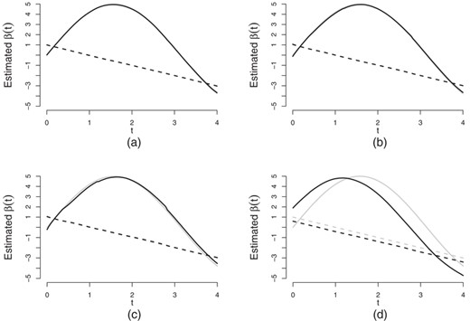
Averages of the estimates for  and
and  for
for  ,
,  and 30% right censoring based on 500 simulations. The solid black lines are for
  and the dashed black lines are for
  . (a)–(c) The biases in the cases of 0%, 20%, and 50% left censoring rate of
  , respectively. (d) The results in the case of misplaced time origin by ignoring
Figure 3 shows standard errors of  and
and  based on 500 simulations under the four simulation settings. Figure 3(a)–(d) plots results under the four simulation settings. In all four plots, the sample standard error curves are quite close to the estimated standard error curve. In the first three cases, large variations for time near zero are typical for the local linear approach near the boundaries; see page 73 of Fan and Gijbels (1996). The fourth case in Figure 3(d) does not have large variation near zero as the new time zero is shifted from a time point that is of duration
  after the actual time origin for ith subject,
  .
.
Sample and estimated standard errors of the estimates for  and
and  for
for  ,
,  and 30% right censoring based on 500 simulations. The solid lines are for
  and the dashed lines are for
  . The gray lines are the estimated standard error and the black ones are the sample standard error. (a)–(c) The results in the cases of 0%, 20%, and 50% left censoring rate of
  , respectively. (d) The results in the case of misplaced time origin by ignoring
Figure 4 shows the coverage probabilities of 95% pointwise confidence intervals for  and
and  for
for  based on 500 simulations under the four simulation settings. Figure 4(a)–(c) shows that the proposed estimators have accurate coverage probabilities close to the 0.95 nominal level except for time near zero, while Figure 4(d) shows very poor coverage probabilities for both
  and
and  for the approach that ignores the censored time origin.
Coverage probabilities of 95% pointwise confidence intervals for  and
and  for
for  ,
,  and 30% right censoring based on 500 simulations. The solid lines are the coverage probabilities for
  and the dashed lines are for
  . (a)–(c) The coverage probabilities of 95% pointwise confidence intervals in the cases of 0%, 20% and 50% left censoring rate of
  , respectively. (d) The results in the case of misplaced time origin by ignoring
An additional simulation study is conducted in Web Appendix D when the conditional hazard function of  depends on the baseline covariates through the Cox model. The simulation results presented in Web Tables 1–3 and Web Figures 1–3 show that the theory and methods work well for the Cox model.
4.2 Simulation Study Using the Estimated Weight
A simulation study is conducted to evaluate the efficiency gain of the two-stage estimation procedure. We consider four different error models for  . In Error Model I,
  is a normal distribution with mean
  and variance 1 conditional on the ith subject, and
  is N(0, 1). In Error Model II,
  has a normal distribution with mean
  and variance of
  conditional on the ith subject, and
  is N(0, 0.52). Error Model III is same as for Error Model II except for
  from N(0, 0.32). In Error Model IV,
  is a Gaussian process with mean 0 and variance
  , and
, and  and
and  are independent for
  . Errors
  and
and  for
for  are dependent under both Error Models I, II, and III, but independent under Error Models IV. Variance
  of error
  is time-varying under Error Models II–IV, but constant under Error Models I. The second-stage estimator is obtained by using the estimated weight
  where
where  is given in Section 2.3.
Define the empirical relative efficiency (Eff) of the weighted estimator  to
to  as
as  . The efficiency gain depends on the distribution of error process
  . Table 4 shows the simulation results on performance of the second-stage estimator and its empirical relative efficiency. Overall empirical relative efficiency varies in the range of 1 and 1.35. The amount of the efficiency gain is not observed when variance of
  is constant. The second-stage estimator is most efficient when errors
  at different time points are not correlated. The efficiency gain is less obvious when errors
  are correlated. The simulation study also shows that there is no clear efficiency gain of
  over
over  for all error models.
The empirical relative efficiency Eff(γ) of the two-stage estimator using the estimated weight to the estimator using unit weight under model (16) with 20% left censoring and 30% right censoring, n = 200, 300, 500 and  . Each entry is based on 500 simulations
| Unit Weight | Estimated Weight | ||||||||
|---|---|---|---|---|---|---|---|---|---|
| n | Bias | SSE | ESE | CP | Bias | SSE | ESE | CP | Eff(γ) |
| Error Model I | |||||||||
| 200 | 0.0005 | 0.1979 | 0.1899 | 0.932 | 0.0006 | 0.1984 | 0.1875 | 0.932 | 0.9972 |
| 300 | −0.0048 | 0.1648 | 0.1558 | 0.928 | −0.0050 | 0.1650 | 0.1545 | 0.928 | 0.9988 |
| 500 | 0.0013 | 0.1164 | 0.1215 | 0.960 | 0.0012 | 0.1162 | 0.1208 | 0.960 | 1.0017 |
| Error Model II | |||||||||
| 200 | 0.0001 | 0.1282 | 0.1263 | 0.952 | 0.0006 | 0.1197 | 0.1143 | 0.940 | 1.0707 |
| 300 | −0.0041 | 0.1070 | 0.1035 | 0.940 | −0.0021 | 0.0992 | 0.0939 | 0.928 | 1.0789 |
| 500 | 0.0000 | 0.0774 | 0.0803 | 0.954 | 0.0009 | 0.0706 | 0.0733 | 0.964 | 1.0959 |
| Error Model III | |||||||||
| 200 | −0.0007 | 0.1066 | 0.1071 | 0.958 | 0.0000 | 0.0918 | 0.0896 | 0.956 | 1.1612 |
| 300 | −0.0036 | 0.0901 | 0.0876 | 0.940 | −0.0013 | 0.0773 | 0.0732 | 0.924 | 1.1665 |
| 500 | −0.0003 | 0.0658 | 0.0679 | 0.956 | 0.0007 | 0.0550 | 0.0570 | 0.964 | 1.1970 |
| Error Model IV | |||||||||
| 200 | −0.0018 | 0.0929 | 0.0954 | 0.954 | −0.0009 | 0.0709 | 0.0715 | 0.950 | 1.3100 |
| 300 | −0.0028 | 0.0794 | 0.0779 | 0.948 | −0.0006 | 0.0602 | 0.0580 | 0.932 | 1.3187 |
| 500 | −0.0009 | 0.0597 | 0.0603 | 0.950 | 0.0003 | 0.0443 | 0.0451 | 0.958 | 1.3481 |
The empirical relative efficiency Eff(γ) of the two-stage estimator using the estimated weight to the estimator using unit weight under model (16) with 20% left censoring and 30% right censoring, n = 200, 300, 500 and . Each entry is based on 500 simulations
| Unit Weight | Estimated Weight | ||||||||
|---|---|---|---|---|---|---|---|---|---|
| n | Bias | SSE | ESE | CP | Bias | SSE | ESE | CP | Eff(γ) |
| Error Model I | |||||||||
| 200 | 0.0005 | 0.1979 | 0.1899 | 0.932 | 0.0006 | 0.1984 | 0.1875 | 0.932 | 0.9972 |
| 300 | −0.0048 | 0.1648 | 0.1558 | 0.928 | −0.0050 | 0.1650 | 0.1545 | 0.928 | 0.9988 |
| 500 | 0.0013 | 0.1164 | 0.1215 | 0.960 | 0.0012 | 0.1162 | 0.1208 | 0.960 | 1.0017 |
| Error Model II | |||||||||
| 200 | 0.0001 | 0.1282 | 0.1263 | 0.952 | 0.0006 | 0.1197 | 0.1143 | 0.940 | 1.0707 |
| 300 | −0.0041 | 0.1070 | 0.1035 | 0.940 | −0.0021 | 0.0992 | 0.0939 | 0.928 | 1.0789 |
| 500 | 0.0000 | 0.0774 | 0.0803 | 0.954 | 0.0009 | 0.0706 | 0.0733 | 0.964 | 1.0959 |
| Error Model III | |||||||||
| 200 | −0.0007 | 0.1066 | 0.1071 | 0.958 | 0.0000 | 0.0918 | 0.0896 | 0.956 | 1.1612 |
| 300 | −0.0036 | 0.0901 | 0.0876 | 0.940 | −0.0013 | 0.0773 | 0.0732 | 0.924 | 1.1665 |
| 500 | −0.0003 | 0.0658 | 0.0679 | 0.956 | 0.0007 | 0.0550 | 0.0570 | 0.964 | 1.1970 |
| Error Model IV | |||||||||
| 200 | −0.0018 | 0.0929 | 0.0954 | 0.954 | −0.0009 | 0.0709 | 0.0715 | 0.950 | 1.3100 |
| 300 | −0.0028 | 0.0794 | 0.0779 | 0.948 | −0.0006 | 0.0602 | 0.0580 | 0.932 | 1.3187 |
| 500 | −0.0009 | 0.0597 | 0.0603 | 0.950 | 0.0003 | 0.0443 | 0.0451 | 0.958 | 1.3481 |
5 Analysis of Step Study
Step study was a multicenter, double-blind, randomized, placebo-controlled preventive HIV vaccine efficacy trial conducted in North America, the Caribbean, South America, and Australia from 2004 to 2009 (Buchbinder et al., 2008; Fitzgerald et al., 2011; Duerr et al., 2012). A co-primary objective of the study was to determine whether the MRKAd5 HIV gag/pol/nef vaccine, which elicits T cell immune responses to HIV proteins through delivery of the gag, pol, and nef HIV genes to the immune system by the adenovirus type 5 (Ad5) common cold vector, is capable of controlling HIV replication among participants who acquired HIV infection after vaccination. Three thousand HIV-1 negative participants at high risk of HIV infection and with ages between 18 and 45 were enrolled and randomly assigned to receive vaccine or placebo in 1:1 allocation, stratified by sex, study site, and anti-Ad5 neutralizing antibody titer at baseline.
Of the 3000 participants, 174 acquired HIV infection during the trial, 159 of which were male and 15 female. As females comprised only <10% of the sample, we analyze the males only. Study participants received antibody (Ab)-based HIV diagnostic ELISA tests at periodic study visits at Weeks 12, 52, and every six months thereafter through 5 years. Participants with a positive ELISA test had HIV infection confirmed by an antigen-based HIV-specific RNA PCR test. Moreover, for all confirmed HIV infected participants, a “look-back” procedure was applied wherein all earlier available blood samples going back in time were tested for HIV infection using the more sensitive RNA PCR test. The antibody tests used in Step have near-perfect sensitivity to detect HIV infections starting 4 weeks after HIV acquisition, but miss HIV infections before that, whereas the RNA PCR tests have near-perfect sensitivity starting about a week after HIV acquisition. Let  be the time of the latest negative Ab- test result,
  the first positive Ab+ test result, and
  the actual HIV acquisition time. Based on the HIV testing algorithm, each infected participant was classified into one of two groups, defined by whether the earliest HIV positive sample was (Ab+, PCR+) or (Ab-, PCR+). The (Ab+, PCR+) group has
  such that
  and
and  is left censored (Figure 1a), and the (Ab-, PCR+) group has
  and
and  such that
  is observed (Figure 1b). The left censoring rate for
  is 70.4%.
At the time of a participant's first antibody-based positive HIV infection diagnosis ( ), 18 post-infection visits were scheduled at weeks 0, 1, 2, 8, 12, 26 and every 26 weeks thereafter through week 338. However, the actual dates of visits vary. We define
  as the time from
  to the jth visit for the ith infected participant. At each study visit, HIV viral load
  was measured. A participant is considered censored once he starts antiretroviral therapy (ART), which interferes with the assessment of vaccine effects on viral load and other biomarkers of interest. The censoring time
  is the time from
  to ART initiation, study drop-out, or the end of follow-up, whichever comes first. The right censoring rate of
  was 69.8%.
The data for analysis includes 159 participants (97 vaccine group, 62 placebo group) with 785 visits from HIV infection diagnosis and prior to ART initiation. One hundred and twenty-two participants were in North America or Australia and the rest were in the Caribbean or South America. Information was available on whether the participants were fully adherent to vaccinations and on baseline anti-Ad5 neutralizing antibody titer (Ad5 titer), each of which affect the T cell response to the vaccine and hence could associate with the viral load response. A spaghetti plot of the raw viral load data with one line for each participant by vaccination status and the study region is given in Web Figure 4 in Web Appendix F. We investigate the effect of MRKAd5 HIV-1 gag/pol/nef vaccine versus placebo on longitudinal HIV viral loads among the 159 HIV infected men. With  , the logarithm (log10) of HIV viral load at time t in years, we analyzed the data with the following model:

where  is the treatment indicator (
 if participant i was assigned vaccine and 0 if placebo),
  is the study site indicator (
 if North America or Australia and 0 otherwise),
  is the natural logarithm of baseline Ad5 titer, and
  is the per-protocol indicator (
 if participant i was fully adherent to vaccinations and 0 otherwise).
We choose  years since there are very few observations after
  and
and  . The Kaplan–Meier estimator is used to estimate distribution of
  since the covariates in model (18) are not significant with large p-values in fitting the Cox model. Figure 5 shows the plot of the Kaplan–Meier estimator
  . We let
  for
for  as the smallest uncensored
  is 0.1397 and the smallest value of
  is 0.0493.
Kaplan–Meier estimator of the distribution function of the time from actual HIV acquisition to the first positive Elisa confirmed by Western Blot or RNA for male HIV infected cases in Step trial
We select bandwidth using the formula  , where
  . Here
  is the sample variance of
  , for
, for  and each participant i, and
  is the sample variance of
  . Some discussions on bandwidth choice are given in Web Appendix E. With
  , the bandwidth choice is
  . The estimates of γ1, γ2, and γ3 using unit weight are 0.0241, −0.0127, and −0.0124, with standard error 0.0406, 0.1935, and 0.1573, respectively. The results indicate no significant associations of baseline Ad5 titer, study site, or per-protocol status with the HIV viral load level. The estimates of time-varying effects with 95% pointwise confidence intervals are shown in Figure 6. Figure 6(b) suggests that there is a nonsignificant vaccine effect to reduce viral load after infection. However, the vaccine group tends to have lower viral load than the placebo group and the benefit increases over time.
Analysis of HIV viral load level for the male HIV infected cases in Step trial with model (18). (a) The estimate of the intercept  and its 95% pointwise confidence interval. (b) The estimated effect
  of the vaccine and its 95% pointwise confidence interval. The solid curves are the point estimates and the dashed curves are the confidence intervals
The two-stage estimation procedure with the estimated weight is applied to the analysis of Step study. The results of analysis using the estimated weight are similar and are presented in Web Appendix F.
6 Concluding Remarks
This paper investigated the semiparametric additive time-varying coefficient model for longitudinal data starting from a possibly censored relevant event. The developed method can be applied to assess the HIV vaccine effect on the post HIV infection longitudinal biomarkers such as HIV viral load level since the time of infection. However, the exact time of infection can be censored. The censorship status can be determined by an HIV antibody test followed by a more sensitive antigen-based HIV-specific PCR assay, or by an expanded set of HIV diagnostic assays with varying sensitivity properties (Grebe et al., 2019) and/or sequence diversification molecular clock models (Giorgi et al., 2010; Rossenkhan et al., 2019). The time from HIV acquisition to first HIV antibody positive test is subject to left censoring and its distribution can be estimated based on the Kaplan–Meier estimator or a failure time regression model such as the Cox model. We used the expectation maximization approach to deal with the censored time origin and developed the weighted profile least squares estimation procedure. The nonparametric kernel smoothing method was employed to estimate time-varying covariate effects. We investigated the asymptotic properties of both the parametric and nonparametric estimators and proposed consistent variance estimators.
Our simulation study showed that the proposed estimators work well with small biases and satisfying coverage probabilities for different levels of left censoring and moderate sample sizes while substantial bias was incurred for estimation of time-varying effects when misplacing the time origin by ignoring left censoring. The method was applied to analyze the male HIV infected cases from Step study, suggesting a borderline significant vaccine effect to lower viral load after infection by about a half to three-quarters of a log (base 10) during the period beyond 1.5 years post HIV acquisition. This result should be interpreted with caution given the potential for post-randomization selection bias, which could occur if there are baseline factors not adjusted for in the analysis that predict both viral load and the vaccine effect on HIV acquisition (Shepherd et al., 2006).
As with most statistical modeling, the application of the proposed method should be accompanied by model assessment. Web Figure 5 shows a scatter plot of residuals of the participants with  for the Step study application. The residual plot is approximately centered around 0 between −2 and 2, which indicates the model fits the data reasonably well. However, it is more desirable to develop formal goodness-of-fit tests to examine the model fitness. The test statistics can be constructed based on certain test processes that are functionals of residual processes. The critical values of the test statistics can be estimated similarly to the technique of Sun et al. (2019). Further work is warranted to understand the empirical and theoretical properties of the tests. Although the development for the censored time origin is based on the semiparametric additive time-varying coefficients model, extensions to the generalized semiparametric regression models of Sun et al. (2013) are possible. The extension can be carried out by applying the EM approach to the expositions of Sun et al. (2013). It would also be interesting to investigate the random mixed-effects model with censored time origin that can be used to estimate subject-specific effects of covariates.
Data Availability Statement
The data that support the findings in this paper are available in the Supporting Information of this article.
Supporting Information
Web Appendices A–F, Tables 1–3, and Figures 1–5 referenced in Sections 2–5 together with the data and computer code are posted online with this paper at the Biometrics website on Wiley Online Library.
Acknowledgments
The authors thank an associate editor and two referees for their valuable comments and suggestions that have greatly improved the paper. This research was partially supported by the National Institutes of Health NIAID [grant number R37 AI054165]. The research of Yanqing Sun was also partially supported by the National Science Foundation [grant numbers DMS-1208978 and DMS-1915829] and the Reassignment of Duties fund provided by the University of North Carolina at Charlotte. We thank the HIV Vaccine Trials Network (HVTN) and Merck for providing the data analyzed in this article. The HVTN is supported through a cooperative agreement with the National Institutes of Health Division of AIDS, grant 5 U01 AI068635. The content is solely the responsibility of the authors and does not necessarily represent the official views of the National Institutes of Health.
