Summary
It is frequently observed in practice that the Wald statistic gives a poor assessment of the statistical significance of a variance component. This paper provides detailed analytic insight into the phenomenon by way of two simple models, which point to an atypical geometry as the source of the aberration. The latter can in principle be checked numerically to cover situations of arbitrary complexity, such as those arising from elaborate forms of blocking in an experimental context, or models for longitudinal or clustered data. The salient point, echoing Dickey (2020), is that a suitable likelihood-ratio test should always be used for the assessment of variance components.
1 Introduction
Faithful representation of a process generating data often entails specification of two or more sources of variability. In an experimental context, simple or elaborate forms of blocking induce a nested or crossed structure within the set of plots. Similar grouping arises in observational studies where, for instance, data may originate from different hospitals, regions or from several family groups, of no direct interest, but likely to generate structured correlation in the outcome.
As in certain other settings, inference based on the likelihood function for the full generative model is typically miscalibrated, sometimes seriously so, and should ideally be based on a suitable marginal or conditional likelihood. In the present context, appropriate preliminary reduction leads to residual maximum likelihood, REML, developed by Patterson & Thompson (1971), and closely connected to marginal likelihood (Bartlett, 1937).
Even when the REML likelihood is used, the Wald test routinely reported in software implementations is frequently found to be ineffectual for detecting components of variance when they are unambiguously present. A typical example occurs in McCullagh (2023, Ch. 4), where the likelihood-ratio statistic is more than eight times as large as the squared Wald ratio. The phenomenon has also been documented by Dickey (2020), who presented examples in which the REML Wald statistic is bounded. In at least one of the examples he considered, the natural estimate of standard error of the REML estimator is proportionate to the REML estimate itself, so that the role of the data in the Wald construction is negligible. The purpose of the present paper is to expose the matter in a form amenable to detailed analytic calculation, thereby revealing dependence on key aspects and indicating other settings in which the same phenomenon is inevitable. The insights of Dickey (2020) are reproduced and elucidated further. The source of the anomalous behaviour is not a failure of distributional approximations obtained under hypothetical regimes of sometimes questionable adequacy, but rather atypical geometry of the REML loglikelihood function, which induces a bounded Wald statistic even under a notional limiting operation in which the likelihood-ratio statistic for testing the same hypothesis is arbitrarily large. We show that a version of the score statistic is subject to the same aberration.
The implications for applied work are consequential, as undetected sources of variability typically result in estimated standard errors for regression coefficient estimators that are deceptively small, and therefore confidence intervals that are misleadingly narrow. The opposite situation can occasionally arise as well. For instance, in a randomized block design, omission of the block factor as a variance component has the effect of increasing the estimated variance of treatment effect estimators.
2 Variance-component models
In a typical variance-component model, the distribution of the response vector is specified by a mean vector in the linear subspace spanned by the columns of the model matrix X, and a covariance matrix Σ in the convex cone
spanned by given matrices , which are positive definite or semidefinite. Usually, is the identity; the remaining matrices may be block factors or structured matrices associated with spatial or temporal dependence.
The residual likelihood is the likelihood function based on the residual , where . Provided that the matrices are linearly independent, the variance components θu may be estimated by maximizing the residual likelihood. In the subsequent discussion, reference to the loglikelihood function and its maximizer means the REML version unless otherwise specified.
There are compelling general arguments, notably invariance and permissibility of asymmetric confidence regions, for basing an assessment of the hypothesis , say, on the likelihood-ratio statistic
where is the maximum likelihood estimator and is the constrained estimator under H0. Nonnegativity of the variance coefficients means that the subset of defined by the constraint is a boundary subcone, with the implication that the likelihood achieves its maximum on the boundary with positive probability, usually one half for sufficiently large sample size (Chernoff, 1954). When an exact F statistic exists, the boundary event occurs whenever . On this event, coincides with and the loglikelihood ratio is exactly zero. Thus, with asymptotic probability one half, Λ = 0; otherwise, its distribution under H0 is under suitable limiting conditions. The realized value of Λ is to be calibrated against this distribution.
The nominal asymptotic variance of is , the (s, s) component of the inverse Fisher information matrix. With asymptotic probability one half, the squared Wald ratio is equal to zero under H0; otherwise, it is asymptotically equivalent to Λ by a standard asymptotic argument. However, it is frequently observed in practice that W2 gives a poor assessment of the statistical significance of the sth variance component, in the sense that it fails to reject H0 even when Λ does so unambiguously at the same significance level. If the likelihood is maximized on the boundary, both W2 and Λ are zero and there is no disagreement. Disagreement can only occur when both are positive, and it is that phenomenon that we address here.
Among the substantial literature on testing variance components is an early contribution by Wald (1947), notable in that it recommends an F test but fails to warn against use of the eponymous statistic in this context. Subsequent contributions have developed nonstandard asymptotic theory for the likelihood-ratio statistic and modifications thereof, relaxing an earlier assumption that the true parameter value belongs to the interior of the parameter space (e.g., Self & Liang, 1987; Geyer, 1994; Vu & Zhou, 1997). While the likelihood-ratio test and its variants have been the focus of theoretical development, common software implementations report Wald statistics as standard, without warning. Dickey (2020) appears to have been the first to emphasize the point at issue. The popularity of Wald-based inference perhaps stems from the convenience of its construction, requiring a single maximum likelihood fit in contrast with two for Λ, which facilitates the presentation of confidence statements.
The analysis of § 3 and § 6 is comparable to that of Dickey (2020), whose derivations cover situations in which the likelihood-ratio test coincides with an exact F test. The two papers illustrate the aberration under study in different ways and § 3.4 provides a comparison and synthesis. Sections 4 and 5 cover situations in which a fruitful formulation in terms of F may be infeasible, but for which the shared anomalous geometry can be checked by direct study of the loglikelihood function. Together, the present paper and that of Dickey (2020) provide a thorough explanation of a phenomenon of broad relevance and scientific consequence.
3 Analysis for a single block factor
3.1 Introduction
We consider in this section a simple Gaussian model with two variance components estimated from the sufficient statistic, which consists of the within-block mean square on f0 degrees of freedom and the between-block mean square on f1 degrees of freedom. Specifically, the outcome is (), where, for an arbitrary block index j, has a Gaussian distribution of mean and covariance matrix . Define, in a standard notation for averaging over suffixes, , and similarly for the double average. The between-block sum of squares
is distributed as , where and, in the usual variance-component parameterization with ,
The within-block sum of squares is distributed independently of the between-block sum of squares, where . The constraint on θ means that the null hypothesis of equality of variances is on the boundary.
In the balanced one-way analysis of the variance structure of the above formulation, the REML loglikelihood is the marginal loglikelihood based on the joint density function of . While numerous generalizations may be considered, the simple version presented here isolates the point at issue in the most incisive form, free of secondary effects that complicate the analysis and interpretation.
3.2 Comparison of Wald and likelihood-ratio statistics
Maximization of without the constraint produces estimators and , where is Fisher’s F ratio, whose distribution depends only on the variance ratio θ. The maximum likelihood estimator has nominal asymptotic variance given by the relevant diagonal component of the inverse Fisher information matrix, namely,
where . The squared Wald statistic for testing θ = 0 is therefore
to be compared with the likelihood-ratio statistic
where the pooled mean square is the maximum likelihood estimator of under the constraint θ = 0.
Although the statistics W2 and Λ are known functions of , simple approximations provide insight into the nature of the aberration described in § 1. A Taylor expansion of W2 and Λ around gives
or, in terms of ,
showing that they agree up to second order in and to first order in Λ, but not beyond. Typically, is large, in which case the ratio is approximately
for small or Λ.
The squared Wald statistic W2 is justified based on standard asymptotic theory for maximum likelihood estimators. First- and second-moment theory suggests three further Wald statistics, for which the same anomalous behaviour is demonstrated in the Supplementary Material. For a similar discussion of two score statistics, see also the Supplementary Material.
In the simplest setting, at least, both W and are monotone functions of the mean-square ratio F, so their distributions are known exactly as a function of the variance-ratio parameter θ. The transformations and are strictly monotone increasing for F > 1, and decreasing for F < 1. The discrepancies described here arise from the standard practice of treating Λ and W2 as if they were asymptotically identical statistics rather than equivalent statistics. The standard practice is justified only if g1 = g2, at least approximately for large samples, which is not the case in typical variance-components models.
One definition of Wald-detectability equates θ to times the estimated standard error of . It can be shown that there does not exist a positive Wald-detectable value in this sense unless the number of blocks is large. It is arguably more natural to compute standard errors under the null, in which case the values at the borderline of Wald detectability are
at the 16% and 2% levels. The corresponding thresholds in terms of F are
With and b = 18, the ratio is approximately 1.864 at and 2.727 at . With the same numbers, and , to be compared with the 16% and 2% critical values of the F distribution on (f1, f0) degrees of freedom, which are 1.625 and 2.818, respectively. Thus, even when standard errors are computed under the null hypothesis, the observed value of the F statistic has to be 17% larger than the 2% critical value of the F distribution in order for the Wald test to reject at the same level. Equivalently, rejection at the 2% level using a Wald statistic with standard errors computed under the null requires an observed value of that is double that necessary for rejection at the same level using an F test. These latter conclusions do not involve any approximations, and are similar and complementary to those of Dickey (2020).
Geometric insight is obtained by noting that the Wald statistic W2 implicitly defines a quadratic approximation to the profile REML loglikelihood function, in a neighbourhood of . Specifically, for fixed θ, the maximum likelihood estimator of is , where and
Write . The quadratic approximation to implicit in the Wald test is
where is and
Since the two functions have the same value at , the discrepancy between the Wald and likelihood-ratio statistics for testing θ = 0 is the difference in y intercepts:
with the expression for Λ in terms of F given by
For F and f1 fixed,
showing that the discrepancy is roughly linear in F for large f0, while for fixed f1 and f0, (4) converges to zero as F approaches unity and is unbounded for F arbitrarily large. Figure 1 graphs and for different values of F.
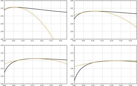
Fig. 1
Graphs of the profile REML loglikelihood function (solid lines) and its quadratic approximation (dashed lines) for , b = 18, and (from top left to bottom right).
3.3 Nonconstant Fisher information and anomalous geometry
From (3), has second derivative
whose value at is
showing that the curvature at the maximum-likelihood point is close to zero for large F, as depicted in Fig. 1. In other words, is arbitrarily well approximated by a horizontal asymptote at in a neighbourhood of for arbitrarily large F. Equation (5) also shows that the discrepancy is attributable to the higher-order derivatives, since there is no error incurred by using in place of in the Taylor series approximation to . The effect of higher-order derivatives is encapsulated to a large extent in the considerable nonconstancy of as a function of θ over the range of interest.
From (1), the ratio of the nominal asymptotic variances of at arbitrary θ and at θ = 0 is , and the range of primary interest is
the upper value being the nominal asymptotic standard deviation of under the null hypothesis, having conditioned on the event that is not on the boundary. Over this range, the asymptotic variance varies by a factor
which is large for typical values of f1. For example, gives a range of approximately .
The motivation for the present paper came from practical examples in McCullagh (2023, Ch. 4), where the Wald statistic was ineffectual at detecting variance components, the absence of which was strongly refuted by a likelihood-ratio test. Dickey (2020) exposed the same phenomenon. His exposition, aimed at practitioners, covers widely used models in the analysis of designed experiments for which exact F and Wald tests are available. The present paper is framed in terms of the loglikelihood-ratio statistic Λ, which is more generally available and points to geometric insights not recoverable from the moment-based Wald constructions. Three instances of the latter are discussed in the Supplementary Material, among which equation (S.1) coincides with equation (2) of Dickey (2020). For cases where F is available, the present paper and that of Dickey provide equivalent explanations from two points of view.
4 Two-sample problem in general scale families
Let Y be a random variable from a scale family with density function , where g is a known, continuous, density function on the positive real line. Let
Then the Fisher information for τ in an independent and identically distributed sample is and that for in a two-sample problem of sizes n0 and n1 is
The squared Wald statistic for testing equality of scale parameters is therefore
where is the estimated ratio . The Wald statistic is bounded in both limits for arbitrarily large or small. Specifically,
The curvature of the profile loglikelihood function at is approximated by the expected Fisher information in the profile loglikelihood. The Fisher information transforms as
where ψ and are two parameterizations and we have used the convention that symbols appearing both as subscripts and superscripts in the same product are summed. The information about θ, having adjusted for estimation of τ0 is therefore, using (6) and (7),
showing that the two-sample problem in general scale families has the same anomalous geometry documented in § 3 for large θ, leading to the discrepancy between the likelihood-ratio and the Wald statistics.
5 Gaussian variance-component model
Consider a variance-component model in which is normal with mean of dimension p < n, and covariance matrix , where is a known matrix function of a vector parameter with . This encompasses the linear model from § 2. The subspace is a group under addition, which implies that, for any matrix with kernel , the normalized residual statistic
is maximal invariant under the affine group with action , with a > 0 and . For distributional calculations, it is convenient to take the columns of U to be an orthonormal basis in , the orthogonal complement of with respect to the standard inner product. In that case and the density function of is
where . At θ = 0, Q is uniformly distributed on the -dimensional unit sphere in . The above exposition hybridizes Kariya (1980) and King (1980).
By construction, distribution (8) does not depend on β or , and inference for θ is conveniently based on the marginal loglikelihood function
closely related to the REML loglikelihood function that uses the marginal distribution of rather than Q. Since the transformation to Q eliminates the nuisance parameter as well as β, analysis based on (9) is more amenable to analytic calculation.
The density function in (8) is relative to a particular orthonormal basis in , and the same basis is embedded in the likelihood function (9) in matrix . The conclusion in (9) is equivalent to equation (3.3) of McCullagh (2009), which evades the problem of selecting a basis by allowing singular matrices.
The single block factor setting of § 3 is a special case with and , so that . Suppose for an exact analytic calculation that and b are both powers of two. The Supplementary Material shows that and
so that (9) becomes
The solution of the likelihood equation by differentiation of (10) is and direct calculation shows that from (3). This is demonstrated empirically in Fig. 2 with the values of f0, f1 and b from the numerical example of § 6.1 so as to also illustrate the anomalous geometry. When an analysis of variance is feasible, it produces identical estimates to those based on maximization of (9), the only difference arising from the choice of basis for the orthogonal subspaces.
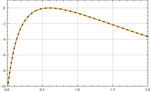
Fig. 2
Graph of from § 3 (solid line) and from (10) (dashed line) for , b = 5, and F = 4.
More generally, in a model with a scalar parameter θ generating a variance component in the form , the likelihood equation for θ is
at , where and, by the Woodbury identity,
The second derivative of at an arbitrary point is
where . A general analytic approximation to the curvature has not been ascertained. However, if is of the form θV with V a known matrix, then and the previous display simplifies. In particular,
and
so that . By consistency of the maximum likelihood estimator, the marginal loglikelihood function has zero curvature at the maximising point when the true value of θ is arbitrarily large.
6 Numerical illustrations
6.1 Covariance determined by split-plot nested blocking
The split-plot covariance is a linear combination of the identity and a binary matrix such that Vij = 1 if observational units i, j belong to the same whole plot or block. Chapter 1 of McCullagh (2023) discusses an example of this type with l = 24 rats constituting the blocks, and s = 5 sites on each rat constituting the observational units. A two-level treatment was assigned at random to the rats, so the model formula site+treat for the expected value determines a subspace of dimension 6. This is not a split-plot design in the traditional sense because the split-plot effect is associated with a classification factor, sites ranging from anterior to caudal, not with a treatment factor.
The real experiment is a little more complicated because some components are missing. With this exception, the simulated data mirror that example, and illustrate the effect of increasing θ on the discrepancy between Λ and W2. Since for the actual experiment, the range was used for simulation. For each of the 1000 Monte Carlo replications, outcomes were generated according to the model , the particular point being immaterial for the REML likelihood. As it happens, the analysis of § 3 applies here with two modified mean squares, one for treatment and one for residuals eliminating additive row and column effects, namely,
where and, for example, is the projection of Y on the subspace spanned by the treatment basis. For the null hypothesis θ = 0, Fig. 3 compares the simulated values of with the linear approximation from (2).
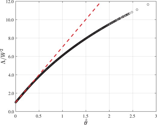
Fig. 3
Simulated plotted against for the nested-block arrangement with l = 24 large blocks and s = 5 nested blocks.
Maximization of the marginal loglikelihood function from (9) is equivalent. Both normed loglikelihood functions are graphed in Fig. 2 for , from which the anomalous geometry is apparent.
6.2 Covariance determined by Latin square blocking
The Latin square covariance is a linear combination of the identity and two binary matrices of the form if observational units i and j share a column and if they share a row. For the simulation, the variance-component parameters were taken as , while θ1 was varied in the range . The relevant mean squares on and degrees of freedom are
where . The analogous mean square for rows on f2 = f1 degrees of freedom is used in variance estimation. Specifically, the information about θ1, having adjusted for estimation of and θ2, is
In (11), θj is estimated as the positive part of with . For , which amounts to b being large, the adjustment is negligible provided that θ2 is not too large relative to θ1, and (11) is comparable to (1). The resulting Wald statistic for testing the hypothesis is to be compared with Λ, whose form is identical to that of § 3.
Figure 4 depicts qualitatively similar behaviour for the ratio as that of Fig. 3, with additional variability attributable to randomness in manifesting through the estimate of (11). The version with θ2 treated as known is depicted in Fig. 4(b).
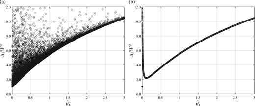
Fig. 4
Simulated plotted against for the Latin square with b = 6 rows, columns and treatments. (a): θ2 estimated in (11); (b): θ2 treated as known.
Acknowledgement
Section 3.4 was based on a detailed comparison supplied by one of the two referees, to whom we are grateful.
Supplementary material
The Supplementary Material provides more explicit derivations for some of the key results, together with a discussion of three further Wald statistics and two score statistics.
References
Bartlett
M. S
. (
1937
).
Properties of sufficiency and statistical tests
.
Proc. R. Soc. A
155
,
268
–
82
.
Chernoff
H
. (
1954
).
On the distribution of the likelihood ratio
.
Ann. Math. Statist.
25
,
573
–
8
.
Dickey
D. A.
(
2020
).
A warning about Wald tests
.
SAS Global Forum
, Paper
5088
-
2020
.
Geyer
C. J
. (
1994
).
On the asymptotics of constrained M-estimation
.
Ann. Statist.
22
,
1993
–
2010
.
Kariya
T
. (
1980
).
Locally robust tests for serial correlation in least squares regression
.
Ann. Statist.
8
,
1065
–
70
.
King
M. L.
(
1980
).
Robust tests for spherical symmetry and their application to least squares regression
.
Ann. Statist.
8
,
1265
–
71
.
McCullagh
P
. (
2009
).
Marginal likelihood for distance matrices
.
Statist. Sinica
19
,
631
–
49
.
McCullagh
P.
(
2023
).
Ten Projects in Applied Statistics
.
Cham
:
Springer
.
Patterson
H. D.
,
Thompson
R
. (
1971
).
Recovery of inter-block information when block sizes are unequal
.
Biometrika
58
,
545
–
54
.
Self
S. G.
,
Liang
K-Y
. (
1987
).
Asymptotic properties of maximum likelihood estimators and likelihood ratio tests under nonstandard conditions
.
J. Am. Statist. Assoc
.
82
,
605
–
10
.
Vu
H. T. V.
,
Zhou
S
. (
1997
).
Generalization of likelihood ratio tests under nonstandard conditions
.
Ann. Statist.
22
,
1993
–
2010
.
Wald
A
. (
1947
).
A note on regression analysis
.
Ann. Math. Statist.
18
,
586
–
9
.
© The Author(s) 2023. Published by Oxford University Press on behalf of Biometrika Trust.
This is an Open Access article distributed under the terms of the Creative Commons Attribution License (
https://creativecommons.org/licenses/by/4.0/), which permits unrestricted reuse, distribution, and reproduction in any medium, provided the original work is properly cited.


