


Summary
Nonparametric covariate adjustment is considered for log-rank-type tests of the treatment effect with right-censored time-to-event data from clinical trials applying covariate-adaptive randomization. Our proposed covariate-adjusted log-rank test has a simple explicit formula and a guaranteed efficiency gain over the unadjusted test. We also show that our proposed test achieves universal applicability in the sense that the same formula of test can be universally applied to simple randomization and all commonly used covariate-adaptive randomization schemes such as the stratified permuted block and the Pocock–Simon minimization, which is not a property enjoyed by the unadjusted log-rank test. Our method is supported by novel asymptotic theory and empirical results for Type-I error and power of tests.
1 Introduction
In clinical trials, adjusting for baseline covariates has been widely advocated as a way to improve efficiency for demonstrating treatment effects ‘under approximately the same minimal statistical assumptions that would be needed for unadjusted estimation’ (ICH E9, 1998; EMA, 2015; FDA, 2023). In testing for an effect between two treatments with right-censored time-to-event outcomes, adjusting for covariates using the Cox proportional hazards model has been demonstrated to yield valid tests even if the Cox model is misspecified (Lin & Wei, 1989; Kong & Slud, 1997; DiRienzo & Lagakos, 2002). However, these tests may be less powerful than the log-rank test that does not adjust for any covariates when the Cox model is misspecified (Kong & Slud, 1997). Although efforts have been made to improve the efficiency of the log-rank test through covariate adjustment from semiparametric theory (Lu & Tsiatis, 2008; Moore & van der Laan, 2009), the solutions are complicated and their validity is established only under simple randomization, i.e., treatments are assigned to patients completely at random.
To balance the number of patients in each treatment arm across baseline prognostic factors in clinical trials with sequentially arrived patients, covariate-adaptive randomization has become the new norm. From 1989 to 2008, covariate-adaptive randomization was used in more than 500 clinical trials (Taves, 2010); among nearly 300 trials published in two years, 2009 and 2014, 237 of them applied covariate-adaptive randomization (Ciolino et al., 2019). The two most popular covariate-adaptive randomization schemes are the stratified permuted block (Zelen, 1974) and the Pocock–Simon minimization (Taves, 1974; Pocock & Simon, 1975). Other schemes can be found in the reviews of Schulz & Grimes (2002) and Shao (2021). Unlike simple randomization, covariate-adaptive randomization generates a dependent sequence of treatment assignments, which may render conventional methods developed under simple randomization not necessarily valid under covariate-adaptive randomization (EMA, 2015; FDA, 2023). For time-to-event data under covariate-adaptive randomization, Ye & Shao (2020) showed that some conventional tests including the log-rank test are conservative and Wang et al. (2023) showed that the Kaplan–Meier estimator of the survival function has reduced variance compared to that under simple randomization.
The discussion so far has brought up two issues in adjusting for covariates. First is the need for guaranteed efficiency gains over unadjusted methods, without requiring additional assumptions. Second is the need for methods with wide applicability to all commonly used covariate-adaptive randomizations. These issues have been well addressed when adjustments are made under linear working models for non-time-to-event data (Tsiatis et al., 2008; Zhang et al., 2008; Lin, 2013; Ye et al., 2022). Ye et al. (2022) also showed that adjustment via linear working models can achieve universal applicability in the sense that the same inference procedure can be universally applied to all commonly used covariate-adaptive randomization schemes, a desirable property for application. For right-censored time-to-event outcomes, to the best of our knowledge, no result has been established for covariate adjustment with guaranteed efficiency gain and universal applicability.
In this paper we propose a nonparametric covariate adjustment method for the log-rank test, which has a simple explicit form and can achieve the goal of guaranteed efficiency gain over the unadjusted log-rank test as well as universal applicability to simple randomization and all commonly used covariate-adaptive randomization schemes. The unadjusted log-rank test is not valid under covariate-adaptive randomization; although it can be modified to be applicable to some randomization schemes (Ye & Shao, 2020), the modification needs to be tailored to each randomization scheme, i.e., no universal applicability. Our main idea is to obtain a particular derived outcome for each patient from linearizing the log-rank test statistic and then apply the generalized regression adjustment or augmentation (Cassel et al., 1976; Lu & Tsiatis, 2008; Tsiatis et al., 2008; Zhang et al., 2008) to the derived outcomes. We also develop parallel results for the stratified log-rank test with adjustment for additional covariates. Our proposed tests are supported by novel asymptotic theory of the existing and proposed statistics under the null hypothesis and alternative without requiring any specific model assumption, and under all commonly used covariate-adaptive randomization schemes. Estimation and confidence intervals for treatment effects after testing are also discussed. Our theoretical results are corroborated by a simulation study that examines finite sample Type-I error and power of tests. A real data example is included for illustration.
2 Preliminaries
For a patient from the population under investigation, let Tj and Cj be the potential failure time and right-censoring time, respectively, under treatment j = 0 or 1, and W be a vector containing all observed baseline covariates. Suppose that a random sample of n patients is obtained from the population with independent , identically distributed as . For each patient, only one of the two treatments is received. Thus, if patient i receives treatment j, then the observed outcome with possible right censoring is , where δij is the indicator of the event .
Let Ii be a binary treatment indicator for patient i and be the prespecified treatment assignment proportion for treatment 1. Consider the design, i.e., the generation of the Ii for n sequentially arrived patients. Simple randomization assigns patients to treatments completely at random with for all i, which does not make use of baseline covariates and may yield treatment proportions that substantially deviate from the target π across levels of some prognostic factors. Because of this, covariate-adaptive randomization using a subvector Z of W is widely applied, which does not use any model and is nonparametric. All commonly used covariate-adaptive randomization schemes satisfy the following mild condition (Baldi Antognini & Zagoraiou, 2015).
The covariate Z for which we want to balance in treatment assignment is an observed discrete baseline covariate with finitely many joint levels; conditioned on is conditionally independent of ; for all i and, for every level z of Z, in probability as , where nz is the number of patients with Zi = z and is the number of patients with Zi = z and Ii = 1.
Although simple randomization is not counted as covariate-adaptive randomization, it also satisfies Condition 1.
We focus on testing the following null hypothesis of the no-treatment effect, which is the null hypothesis when the conventional log-rank test is applied: for all times t, versus the alternative that H 0 does not hold, where is the unspecified hazard function of Tj, unconditional on covariates.
After data are collected from all patients, a test statistic is a function of observed data, constructed such that H 0 is rejected if and only if , where α is a given significance level and is the th quantile of the standard normal distribution. A test is asymptotically valid if, under H 0, , with equality holding for at least one parameter value under the null hypothesis H 0. A test is asymptotically conservative if, under H 0, there exists an α 0 such that .
The log-rank test in (1) is valid under simple randomization and the following assumption.
We have , where I is the treatment indicator, denotes independence and the vertical line denotes conditioning.
Assumption 1 is needed for a valid nonparametric log-rank test without requiring any model on Tj or Cj (Kong & Slud, 1997; DiRienzo & Lagakos, 2002; Lu & Tsiatis, 2008; Parast et al., 2014; Zhang, 2015).
As does not utilize any baseline covariate information, it is used as the benchmark in considering baseline covariate adjustment for efficiency gain, under the same Assumption 1 ‘that would be needed for unadjusted’ (FDA, 2023).
There is a line of research weakening Assumption 1 to censoring at random (Robins & Finkelstein, 2000; Lu & Tsiatis, 2011; Díaz et al., 2019), under which, however, the log-rank test is not valid and needs to be replaced by a weighted log-rank test that requires a correctly specified censoring distribution as the weights are inverse probabilities of censoring. Thus, the conditions and properties of weighted log-rank tests are not comparable with those of the log-rank test. Furthermore, the validity of weighted log-rank tests has only been established under simple randomization. The study of weighted log-rank tests under covariate-adaptive randomization is left for future work.
3 Covariate-adjusted log-rank test
Let be the vector containing observed baseline covariates to be adjusted in the construction of tests, with a nonsingular covariance matrix . In this section, we develop a nonparametric covariate-adjusted log-rank test that has a simple and explicit formula, enjoys guaranteed efficiency gain over the log-rank test and is universally valid under all covariate-adaptive randomization schemes satisfying Condition 1.
Asymptotic properties of covariate-adjusted log-rank test in (6) are established in the following theorem. All technical proofs are given in the Supplementary Material. In what follows, and , respectively, denote convergence in distribution and in probability, as .
Suppose that Condition 1 and Assumption 1 hold, and that all levels of Zi used in covariate-adaptive randomization are included in Xi as a subvector. Then, the following results hold regardless of which covariate-adaptive randomization scheme is applied.
- Under the null H0 or alternative hypothesis,
where , nj is the number of patients in treatment j, and .
- Under the null hypothesis H0,
i.e., is valid.
- Under the local alternative hypothesis that with the cj not depending on n and that is bounded and tends to 1 for every t,
The results under an alternative hypothesis in Theorem 1 are obtained without any specific model on the distribution of Tj or Cj, different from many published research articles that assume a specific model under an alternative hypothesis, such as the Cox proportional hazards model for Tj.
Theorem 1 shows that in (6) is applicable to all randomization schemes satisfying Condition 1 with a universal formula, if all levels of Zi are included in Xi. Tests with universal applicability are desirable for application, as the complication of using tailored formulas for different randomization schemes is avoided.
To show that in (6) has a guaranteed efficiency gain over the benchmark in (1), we establish an asymptotic result for under covariate-adaptive randomization satisfying an additional condition.
. As , where is the set containing all levels of Z, Ω is the diagonal matrix whose diagonal entries are , and is a known constant depending on the randomization scheme.
Suppose that Conditions 1 and 1 and Assumption 1 hold. Then the following results hold.
- Under the null H0 or alternative hypothesis,
where nj and θj are given in Theorem 1, for ν given in Condition 1 and is defined in Theorem 1.
- Under the null hypothesis H0,
Hence, is conservative unless or almost surely under H0.
- Under the local alternative hypothesis in Theorem 1(c),
Under simple randomization, Condition 1 holds with and, hence, Theorem 2 also applies with . Under the local alternative specified in Theorem 1(c) with , by Theorems 1(c) and 2(c), Pitman’s asymptotic relative efficiency of in (6) with respect to the benchmark in (1) is with the strict inequality holding unless . Thus, has a guaranteed efficiency gain over under simple randomization.
The Pocock–Simon minimization satisfies Condition 1, but not necessarily Condition 1 as the Ii are correlated across strata. Hence, under the Pocock–Simon minimization, Theorem 2 is not applicable and may not be valid, whereas is valid according to Theorem 1, another advantage of covariate adjustment.
In the numerator of (6) is the same as the augmented score in Lu & Tsiatis (2008), which shares the same idea as those in Tsiatis et al. (2008) and Zhang et al. (2008) for noncensored data. However, the denominator in (6) is different from that used by Lu & Tsiatis (2008). The key difference between our result on guaranteed efficiency gain and the result in Lu & Tsiatis (2008) is that our result is obtained under covariate-adaptive randomization and an alternative hypothesis without any specific model on the distribution of Tj or Cj, whereas the result in Lu & Tsiatis (2008) is for simple randomization and an alternative hypothesis under a correctly specified Cox proportional hazards model for Tj.
After testing H 0, it is often of interest to estimate and construct a confidence interval for an effect size (Lu & Tsiatis, 2008; Parast et al., 2014; Zhang, 2015; Díaz et al., 2019). A commonly considered effect size is the hazard ratio under the Cox proportional hazards model . The hazard ratio is interpretable only when the Cox proportional hazards model is correctly specified. Thus, in the rest of this section we consider covariate-adjusted estimation and a confidence interval for θ, assuming that .
4 Covariate-adjusted stratified log-rank test
The stratified log-rank test (Peto et al., 1976) is a weighted average of the stratum-specific log-rank test statistics with finitely many strata constructed using a discrete baseline covariate. We consider stratification with all levels of Zi. Results can be obtained similarly for stratifying on more levels than those of Zi or fewer levels than those of Zi with levels of Zi not used in stratification included in Xi. Here, we remove the part of Xi that can be linearly represented by Zi and still denote the remaining as Xi. As such, it is reasonable to assume that is positive definite.
and .
With stratification, in (7) actually tests the null hypothesis for all (t, z), where is the hazard function of Tj conditional on Z = z. Hypothesis may be stronger than for all t, the null hypothesis for unstratified log-rank test and its adjustment considered in § 2–§ 3. In some scenarios, . For example, the two hypotheses are the same when there exists a transformation model for all (t, W) and an unknown constant θ, where h is an increasing function that is possibly unknown (Cheng et al., 1995). This transformation model includes many commonly used semiparametric models as special cases, for example the Cox proportional hazards model with .
The following theorem establishes the asymptotic properties of the stratified log-rank test and covariate-adjusted stratified log-rank test .
Suppose that Condition 1 holds and that . Then, the following results hold regardless of which covariate-adaptive randomization is applied.
- Under the null or alternative hypothesis,
and the same result holds with and replaced by and , respectively, where , nzj is the number of patients with treatment j in stratum z, j = 0, 1, and .
- Under the null hypothesis ,
i.e., both and are valid for testing null hypothesis .
- Under the local alternative hypothesis that with the czj not depending on n and that is bounded and tends to 1 for every t and z,
and the same result holds with and replaced by and , respectively.
Like in (6), both in (7) and in (8) are applicable to all covariate-adaptive randomization schemes with universal formulas, i.e., they achieve the universal applicability. In terms of Pitman’s asymptotic efficiency under the local alternative specified in Theorem 3(c), is always more efficient than , since with the strict inequality holding unless .
The condition in Theorem 3 for the stratified log-rank test and its adjustment is in general not comparable with Theorem 1(c) for the unstratified log-rank test.
Is or more efficient than the unstratified log-rank test ? The answer is not clear because, firstly, the null hypotheses and H 0 may be different, as we discussed earlier, and secondly, even if , under the alternative, the asymptotic mean of may not be comparable with the asymptotic mean of or . In fact, the indefiniteness of relative efficiency between the stratified and unstratified log-rank tests is a standing problem in the literature.
There is also no definite answer when comparing the efficiencies of and the stratified .
Similar to the discussion at the end of § 3, after testing hypothesis , we can obtain a covariate-adjusted confidence interval for the effect size θ under a stratified Cox proportional hazards model for every z; see the Supplementary Material for further details.
5 Simulations
To supplement the theory and examine finite sample Type-I error and power of tests and , we carry out a simulation study under the following four cases/models.
The conditional hazard function follows a Cox model, for j = 0, 1, where θ denotes a scalar parameter, and W is a three-dimensional covariate vector following the three-dimensional standard normal distribution. The censoring variables C 0 and C 1 follow a uniform distribution on the interval (10, 40) and are independent of W.
The conditional hazard function is the same as that in Case I. Conditional on W and treatment assignment j, follows a standard exponential distribution.
We have , where θ, η and W are the same as in Case I, and is a random variable independent of and has the standard exponential distribution. The setting for censoring is the same as that in Case I.
The models for the Tj and Cj are the same as those in Cases III and II, respectively.
In this simulation, the significance level , the target treatment assignment proportion , the overall sample size n = 500, the null hypothesis , and since a transformation model described in § 4 holds in Cases I–IV. Three randomization schemes are considered: simple randomization, stratified permuted block randomization with block size 4 and levels of Z as strata, and the Pocock–Simon minimization assigning a patient with probability 0.8 to the preferred arm minimizing the sum of balance scores over marginal levels of Z, where Z is the two-dimensional vector whose first component is a two-level discretized first component of W and the second component is a three-level discretized second component of W. For stratified log-rank tests, levels of Z are used as strata. For covariate adjustment, X is the vector containing Z and the third component of W for , and X is the third component of W for .
Based on 10 000 simulations, Type-I error rates for four tests under four cases and three randomization schemes are shown in Table 1. The results agree with our theory. For and , there is no substantial difference among the three randomization schemes. The log-rank test preserves the 5% rate under simple randomization, but it is conservative under stratified permuted block randomization and minimization.
Type-I errors (in percentages) based on 10 000 simulations
| Case | Randomization | ||||
|---|---|---|---|---|---|
| I | Simple | 4.91 | 5.16 | 4.86 | 4.78 |
| Permuted block | 3.25 | 5.22 | 4.80 | 4.85 | |
| Minimization | 3.40 | 5.43 | 5.02 | 5.23 | |
| II | Simple | 5.39 | 5.14 | 5.00 | 4.97 |
| Permuted block | 3.59 | 5.03 | 4.94 | 4.82 | |
| Minimization | 4.01 | 5.23 | 5.11 | 5.28 | |
| III | Simple | 5.07 | 5.43 | 5.27 | 5.16 |
| Permuted block | 2.29 | 4.79 | 4.76 | 4.82 | |
| Minimization | 2.88 | 5.43 | 5.23 | 5.52 | |
| IV | Simple | 5.41 | 5.30 | 5.39 | 5.21 |
| Permuted block | 4.44 | 5.48 | 5.10 | 5.49 | |
| Minimization | 4.21 | 5.18 | 5.04 | 5.06 |
Based on 10 000 simulations, power curves of four tests for θ ranging from 0 to 0.6, under four cases and stratified permuted block randomization are plotted in Fig. 1. Similar figures for simple randomization and minimization are given in the Supplementary Material. In all cases, the power curves of covariate-adjusted tests and are better than those of unadjusted tests and , especially the benchmark . Under Cox’s model, is better than , but not necessarily under the non-Cox model. The stratified is mostly better than the unstratified , but unlike and , there is no guaranteed efficiency gain, e.g., case III when . The difference in censoring model also has some effect.
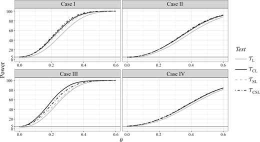
Power curves based on 10 000 simulations.
More simulation results can be found in the Supplementary Material.
6 A real data application
We apply four tests and to the data from the AIDS Clinical Trials Group Study 175, ACTG 175, a randomized controlled trial evaluating antiretroviral treatments in adults infected with human immunodeficiency virus type 1 whose CD4 cell counts were from 200 to 500 per cubic millimeter (Hammer et al., 1996). The primary endpoint was time to a composite event defined as a % decline in the CD4 cell count, an AIDS-defining event, or death. Stratified permuted block randomization with equal allocation was applied with covariate Z having three levels related with the length of prior antiretroviral therapy: Z = 1, 2 and 3, representing 0 weeks, between 1 to 52 weeks and more than 52 weeks of prior antiretroviral therapy, respectively. The dataset is publicly available in the R package speff2trial (R Development Core Team, 2024).
We focus on the comparison of treatment 0 (zidovudine) versus treatment 1 (didanosine). For stratified log-rank test , the three-level Z is used as the stratification variable. For covariate adjustment, two additional prognostic baseline covariates are considered as X: the baseline CD4 cell count and the number of days receiving antiretroviral therapy prior to treatment. In addition to testing treatment effect for all patients, a subgroup analysis with Z strata as subgroups is also of interest because responses to antiretroviral therapy may vary according to the extent of prior drug exposure. Within each subgroup defined by Z, the stratified tests become the same as their unstratified counterparts, and thus we only apply tests and in the subgroup analysis.
Table 2 reports the number of patients, numerator and denominator of each test, and a p-value for testing with all patients or with a subgroup. The effect of covariate adjustment is clear: for the covariate-adjusted tests, the standard errors and are smaller than and in all analyses.
Statistics for the ACTG 175 example
| Subgroup | ||||
|---|---|---|---|---|
| All patients | Z = 1 | Z = 2 | Z = 3 | |
| Number of patients | 1093 | 461 | 198 | 434 |
| Log-rank test | ||||
| –1.223 | –0.542 | –0.144 | –1.292 | |
| 0.265 | 0.235 | 0.270 | 0.290 | |
| p-value (adjusted for subgroup analysis) | < 0.001 | 0.064 | 1 | < 0.001 |
| Estimated θ | –0.528 | –0.455 | –0.140 | –0.740 |
| Standard error of the estimated θ | 0.116 | 0.199 | 0.263 | 0.171 |
| Covariate-adjusted log-rank test | ||||
| –1.273 | –0.553 | –0.129 | ||
| 0.257 | 0.230 | 0.265 | 0.282 | |
| p-value (adjusted for subgroup analysis) | < 0.001 | 0.049 | 1 | < 0.001 |
| Estimated θ | –0.550 | –0.464 | –0.127 | |
| Standard error of the estimated θ | 0.113 | 0.195 | 0.257 | 0.166 |
| Stratified log-rank test | ||||
| –1.228 | ||||
| 0.264 | ||||
| p-value | < 0.001 | |||
| Estimated θ | –0.531 | |||
| Standard error of the estimated θ | 0.116 | |||
| Covariate-adjusted stratified log-rank test | ||||
| 0.258 | ||||
| p-value | < 0.001 | |||
| Estimated θ | ||||
| Standard error of the estimated θ | 0.113 | |||
Here θ denotes the log hazard ratio for all patients and for each subgroup.
For the analysis based on all patients, all four tests significantly reject the null hypothesis H 0 of the no-treatment effect. In the subgroup analysis, the p-values are adjusted using Bonferroni’s correction to control for the familywise error rate. From Table 2, p-values in the subgroup analysis are substantially larger than those in the analysis of all patients, because of reduced sample sizes as well as Bonferroni’s correction. The empirical result in this example illustrates the benefit of covariate adjustment in testing when the sample size is not very large. Using the adjusted log-rank test , together with the estimated effect size and its standard error shown in Table 2, we can conclude the superiority of treatment 1 for both Z = 1 and Z = 3, which is consistent with the evidence of Hammer et al. (1996).
Acknowledgement
We would like to thank all reviewers for useful comments and suggestions. Our research was supported by the National Natural Science Foundation of China and the U.S. National Science Foundation. Shao is also affiliated with the East China Normal University.
Supplementary material
The Supplementary Material contains all technical proofs and some additional results.
References
