


Abstract
The degeneration of flight ability has contributed to the diversification of beetles, which are among the most diverse groups in the world. Over the course of flight ability degeneration, intraspecific polymorphisms in flight traits occur. The type of habitat in which degeneration of flight ability is likely to occur is an important issue for understanding the diversification process of beetles, but this topic has rarely been studied in detail. In this study, we examined two closely related species (one species with intraspecific polymorphisms in the hind wings and the other an apterous-monomorphic species) of the genus Synuchus to clarify this issue. Our study indicated that these two species were morphologically and genetically related, but they showed contrasting genetic differentiation patterns and inhabited different environmental conditions. In particular, the apterous-monomorphic species seemed to be isolated in mountainous environments with four major climatic and terrain characteristics (cool, heavy precipitation in winter, large temperature and precipitation differences, and low continuity among habitats), and this isolation might have contributed to their complete loss of flight ability and geographical genetic differentiation via further suppression of gene flows between populations.
INTRODUCTION
Insects are one of the most diversified groups on the Earth (Grimaldi and Engel 2005), estimated to include ~5.5 million species (including undescribed species) (Stork 2018). Acquisition of the ability to fly has enabled insects to disperse to new habitats and has contributed to the current prosperity of insects (Roff and Fairbairn 1991, Whiting et al. 2003). In contrast, secondary degeneration of hind wings has occurred in multiple lineages of winged insects, and ~10% of all insects are estimated to be flightless (Roff 1990). In addition, winged insects are occasionally flightless owing to the loss of flight muscles (Ikeda et al. 2012). Degeneration of flight ability in insects could contribute to genetic differentiation among populations through a decrease in dispersal opportunities (Peterson and Denno 1998), which results in the diversification of insects. In insects, degeneration of flight ability occurs in the following order: reduction of flight frequency, degeneration of flight muscles, then degeneration of wings (Roff 1986). In each degeneration stage, intraspecific polymorphisms in morphological traits related to flight ability (flight traits) can be observed (Den Boer et al. 1980, Harrison 1980). Thus, intraspecific polymorphisms in flight traits indicate that flight ability is undergoing degeneration in the species. Analysing the relationship between polymorphisms in flight traits and genetic differentiation among populations would contribute to clarifying the impact of the degeneration of flight ability on insect diversification.
The order Coleoptera is the most diverse group of insects, accounting for ~40% of insect species diversity (Cai et al. 2022). Degeneration of flight ability might be one of the major drivers of vast diversification in beetles (Ikeda et al. 2012, Sota et al. 2022). Ground-dwelling beetles include many flightless and flight polymorphic species (Lövei and Sunderland 1996). Regarding ground-dwelling beetles, it is known that the proportion of flightless individuals increases in habitats with high homogeneity (Den Boer et al. 1980), and degeneration of flight ability tends to occur in geographically isolated environments, such as islands or mountains (Darlington 1943, Sota et al. 2020). In general, investment in the ability to fly allows ground-dwelling beetles to disperse from inappropriate habitats to suitable ones; however, it is also costly for them (Darlington 1943, Roff 1986). Therefore, if they have achieved dispersal into suitable habitats with homogeneity and/or isolation, they might no longer need to maintain high dispersal ability, and the degeneration of flight ability might happen. Thus, factors related to the environment, such as environmental heterogeneity and geographical variables, as proposed by Roff (1990), seem to be major contributors to the decrease in the flight ability of ground-dwelling beetles. In addition, gene flow can be interrupted within isolated habitat environments with high heterogeneity (Liebherr 1988), and genetic differentiation is expected to be promoted in such environments. Indeed, climatic and geographical factors in habitats affect the geographical patterns of flight trait polymorphism and dispersal ability in ground-dwelling beetles, resulting in genetic differentiation among populations (e.g. Ohta et al. 2009, Ikeda and Sota 2011). Such studies are also important for revealing factors responsible for the degeneration of flight ability and processes leading to speciation in beetles.
The genus Synuchus Gyllenhal, 1810, is a group of ground-dwelling beetles belonging to the family Carabidae, and 38 species inhabit the Japanese archipelago (Mori 2015, Morita 2022). Recently, polymorphisms in flight traits have been found in several species in this genus (e.g. Hori 2008, Shibuya et al. 2018, Shimizu et al. 2024). Synuchus arcuaticollis (Motschulsky, 1860) is one of the most common Synuchus species in the Japanese archipelago (Tanaka 1985) and retains polymorphisms in its hind wings (Habu 1955, Tanaka 1962, Shibuya et al. 2018, Shimizu et al. 2024). In S. arcuaticollis, most individuals are macropterous, but brachypterous individuals also emerge at a rate of ~10%, and apterous individuals occur rarely (Shimizu et al. 2024). Therefore, S. arcuaticollis might be experiencing ongoing degeneration of its ability to fly. In addition, a species that is morphologically similar to S. arcuaticollis but is apterous-monomorphic was found in a mountainous area in Honshu, Japan (Synuchus sp. 2 in the study by Shimizu et al. 2024). This species could be a cryptic species closely related to S. arcuaticollis, consisting of the S. arcuaticollis species complex (see ‘Results of phylogenetic analysis’ and ‘Taxonomic notes’ in the Supporting Information). Thus, the S. arcuaticollis species complex is suitable for examining the relationships among flight traits, genetic differentiation, and the environment.
Our purpose in this study was to clarify whether and how interspecific differences in habitat environments lead to interspecific differences in flight trait degeneration and genetic differentiation in the S. arcuaticollis species complex. In particular, we examined the flight traits of individuals collected across the distributional ranges, estimated genetic differentiation and demographic processes via a series of DNA sequence analyses, and evaluated their habitat environments, distribution probabilities, and habitat discontinuity based on distribution records. Finally, we discussed the contribution of the environment to the degeneration of flight traits and genetic differentiation.
MATERIALS AND METHODS
Sample collection and species identification
We collected 118 individuals of the S. arcuaticollis species complex from 49 sites throughout the Japanese archipelago (Hokkaido, Honshu, Shikoku, Kyushu, Oki Islands, and Tsushima; Fig. 1; Supporting Information Tables S1 and S2). Pitfall traps and night searching methods were used to collect samples. In this study, one of the species matching Habu’s (1978) morphological description of S. arcuaticollis was defined as ‘Synuchus sp. A’ (equivalent to S. arcuaticollis in paper by Shimizu et al. 2024). We defined the other species as ‘Synuchus sp. B’ (equivalent to Synuchus sp. 2 in the paper by Shimizu et al. 2024), because we could not determine which species was the ‘true’ S. arcuaticollis (see ‘Taxonomic notes’ in the Supporting Information).
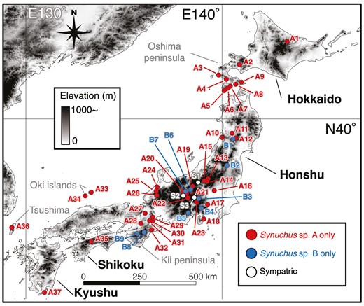
Map of sampling sites in the Japanese archipelago. Dots indicate the occurrence points, and colours correspond to the collected species. The numbers correspond to the site numbers in Supporting Information, Table S1. This map was created by QGIS.
We selected two species (Dolichus halensis and Pristosia aeneola) as the outgroup for phylogenetic analysis and collected one individual from each species. The selection of the outgroup was based on a previous phylogenetic study of the tribe Sphodrini (including the genus Synuchus) by Ruiz et al. (2009). Furthermore, we selected three species (Synuchus nitidus, Synuchus cycloderus, and Synuchus melantho) within the genus Synuchus as the outgroup for phylogenetic analysis according to Kudo et al. (2019) and used one individual per species.
In total, 123 individuals of five species were used for the study. All the samples were preserved in 99.5% ethanol and stored at room temperature or −30°C.
Analysis of flight traits
We dissected all the individuals of the S. arcuaticollis species complex to analyse traits related to flight ability (flight traits). In this study, we focused on flight muscles and hind wings for flight traits because these morphological traits are directly linked to the flight ability of carabid beetles (Matalin 2003). Dissection was conducted with a binocular stereomicroscope or an optical microscope, and the conditions of the flight muscles and hind wings were observed. The flight muscles were classified as either present or absent. The hind wings were classified into three types: macropterous (with well-developed veins and an oblongum); brachypterous (with faint veins and without a distinct oblongum); and apterous (without hind wings) (Supporting Information, Fig. S1).
In addition, to clarify the relationship between hind wing degeneration and genotype, the states of the hind wings and mitochondrial haplotype in each individual were checked and shown in the Bayesian phylogenetic tree constructed by partial sequences of mitochondrial DNA (see ‘Phylogenetic analysis and divergence time estimation’).
DNA extraction, amplification, sequencing, and alignment
Total genomic DNA was extracted from the muscle tissue of the hind legs or metathorax of 123 individuals via a Wizard Genomic DNA Purification Kit (Promega, Madison, WI, USA). We conducted PCR and amplified partial sequences of mitochondrial DNA (mtDNA) and nuclear DNA (nuDNA) with a Gene Amp PCR System 9700 (Thermo Fisher Scientific, Waltham, MA, USA) or VeritiPro Thermal Cycler (Thermo Fisher Scientific). One mitochondrial gene, cytochrome c oxidase subunit I (COI), and one nuclear gene, 28S rDNA (28S), were amplified and sequenced. We used C1-J-2183 (5ʹ-CAACATTTATTTTGATTTTTTGG-3ʹ) and L2-N-3014 (5ʹ-TCCAATGCACTAATCTGCCATATTA-3ʹ) as mtDNA COI primers (Simon et al. 1994). We also used 28S-D1 (5ʹ-GGGAGGAAAAGAAACTAAC-3ʹ) and 28S-D3 (5ʹ-GCATAGTTCACCATCTTTC-3ʹ) as nuDNA 28S primers (Sasakawa and Kubota 2007). The PCR protocol for COI and 28S was 94°C for 3 min; 30 × (94°C for 1 min, 48°C or 50°C for 1 min, and 72°C for 1 min); and 72°C for 7 min. The PCR products were purified with an Illustra ExoStar Clean-Up Kit (GE Healthcare, Chicago, IL, USA). The purified PCR products were sequenced using sequencing services provided by Macrogen Japan (Koto, Tokyo, Japan) or Fasmac (Atsugi, Kanagawa, Japan). All sequence data were checked using MEGA7 (Kumar et al. 2016), and obvious sequencing errors were corrected. COI sequences were aligned by ClustalW (Thompson et al. 2002) implemented in MEGA7, and 28S sequences were aligned by the L-INS-I method implemented in MAFFT v.7 (Katoh et al. 2019). All sequence data were deposited in the DNA Data Bank of Japan (DDBJ; accession numbers are shown in Supporting Information, Table S3).
Phylogenetic analysis and divergence time estimation
We conducted phylogenetic analysis and divergence time estimation based on the COI region and 28S region by the Bayesian and maximum likelihood (ML) methods using 123 individuals of five species. Before phylogenetic analysis and divergence time estimation, we removed the duplicated haplotypes for each region via DnaSP v.5 (Librado and Rozas 2009) and selected the nucleotide substitution models using Kakusan4 (Tanabe 2011) and ModelTest-NG (Darriba et al. 2020) for the Bayesian and ML method, respectively. We used the Bayesian information criterion (BIC; Schwarz 1978) calculated from the alignment length (BIC4 in Kakusan4) and used the corrected Akaike’s information criterion based on the Akaike’s information criterion (Akaike 1974) for the Bayesian and ML method, respectively. In the model selection procedure, we compared proportional and separate models by codon position in the protein-coding region (i.e. COI region) and did not consider them in the non-coding region (i.e. 28S region).
We used MrBayes v.3.2.6 (Ronquist et al. 2012) to construct Bayesian inference (BI) phylogenetic trees. The codon proportional model was selected for the COI region (first codon, HKY+Gamma; second codon, HKY+Gamma; and third codon, GTR+Gamma), and HKY+Gamma was selected for the 28S region. To construct the COI tree, Markov chain Monte Carlo (MCMC) chains were run for 10 000 000 generations, with trees sampled every 1000 generations. To construct the 28S tree, MCMC chains were run for 1 000 000 generations, with trees sampled every 100 generations. The burn-in rate was set to 25% for both analyses. After all the analyses were completed, we confirmed the convergence of all parameters (effective sample size; ESS > 200) by using Tracer v.1.7.1 (Rambaut et al. 2018) and constructed consensus BI phylogenetic trees. Bayesian posterior probabilities were calculated and used to evaluate the clade credibility.
We used RAxML-NG (Kozlov et al. 2019) to construct ML phylogenetic trees. GTR+I+G4, TIM3+I+G4, and GTR+G4 were selected for the first, second, and third codons of the COI region, respectively, and TVM+G4 was selected for the 28S region. After constructing ML phylogenetic trees for both regions, bootstrap values were calculated and used to evaluate the branch support (1000 replications).
We used BEAST v.1.10.4 (Suchard et al. 2018) to estimate the divergence time of the S. arcuaticollis species complex via the Bayesian method. We used 120 individuals for which at least the COI region was sequenced. The codon proportional model was selected for the COI region (first codon, HKY+Gamma; second codon, HKY+Gamma; and third codon, GTR+Gamma), and HKY+Gamma was selected for the 28S region. A log-normal relaxed clock (Drummond et al. 2006) was assumed for all codons and regions. The default setting was used for the tree prior (constant size; Kingman 1982). We also set the prior distribution of the clock rate as a continuous-time Markov chain rate reference in both the COI and 28S regions. To calibrate and calculate the divergence times, we set the node where S. cycloderus and other Synuchus species diverged to 24.4 ± 4.38 Mya (mean ± SD) according to the divergence time estimation by Ruiz et al. (2009). The MCMC chains were run for 500 000 000 generations, with trees sampled every 50 000 generations. After the phylogenetic analysis was completed, we confirmed the convergence of all parameters (ESS > 200) by Tracer and constructed a consensus BI phylogenetic tree by LogCombiner v.1.10.4 and TreeAnnotator v.1.10.4 with 25% burn-in. FigTree v.1.4.4 (Rambaut 2012) was used to visualize and edit the phylogenetic trees.
Genetic diversity and geographical differentiation
We compared the genetic structures of two species in the S. arcuaticollis species complex. The COI region was used in this analysis because it showed intraspecific genetic diversity in both species (see Results). Two indices of genetic diversity (haplotype diversity and nucleotide diversity) were calculated for each species by DnaSP. Intraspecific pairwise genetic distances (p-distances) for each species and interspecific p-distances were calculated by MEGA7.
We also examined the isolation by distance for each species. Geographical distances (in kilometres) among sites were calculated by the ‘geosphere’ package (Hijmans 2022) in R v.4.3.1 (R Core Team 2013) and were log10-transformed. The p-distances among sites were calculated by MEGA7. Isolation by distance was evaluated by Pearson’s correlation coefficient and the linear regression slope, and tested based on Mantel permutation with 10 000 replications by the ‘vegan’ package (Oksanen et al. 2022) and ‘lm’ function in R.
Demographic analysis
We compared population demographies between the two species in the S. arcuaticollis species complex. The COI region was also used in this analysis. Two indices for population demography (Tajima’s D and Fu’s Fs; Tajima 1989, Fu 1997) were calculated for each species by ARLEQUIN v.3.5. (Excoffier and Lischer 2010) with 1000 replications.
To compare demographic histories between species, we performed Bayesian skyline plot analysis (Drummond et al. 2005) with BEAST. For the same reason mentioned above, we used the COI region in this analysis. The codon proportional model was selected for Synuchus sp. A (first codon, HKY+Gamma; second codon, F81+Homogeneous; and third codon, HKY+Gamma) and for Synuchus sp. B (first codon, F81+Homogeneous; second codon, F81+Homogeneous; and third codon, HKY+Gamma). A strict clock was assumed for all codons. In this analysis, we used the clock rates estimated in divergence time estimation analysis (first codon, 0.00165 ± 0.00453; second codon, 0.00190 ± 0.00185; and third codon, 0.01600 ± 0.05050) with a normal distribution. The MCMC chains were run for 50 000 000 generations, with trees sampled every 5000 generations for each species. After the analyses were completed, we confirmed the convergence of all parameters (ESS > 200) and constructed a Bayesian skyline plot with 25% burn-in by Tracer.
Distribution patterns and differences in the habitat environment
We compared the distribution patterns and habitat environments of the two species in the S. arcuaticollis species complex. Here, all 49 sites in which species were confirmed to occur were classified into two groups: sites inhabited by Synuchus sp. A and those inhabited by Synuchus sp. B (37 and 9 sites, respectively, with 3 sympatric sites). Then, we performed species distribution modelling with Maxent v.3.4.4 (Phillips et al. 2006) and estimated the potential distribution area in the Japanese archipelago for each species. To construct the species distribution models (SDMs), we used 19 bioclimatic variables related to temperature and precipitation from WorldClim (https://www.worldclim.org) at a resolution of 30 seconds″ (~1 km mesh). Given that temperature and precipitation are reported to contribute to genetic and phenotypic divergence between closely related species of carabid beetles (e.g. Tsuchiya et al. 2012, Homburg et al. 2013, Zhang and Kubota 2021), these climatic factors are also expected to influence the genetic differentiation and polymorphisms in the hind wings of the S. arcuaticollis species complex.
Here, we obtained 19 bioclimatic values from 49 sites via the ‘raster’ package (Hijmans 2023) and the ‘sp’ package (Pebesma and Bivand 2005) in R. Strong correlations among variables can interfere with the accuracy of SDMs (Zhang and Kubota 2020); therefore, we calculated pairwise Pearson’s correlation coefficients with the ‘corrplot’ package (Wei and Simko 2021) in R and excluded one of the paired variables with |r| > 0.8. As a result, seven bioclimatic variables (BIO2, BIO4, BIO8, BIO9, BIO12, BIO15, and BIO17) were selected for analyses (Supporting Information, Table S4). We confirmed that only one occurrence point was included in each mesh. The geographical range of the SDMs was clipped to include almost the entire archipelago (30.0–45.6°N, 128.5–153.8°E). The accuracy of each model was evaluated by the receiver operating characteristic curve and area under the curve. Distribution probabilities were calculated by bootstrap values, and 10 replicate runs were conducted for each SDM. After these analyses were completed, we projected the distribution probability for each species by QGIS v.3.32 (https://qgis.org/ja/site/index.html).
To clarify the differences in the habitat environment between the two species, we focused on climate conditions and the discontinuity of each habitat. For the analysis of climate conditions, we used all the 19 bioclimatic variables. Principal component analysis (PCA) based on 19 bioclimatic variables from 49 sites was performed with the ‘prcomp’ function, and the first two axes (PC1 and PC2) were projected with the ‘ggplot2’ package (Wickham 2016) in R. We obtained PC1 and PC2 scores (Supporting Information, Table S5) for the two groups of sites inhabited by the species. The normality and homoscedasticity of the PC1 and PC2 scores were tested by the Shapiro–Wilk test and F test, respectively. The normality assumption of the PC scores was frequently violated (Synuchus sp. A: PC1, W = 0.98, P = .52; PC2, W = 0.89, P = .001; and Synuchus sp. B: PC1, W = 0.83, P = .02; PC2, W = 0.74, P = .002), whereas that of homoscedasticity was met (PC1: F = 2.41, P = .119; PC2: F = 3.06, P = .051). Therefore, differences in the climate conditions between the two species were tested by the Mann–Whitney U-test using the ‘exactRankTests’ package (Hothorn and Hornik 2022) in R.
For the analysis of habitat discontinuity, we extracted elevation data and calculated the variances in elevation within the circles with a radius of 2.5, 5.0, and 10.0 km centred on each site using QGIS (Supporting Information, Table S5). The higher and lower value of this index indicate rugged and flat topologies, respectively. Thus, this index can be used as an indicator of habitat discontinuity around the site. For the analysis of habitat discontinuity, we used elevation data from WorldClim at a resolution of 30 seconds″. The normality and homoscedasticity of the values were tested by the Shapiro–Wilk test and F test, respectively. The normality assumption of the scores was met (Synuchus sp. A: 2.5 km radius, W = 0.97, P = .33; 5.0 km radius, W = 0.96, P = .17; 10.0 km radius, W = 0.97, P = .33; and Synuchus sp. B: 2.5 km radius, W = 0.97, P = .95; 5.0 km radius, W = 0.98, P = .96; 10.0 km radius, W = 0.97, P = .90) and that of homoscedasticity was also met (2.5 km radius: F = 1.49, P = .49; 5.0 km radius: F = 1.54, P = .45; 10.0 km radius: F = 1.93, P = .24). Therefore, differences in habitat discontinuity between the two species were tested by ANOVA using R.
RESULTS
Analysis of flight traits
We collected 87 individuals of Synuchus sp. A from 40 sites and 31 individuals of Synuchus sp. B from 12 sites (Fig. 1; Supporting Information, Tables S2 and S3; Fig. S2). Among the 118 individuals of the two species dissected, no individuals had tissue clearly identifiable as flight muscles. For Synuchus sp. A, most individuals were macropterous; brachypterous individuals accounted for ~10%, and only one apterous individual was found (Supporting Information, Tables S2 and S3), indicating intraspecific polymorphism of the hind wings. In contrast, all individuals were apterous in Synuchus sp. B.
Phylogenetic analysis and divergence time estimation
In Synuchus sp. A, we identified 36 haplotypes in 85 sequenced individuals for the COI region and only one haplotype in 61 sequenced individuals for the 28S region. Likewise, in Synuchus sp. B we identified 15 haplotypes in 30 sequenced individuals for the COI region and only one haplotype in 16 sequenced individuals for the 28S region. We found only one nucleotide difference within 1029 bp of the 28S region between the two species. One haplotype of COI (Hap 4) was widely shared among 16 of 40 sites from Hokkaido to Kyushu in Synuchus sp. A (Fig. 2; Supporting Information, Table S3). In contrast, although one haplotype (Hap 49) was shared at two sites on the Kii Peninsula (i.e. Sites B8 and B9) in Synuchus sp. B, most individuals retained the haplotypes unique to each site (Fig. 2; Supporting Information, Table S3). No haplotypes of either the COI region or the 28S region were shared between the two species, even at sympatric sites. Phylogenetic analyses using both Bayesian and ML methods for the COI and 28S regions revealed that these two species formed monophyletic groups and were separated into two clades corresponding to species, except for the ML tree of the COI region (Figs 2, 3; Supporting Information, Figs S3, S4). In the clade for Synuchus sp. A, brachypterous or apterous individuals were not clustered but mixed (Fig. 2).
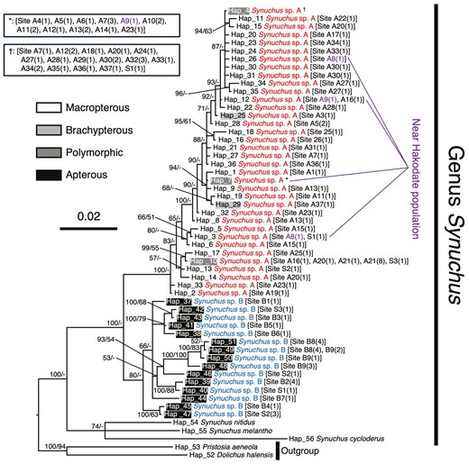
Bayesian inference (BI) phylogenetic tree of the genus Synuchus based on mitochondrial DNA COI sequences. The scale bar indicates the substitution rate (substitutions per site). The numbers next to the nodes indicate the Bayesian posterior probability (≥50%)/maximum likelihood (ML) bootstrap value (≥50%). ‘-’ indicates that the node of the BI tree did not appear in the ML tree or that the ML bootstrap value was <50%. The haplotype numbers correspond to Supporting Information, Table S3. The site numbers in square brackets correspond to Supporting Information, Table S1 and Figure 1. The numbers in parentheses indicate the numbers of individuals sharing the same haplotype. The colours of the haplotypes show the states of the hind wing in each haplotype. The purple numbers indicate the phylogenetic positions of individuals collected near Hakodate (i.e. sites A8 and A9). *,†These haplotypes are shared by many individuals, as listed in the key.
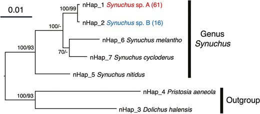
Bayesian inference (BI) phylogenetic tree of the genus Synuchus based on nuclear DNA 28S sequences. The scale bar indicates the substitution rate (substitutions per site). The numbers next to the nodes indicate the Bayesian posterior probability (≥50%)/maximum likelihood (ML) bootstrap value (≥50%). ‘-’ indicates that the node of the BI tree did not appear in the ML tree or that the ML bootstrap value was <50%. The haplotype numbers correspond to Supporting Information, Table S3. The numbers in parentheses indicate the numbers of individuals sharing the same haplotype.
Divergence time estimation revealed that Synuchus sp. A and Synuchus sp. B diverged from their most recent common ancestor at 7.18 Mya (Fig. 4). In addition, intraspecific phylogenetic divergence started earlier in Synuchus sp. B (3.73 Mya) than in Synuchus sp. A (1.77 Mya).
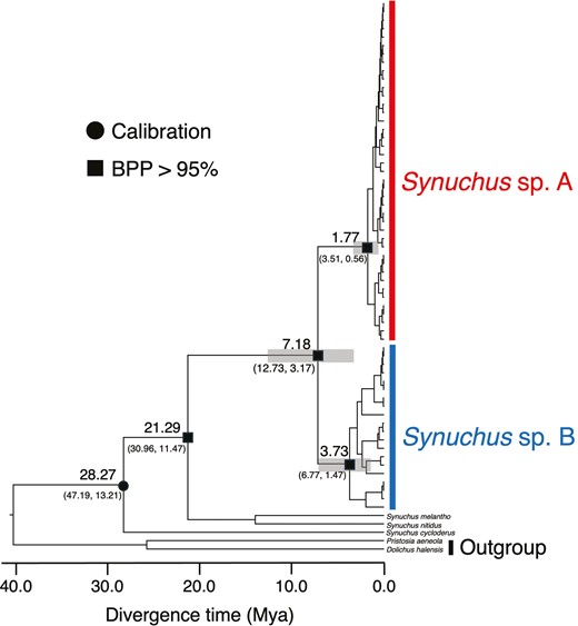
Divergence time estimation based on mitochondrial DNA COI sequences and nuclear DNA 28S sequences. Values above nodes indicate the estimated mean divergence time. Bars and values under nodes also indicate the 95% highest posterior density intervals of divergence time. The black circle indicates the secondary calibration point. The black squares indicate the >95% Bayesian posterior probability (BPP) of the major nodes.
Genetic diversity and geographical differentiation
Haplotype diversity and nucleotide diversity were greater in Synuchus sp. B than in Synuchus sp. A (Table 1). Synuchus sp. B showed greater intraspecific genetic differences (mean values and maximum values) than Synuchus sp. A (Table 2). The interspecific genetic distance ranged from 3.2% to 5.7%, and its mean value was 4.6% (Table 2). The minimum interspecific genetic distance (3.2%) was slightly greater than the maximum intraspecific genetic distance within Synuchus sp. B (3.1%).
Genetic diversity and demographic indices for Synuchus sp. A and Synuchus sp. B based on the mitochondrial DNA COI sequences.
| Species | N | Haplotype diversity | Nucleotide diversity | Tajima’s D | Fu’s Fs |
|---|---|---|---|---|---|
| Synuchus sp. A | 85 | 0.888 | 0.007 | −0.613 | −16.750* |
| Synuchus sp. B | 30 | 0.924 | 0.019 | 0.326 | 1.470 |
| Species | N | Haplotype diversity | Nucleotide diversity | Tajima’s D | Fu’s Fs |
|---|---|---|---|---|---|
| Synuchus sp. A | 85 | 0.888 | 0.007 | −0.613 | −16.750* |
| Synuchus sp. B | 30 | 0.924 | 0.019 | 0.326 | 1.470 |
*P < .001.
Genetic difference (p-distance) in each species and between Synuchus sp. A and Synuchus sp. B based on the mitochondrial DNA COI sequences.
| Comparison | Minimum | Mean | Maximum |
|---|---|---|---|
| Within Synuchus sp. A | 0.000 | 0.007 | 0.018 |
| Within Synuchus sp. B | 0.000 | 0.019 | 0.031 |
| Between Synuchus sp. A and Synuchus sp. B | 0.032 | 0.046 | 0.057 |
| Comparison | Minimum | Mean | Maximum |
|---|---|---|---|
| Within Synuchus sp. A | 0.000 | 0.007 | 0.018 |
| Within Synuchus sp. B | 0.000 | 0.019 | 0.031 |
| Between Synuchus sp. A and Synuchus sp. B | 0.032 | 0.046 | 0.057 |
For Synuchus sp. A, no significant correlation was detected between geographical and genetic distances (Mantel r = 0.06, P = .189; Fig. 5). In contrast, Synuchus sp. B showed a significant positive correlation between geographical and genetic distances (Mantel r = 0.58, P = .001; β = 0.01). Thus, geographical differentiation among the isolated populations occurred only in Synuchus sp. B (Fig. 5).
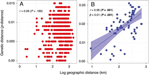
Relationship between geographical distance and genetic distance for Synuchus sp. A (A) and Synuchus sp. B (B). Values of geographical distance are log10-transformed. Genetic distance is the average pairwise distance (p-distance) of the mitochondrial DNA COI sequences. ‘r’ indicates Mantel r, and ‘β’ also indicates the slope of the regression. The line and coloured range in B are the results of linear regression analysis and indicate the regression line and 95% confidence interval. Statistically significant P-values are shown in bold.
Demographic analysis
Tajima’s D and Fu’s Fs showed negative values in Synuchus sp. A, and the latter was statistically significant (Table 1). On the contrary, these two indices were positive for Synuchus sp. B. The Bayesian skyline plot analyses revealed that the effective population size of Synuchus sp. A has increased since ~0.025 Mya, whereas that of Synuchus sp. B has decreased since ~0.05 Mya (Fig. 6). These results showed that Synuchus sp. A has experienced demographic expansion, whereas Synuchus sp. B has experienced demographic decline in the recent past.
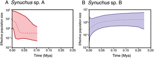
Bayesian skyline plots based on the mitochondrial DNA COI sequences for Synuchus sp. A (A) and Synuchus sp. B (B). Dotted lines indicate median values, and coloured ranges indicate the 95% highest posterior density intervals.
Distribution patterns and differences in the habitat environment
Synuchus sp. A was detected at 40 sites from Hokkaido to Kyushu, while Synuchus sp. B was detected at 12 sites from the mountainous area in central Honshu.
The area under the curve of the SDMs was 0.882 ± 0.020 (mean ± SD) for Synuchus sp. A and 0.974 ± 0.004 (mean ± SD) for Synuchus sp. B; thus, we could estimate the potential distribution area with high accuracy. The distribution probability for each species indicated that the potential distribution area of Synuchus sp. A was broad and covered the Japanese archipelago, whereas that of Synuchus sp. B was relatively narrow and restricted mainly to central Honshu (Fig. 7).
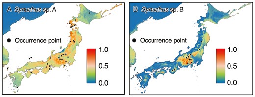
Estimated potential distribution area based on the species distribution models for Synuchus sp. A (A) and Synuchus sp. B (B). They are estimated by the Maxent with seven bioclimatic variables from WorldClim. The black dots indicate occurrence points. The bars indicate the predicted distribution probability.
In the PCA for climate conditions, the contribution of PC1 in the PCA was 42.8% and that of PC2 was 26.0% (Table 3). Therefore, ~70% of the entire dataset could be explained by PC1 and PC2. PC1 was positively correlated with temperature (BIO1, BIO5, BIO6, BIO9, BIO10, and BIO11) and negatively correlated with temperature difference (BIO4 and BIO7) (Table 3). In contrast, PC2 was positively correlated with precipitation in the cold and dry seasons (BIO14 and BIO17) and negatively correlated with precipitation in the warm and wet seasons (BIO13, BIO16, and BIO18) and with differences in temperature or precipitation (BIO3 and BIO15) (Table 3). The PCA plots of PC1 and PC2 revealed that Synuchus sp. A retained a broader ecological space than did Synuchus sp. B (Supporting Information, Fig. S5). PC1 and PC2 scores differed significantly between the two species (PC1: W = 339.5, P = .03; and PC2: W = 349.5, P = .02; Fig. 8).
Loading scores of the principal component analysis of the environmental differences based on temperature conditions and precipitation conditions.
| Bioclimatic variables | Principal component 1 (42.8%) | Principal component 2 (26.0%) | |
|---|---|---|---|
| Temperature | BIO1 (annual mean temperature) | 0.321 | −0.039 |
| BIO2 (mean diurnal range) | −0.170 | −0.240 | |
| BIO3 (isothermality) | −0.019 | −0.342 | |
| BIO4 (Temperature seasonality) | −0.266 | 0.208 | |
| BIO5 (maximum temperature of warmest month) | 0.281 | 0.028 | |
| BIO6 (minimum temperature of coldest month) | 0.336 | 0.005 | |
| BIO7 (temperature annual range) | −0.293 | 0.024 | |
| BIO8 (mean temperature of wettest quarter) | 0.112 | −0.170 | |
| BIO9 (mean temperature of driest quarter) | 0.305 | 0.167 | |
| BIO10 (mean temperature of warmest quarter) | 0.307 | 0.019 | |
| BIO11 (mean temperature of coldest quarter) | 0.326 | −0.069 | |
| Precipitation | BIO12 (annual precipitation) | 0.224 | −0.131 |
| BIO13 (precipitation of wettest month) | 0.207 | −0.255 | |
| BIO14 (precipitation of driest month) | 0.163 | 0.298 | |
| BIO15 (precipitation seasonality) | −0.041 | −0.437 | |
| BIO16 (precipitation of wettest quarter) | 0.156 | −0.285 | |
| BIO17 (precipitation of driest quarter) | 0.172 | 0.288 | |
| BIO18 (precipitation of warmest quarter) | 0.120 | −0.295 | |
| BIO19 (precipitation of coldest quarter) | 0.151 | 0.323 | |
The names of bioclimatic variables correspond to WorldClim. Absolute values of the loading scores (>0.25) are shown in bold.
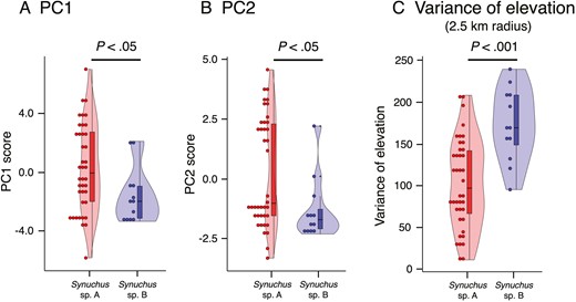
The environmental differences between the habitats of Synuchus sp. A and those of Synuchus sp. B. The values are based on principal component (PC) analysis (see Results) and calculation of the variance in elevation. A, differences in PC1 scores. B, differences in PC2 scores. C, differences in the variance of elevation (with a radius of 2.5 km). The results of Mann–Whitney U-tests and ANOVA are shown.
Variances in elevation also differed significantly between the two species (2.5 km radius: F = 16.98, d.f. = 1, P = .0001; Fig. 8) (5.0 km radius: F = 8.95, d.f. = 1, P = .0043; 10.0 km radius: F = 5.12, d.f. = 1, P = .0281; Supporting Information, Fig. S6).
DISCUSSION
We investigated the relationship among habitat environments, flight traits, and genetic differentiation process in the S. arcuaticollis species complex to test whether the species isolated in specific environments exhibits more degenerated flight traits and greater genetic differentiation. From our study, Synuchus sp. A, which had wide distribution and environmental ranges, was composed mostly of macropterous individuals and showed little genetic differentiation among populations. In contrast, Synuchus sp. B, which had a localized distribution and was restricted to specific environments, was apterous-monomorphic and showed high genetic differentiation among populations. These results are considered to support our hypothesis. In the following paragraphs, we will discuss each factor in detail.
The occurrence data and SDMs indicated that Synuchus sp. A was widely distributed (horizontally from Hokkaido to Kyushu and vertically from elevations of 30 to 1600 m a.s.l.), whereas Synuchus sp. B was restricted to the mountainous area in central Honshu (elevations of >1000 m a.s.l.) (Fig. 7; Supporting Information, Tables S1 and S2). The PCA of climate conditions revealed that Synuchus sp. B appears to have adapted to cooler environments with greater temperature differences (mainly based on PC1), more precipitation in winter, less precipitation in summer, and greater precipitation differences (mainly based on PC2) than Synuchus sp. A. In addition, the variance in elevation was significantly greater for Synuchus sp. B than for Synuchus sp. A (Fig. 8; Supporting Information, Fig. S6). In general, isolated and/or stable environments promote degeneration of flight ability in beetles (Darlington 1943, Den Boer et al. 1980, Roff 1990). Mountainous forests represent such environments (Darlington 1943, Southwood 1962, Roff 1990). From this knowledge, as expected, we confirmed the complete loss of hind wings in Synuchus sp. B, which inhabited highly isolated mountainous areas of central Honshu with specific climatic conditions. In contrast, Synuchus sp. A, distributed throughout the Japanese archipelago, inhabited a variety of environments and included mainly macropterous individuals.
In the case of carabid beetles, it is difficult to capture or observe flying individuals because most species are ground-dwelling (Shibuya et al. 2018). Thus, evaluating the dispersal ability by assessment of flight muscles and hind wings is important (Matalin 2003). All individuals in this study lacked distinct flight muscles; thus, most individuals of the S. arcuaticollis species complex seem to be flightless. However, the two species presented different patterns of hind wing polymorphism. Synuchus sp. A was polymorphic in the hind wing, indicating that this species is experiencing hind wing degeneration. In contrast, Synuchus sp. B is apterous-monomorphic and has completed hind wing degeneration. Although there have been no records of flying individuals of S. arcuaticollis and its related species, some previous studies have suggested that there are flight-capable individuals of other Synuchus species (Hori 2008, Shimizu et al. 2024). In addition, the important contribution of wind to insect dispersal was noted by Pasek (1988), and small, flightless insects could achieve long-distance dispersal via wind (Johnson 1957). In the case of carabid beetles, ‘hopping-fly’ behaviour, which involves low flight, using the wind and their hind wings, has been observed in flightless species (Thiele 1977), and Shibuya et al. (2017) noted that the ‘hopping-fly’ behaviour could occur in S. cycloderus. Based on this knowledge, it is possible that macropterous individuals of Synuchus sp. A might fly or flow with their hind wings, but Synuchus sp. B might not. Thus, Synuchus sp. A might have greater dispersal ability than Synuchus sp. B.
A single COI haplotype was shared by the individuals obtained widely from Hokkaido to Kyushu (Hap 4; Fig. 2; Supporting Information, Table S3) in Synuchus sp. A, with no significant pattern of isolation by distance. In contrast, Synuchus sp. B often had COI haplotypes unique to each site, with a significant pattern of isolation by distance. Divergence time estimation indicated that Synuchus sp. B was genetically differentiated earlier than Synuchus sp. A. In addition, demographic analyses revealed that Synuchus sp. A experienced demographic expansion, whereas Synuchus sp. B experienced demographic decline in the recent past. Furthermore, Synuchus sp. B presented greater genetic diversity than shown in Synuchus sp. A. These results suggest that range expansion and subsequent increase of gene flow among populations has occurred until recently and has resulted in a relatively homogeneous genetic structure in Synuchus sp. A. In contrast, it is possible that Synuchus sp. B has experienced range reduction and subsequent decrease of gene flow among populations for a long time, resulting in unique COI haplotypes in each area owing to geographical differentiation. Synuchus sp. A might have accomplished the expansion and gene flow owing to its wide habitable environment and rare dispersal by macropterous individuals. Conversely, gene flow in Synuchus sp. B might have been interrupted by isolation in mountainous areas and the complete loss of flight ability.
The proposed processes might have been influenced by the geological history of the Japanese archipelago. The Quaternary (from 2.58 Mya to the present) was an era with dynamic changes in the environment and cycles of glacial and interglacial periods (Rull 2008). These environmental changes are thought to have affected the diversification of insects in the Japanese archipelago (Tojo et al. 2017). The widening of the habitable environment and the presence of macropterous individuals might have allowed Synuchus sp. A to survive harsh climatic conditions through the Quaternary, adapt to warm climatic conditions after the Last Glacial Maximum (~0.021 Mya), and disperse from refugia. The intraspecific sharing of the same COI haplotype over a wide area, recent genetic divergence (from 1.77 Mya), and demographic expansion (from ~0.025 Mya) of Synuchus sp. A suggest that range expansion and gene flow among populations occurred in the Quaternary, and it might have worked in favour of prosperity in Synuchus sp. A. In contrast, the complete loss of flight ability, geographical differentiation, ancient genetic divergence (from 3.73 Mya), and demographic decline (from ~0.05 Mya) of Synuchus sp. B suggest the fragmentation and loss of gene flow among populations in the Quaternary. Thus, local populations of Synuchus sp. B might have been geographically isolated and shrunk after the Last Glacial Maximum because of the decreases in suitable habitats and gene flow among populations.
As discussed so far, isolation in discontinuous montane forests is likely to be a major factor contributing to the degeneration of flight ability and subsequent genetic differentiation among populations in Synuchus sp. B. However, we also need to be cautious, in that our results might be interpreted in an alternative scenario. We cannot rule out the possibility of ‘the opposite causal relationship’, which assumes that rapid degeneration of flight traits in Synuchus sp. B has restricted its distribution and habitat, leading to genetic differentiation. Results of phylogenetic analysis suggested that two species in S. arcuaticollis species complex are monophyletic. Thus, although it is unclear whether the common ancestral species retained flight muscle, it is also reasonable to assume that the ancestral species included macropterous individuals according to Roff’s (1986) hypothesis. There are several hypotheses about the degeneration process of hind wings in beetles (e.g. Den Boer et al. 1980, Shibuya et al. 2018); however, little is known about its evolutionary time scale. To confirm the order in the causal relationship between the isolation in discontinuous montane forests and the degeneration of flight ability, and their evolutionary time scales, it would be necessary to construct a phylogenetic tree with more species and to reconstruct the evolutionary processes for those factors.
We have discussed our results with an assumption that a small percentage of macropterous individuals of Synuchus sp. A might be able to fly. However, we cannot rule out the possibility that two species of the S. arcuaticollis species complex are unable to fly, because we cannot find individuals with distinct flight muscles and there are no records of flying individuals. In that case, these contrasting patterns of genetic differentiation and population dynamics might be explained by differences in distribution patterns and habitat environments. If so, Synuchus sp. A inhabit broad and continuous environments such that gene flows among populations might be likely to occur even if all individuals are flightless. To clarify which scenario is more plausible, it would be necessary to examine the presence or absence of flight muscles in more individuals. Some previous studies suggested that flight-capable individuals of the genus Synuchus occurred rarely (e.g. Inoue 1978, Hori 2008, Yamauchi and Ishitani 2020). Thus, it is possible that the sample size in this study (87 individuals) is too small to deduce the ability of Synuchus sp. A to fly. In addition, comparing genetic structures with those of related flight-capable species might be effective. Several flight-capable species, such as S. cycloderus, S. nitidus and S. dulcigradus, are sympatric with Synuchus sp. A throughout the Japanese archipelago (see Shimizu et al. 2024). Therefore, comparing the similarity of genetic structures between these species and Synuchus sp. A might provide key insights to clarify the validity of each scenario.
ACKNOWLEDGEMENTS
We thank T. Kagaya, S. Shibuya, and members of the Laboratory of Forest Zoology at The University of Tokyo for their comments and advice. We also thank G. Ueki and H. Yoshino for their technical advice. We are also grateful to R. Nakamura, S. Yamasaki, and K. Takeuchi for supplying samples and useful information and helping with the field survey, and to R. Sato and K. Hosokawa for making their sample collections available. A part of field survey was conducted with permission from The University of Tokyo Chichibu Forest.
CREDIT STATEMENT
Takashi Shimizu (Conceptualization, Data curation, Investigation, Formal analysis, Funding acquisition, Writing—original draft), Kôhei Kubota (Investigation, Supervision, Funding acquisition, Project administration, Writing—review & editing), Hiroshi Ikeda (Supervision, Funding acquisition, Project administration, Writing—review & editing).
CONFLICT OF INTEREST
None declared.
FUNDING
This study was supported by the Oki Islands UNESCO Global Geopark Academic Research Encouragement Project to T. Shimizu and the Japan Society for the Promotion of Science KAKENHI, grant numbers 21H04736 to K. Kubota and 23H02547 to H. Ikeda.
DATA AVAILABILITY
Additional Supporting Information will be available at the journal website. Sequence data are deposited in DNA Data Bank of Japan (DDBJ), and accession numbers are shown in Supporting Information, Table S3.
