


Abstract
Sampling k-mers is a ubiquitous task in sequence analysis algorithms. Sampling schemes such as the often-used random minimizer scheme are particularly appealing as they guarantee at least one k-mer is selected out of every w consecutive k-mers. Sampling fewer k-mers often leads to an increase in efficiency of downstream methods. Thus, developing schemes that have low density, i.e. have a small proportion of sampled k-mers, is an active area of research. After over a decade of consistent efforts in both decreasing the density of practical schemes and increasing the lower bound on the best possible density, there is still a large gap between the two.
We prove a near-tight lower bound on the density of forward sampling schemes, a class of schemes that generalizes minimizer schemes. For small w and k, we observe that our bound is tight when . For large w and k, the bound can be approximated by . Importantly, our lower bound implies that existing schemes are much closer to achieving optimal density than previously known. For example, with the current default minimap2 HiFi settings w = 19 and k = 19, we show that the best known scheme for these parameters, the double decycling-set-based minimizer of Pellow et al. is at most 3% denser than optimal, compared to the previous gap of at most 50%. Furthermore, when and the alphabet size σ goes to , we show that mod-minimizers introduced by Groot Koerkamp and Pibiri achieve optimal density matching our lower bound.
Minimizer implementations: github.com/RagnarGrootKoerkamp/minimizers ILP and analysis: github.com/treangenlab/sampling-scheme-analysis.
1 Introduction
For over a decade, k-mer sampling schemes have served as a ubiquitous first step in many classes of bioinformatics tasks. By sampling k-mers in a way which ensures that two similar sequences will have similar sets of sampled k-mers, sampling schemes enable methods to bypass the need to compare entire sequences at the base level and instead allow them to work more efficiently using the sampled k-mers.
Local sampling schemes satisfy a window guarantee that at least one k-mer is selected out of every window of w consecutive k-mers. Most schemes used in practice, such as the random minimizer scheme (Schleimer et al. 2003, Roberts et al. 2004), are forward schemes that additionally guarantee that k-mers are sampled in the order in which they appear in the original sequence. These properties are particularly appealing since they guarantee that no region is left unsampled.
As the purpose of these schemes is to reduce the computational burden of downstream methods while upholding the window guarantee, the primary goal of most new schemes is to minimize the density, i.e. the expected proportion of sampled k-mers. Over the past decade, many new schemes have been proposed that obtain significantly lower densities than the original random minimizer scheme.
For example, there are schemes based on hitting sets (Orenstein et al. 2016, Marçais et al. 2017, 2018, DeBlasio et al. 2019, Ekim et al. 2020, Pellow et al. 2023, Golan et al. 2024), schemes that focus on sampling positions rather than k-mers (Loukides and Pissis 2021, Loukides et al. 2023), schemes that use an ordering on t-mers (t < k) to decide which k-mer to sample (Zheng et al. 2020, Groot Koerkamp and Pibiri 2024), and schemes that aim to minimize density on specific input sequences (Zheng et al. 2021b, Hoang et al. 2022). All of these improvements notwithstanding, it is still unknown how close these schemes are to achieving minimum density.
A trivial lower bound on density given by the window guarantee is , and recently Groot Koerkamp and Pibiri (2024) improved the bound of Marçais et al. (2018) from to . However, for many practical values of w and k, there is a sizeable gap between these lower bounds and the density of existing schemes. This raises the question whether schemes with density much closer to exist, but have not been found yet, or whether existing schemes are already very close to optimal and it is the lower bound that needs improvement. Our new lower bound closes most of the gap, and thus answers this question: Indeed, especially for , the best existing schemes have near-optimal density in many cases. This allows future research to focus on improving other sampling scheme metrics, such as the conservation described by Edgar (2021) and Shaw and Yu (2022).
1.1 Contributions
Main lower bound theorem. We prove a novel lower bound on the density of forward schemes that is strictly tighter than all previously established lower bounds for all w, k, and alphabet size σ:
We prove that this bound can be extended to work for more general classes of sampling schemes, such as the local schemes described by Marçais et al. (2018) and the multi-local schemes described by Kille et al. (2023).
Comparison with optimal schemes for small parameters. We show that our lower bound is tight for some small w, k, and σ by using an integer linear program to construct schemes whose density matches our lower bound. This marks the first time that there is an analytical description of a tight minimum density of any forward scheme. We conjecture that when , there exist schemes with density matching our lower bound.
Comparison with practical schemes for large parameters. To show that our bound is significantly closer to the density achieved by existing schemes compared to previous lower bounds, we replicate the benchmark from Groot Koerkamp and Pibiri (2024) for a selection of w and k (Fig. 3). For example, with the default minimap2 (Li 2018) HiFi settings w = 19 and k = 19, the lower bound goes up from 50% of the density achieved by the double decycling based method to 97% of the achieved density (Table 1).
Minimum densities achieved by existing sampling schemes for default parameters of frequently-used bioinformatics methods (σ = 4)a
| Application | (w, k) | Random | Best | Lower bound | Gap (%) | |||
|---|---|---|---|---|---|---|---|---|
| Scheme | Density | |||||||
| Kraken2 | (5, 31) | 0.333 | Mod-mini | 0.226 | 0.200 | 0.222 | 12.8 | 1.6 |
| SSHash | (12, 20) | 0.154 | Mod-mini | 0.120 | 0.083 | 0.108 | 43.9 | 10.9 |
| minimap2, hifi | (19, 19) | 0.100 | dbl decycling | 0.079 | 0.053 | 0.077 | 50.1 | 2.7 |
The gap percentage describes the how much larger the lowest achieved density is than the lower bound and is calculated as , where for the old gap and for the new gap. While Groot Koerkamp and Pibiri (2024) showed that is also a lower bound, is tighter for all of the parameter choices in the table. For SSHash (Pibiri 2022), we show parameters used for indexing a single human genome.
Analysis of the mod-minimizer. Finally, our new lower bound implies that the mod-minimizer scheme (Groot Koerkamp and Pibiri 2024) is optimal when and σ is large. Indeed, for the ASCII alphabet (σ = 256), the mod-minimizer scheme density is consistently within 1% of the lower bound when (Supplementary D, Fig. S4).
2 Background
Notation. We begin by defining some necessary notation, as well as definitions of mathematical concepts that will be used throughout the work. We use to refer to the set . The alphabet is denoted by Σ and has size , with σ = 4 for DNA. The expression indicates that a divides b. The summation is over all positive divisors a of b. We use for the remainder (in ) of a after dividing by m and we use to indicate that a and b have the same remainder modulo m. Given a string W, ) refers to the substring of W containing the characters at 0-based positions i up to j − 1 inclusive. For two strings X and Y, XY represents the concatenation of X and Y.
Classes of sampling schemes. There are multiple established classes of sampling schemes. We begin by drawing a distinction between schemes with and without a window guarantee that guarantees that at least one every w k-mers is sampled. While schemes without a window guarantee, such as fracminhash (Irber et al. 2022), are often efficient to compute, the lack of a guarantee on the distance between sampled k-mers makes them ineffective or inefficient for certain tasks such as indexing and alignment. Indeed, we only consider schemes with a window guarantee:
A (w, k)-local scheme with window guarantee w and k-mer size k on an alphabet Σ corresponds to a sampling function .
In other words, given a window of characters (w consecutive k-mers), the output of the sampling function f(W) is an integer in which represents the index of the sampled k-mer in W. Recently, Kille et al. (2023) proposed a generalization of (w, k)-local schemes which samples at least s k-mers out of every w instead of at least 1 and we extend our results to these more general schemes in Supplementary A.
Local schemes have no restrictions on which of the w k-mers can be selected for each window, but forward schemes are a subset of local schemes that enforce the restriction that they never select a k-mer which occurs before a previously selected k-mer.
The density of a sampling scheme f is defined as the expected proportion of sampled positions from an infinite, uniformly random string.
For a further background on types of sampling schemes, we refer to Shaw and Yu (2022), Zheng et al. (2023), Groot Koerkamp and Pibiri (2024), and Ndiaye et al. (2024).
De Bruijn graphs. Let denote the complete De Bruijn graph of order n, which has as vertices all strings of length n, , and edges between vertices that overlap in n − 1 positions, . When σ is clear from the context or irrelevant for a particular discussion, it is omitted. It is worth noting that the vertices of correspond to edges of Bn.
For each string s of length n, the n rotations of s induce a pure cycle in Bn consisting of (up to) n vertices cyclically connected by edges. Note that when s is repetitive, e.g. a single repeated character or some other repeated string, the length of the cycle will be a divisor of n. These pure cycles are also called necklaces. The set of necklaces of length n corresponds to a partitioning of the vertices of Bn into a vertex-disjoint set of pure cycles. We use to refer to this set of pure cycles of Bn, and for , we write for the number of vertices in the cycle.
Charged contexts. The context of a window of length in a sequence is the set of preceding windows that influences whether the current window samples a new position.
For a local scheme to select a new position, none of the previous w − 1 windows may have selected the same k-mer as the current window. As a result, the context for local schemes consists of characters: the current window of w k-mers as well as the w − 1 windows preceding the current window.
For a forward scheme, however, as soon as a window samples a different position than the preceding window, this position must be a new position. Thus, one needs only to consider the context of two consecutive windows of w k-mers, for a total of w + k characters.
When a sampling scheme selects a new position for the last window in a context, the context is charged. Marçais et al. (2017) showed that the density of a scheme f can be defined as the proportion of contexts which are charged. In the case of forward schemes, each edge in represents a context, and the charged contexts are the edges (u, v) for which .
Universal hitting sets. In 2021, Zheng et al. (2021a) related the density of forward and local schemes to the concept of universal hitting sets (UHS). A -UHS is defined as a set of -mers U such that any sequence of w adjacent -mers must contain at least one -mer from U. Theorem 1 of Zheng et al. (2021a) showed that when k = 1, one can use the minimum size of a -UHS to bound the density of -forward schemes, and the minimum size of a -UHS to bound the density of a -local scheme.
3 Theoretical results
In this section, we prove our main result: an improved lower bound on the density of forward sampling schemes. We first generalize some existing theorems to arbitrary w and k (Sections 3.1 and 3.2), after which our main theorem follows in Section 3.3.
3.1 A lower bound on the size of a -UHS
We begin by considering a -UHS. A -UHS is equivalent to a vertex cover in , i.e., a subset of vertices such that each edge in is adjacent to at least one vertex in the subset. Lichiardopol (2006) used the fact that for every cycle C, at least of its vertices must be in a vertex cover, and obtained a lower bound on the size of a vertex cover by partitioning into its pure cycles. We naturally extend this argument to obtain a lower bound on the cardinality of a -UHS for any .
□
Figure 1b provides a depiction of a minimum (2, 4)-UHS as well as the pure-cycle partitioning of B4 on a binary alphabet. Notably, the pure cycle has three vertices in the UHS, even though the lower bound given by Proposition 4 only requires it have 2. This is an example where the lower bound is not tight.
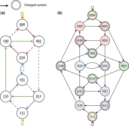
(a) A De Bruijn graph B3 corresponding to a minimum density -forward scheme. The underlined characters in each vertex represent the 2-mer that is selected for that window. The solid edges represent the charged contexts and the edge colors represent the pure cycles in B4 (not in B3 itself). For characters ci, each edge in B3 corresponds to the vertex in B4. (b) The corresponding -UHS in B4. The vertices are partitioned by color, representing the pure-cycles. The 2-mer(s) selected in each context are underlined. The vertices with a double border represent the charged edges in B3 in (a) and the corresponding (2, 4)-UHS. Each pure cycle c has at least vertices in the UHS.
For certain values of w and , such as when is prime or w = 2 and is odd, Proposition 4 can be simplified to remove the summation and ceil function (Supplementary B).
Proposition 4 is the core of the proof of Theorem 1 and already has the right structure. The remainder of this section translates this result on universal hitting sets to a result on the density of sampling schemes.
3.2 A connection between sampling scheme density and UHS size
Zheng et al. (2021a, Theorem 1) showed a connection between universal hitting sets and the density of sampling schemes when k = 1. We naturally extend their result to for both local schemes (Lemma 5) and forward schemes (Corollary 6).
Then, Cf is a -UHS.
Proof. For the sake of a contradiction, suppose there is a walk of length w in the De Bruijn graph of order , say , that avoids cf Let S be the spelling of the walk, i.e., the sequence of length such that . Since and S contains , this implies that on the last -mer of (i.e. ), f selects an index in S which has already been picked.
Since and , the first window that selects position j must begin at an index . Therefore, the context is charged, as f selects a previously unselected position when applied to its last -mer. By definition, , contradicting our supposition and therefore Cf is a -UHS. □
Identically, one can consider contexts for a (w, k)-forward scheme f, which requires only verifying that the selection for a window of length is distinct from the selection for the previous window. Therefore, the length of a context for forward f is only w + k. As above, every w contexts must have at least one charged context, leading to the following conclusion:
If f is a (w, k)-forward scheme and Cf is its corresponding set of charged contexts, defined as, then Cf is a-UHS.
As all contexts of a particular length are equally likely to occur in an infinite, uniform random string, the proportion of charged contexts corresponds to the density of the sampling scheme (Marçais et al. 2017), i.e. , where for forward schemes and for local schemes. An example of the charged contexts of a (2, 2)-forward scheme and the corresponding UHS is depicted in Fig. 1.
3.3 Lower bounds on local and forward scheme density
We are now ready to state and prove our main theorem.
Proof. Due to Corollary 6 and Marçais et al. (2017), we can see that a (w, k)-forward sampling scheme of density implies a -UHS of size . By Proposition 4, this implies that every forward sampling scheme has a density of at least , and hence follows.
For any p that divides w + k, we have, with strict inequality when p = 1 and w > 1. Substituting this in , the middle inequality follows directly using the identity that counts the number of strings of length w + k partitioned by their shortest period.
The last inequality follows directly from . □
As shown in Section 4, is a tight bound for many small cases. Since its formula is somewhat unwieldy, can be used as an approximation that quickly approaches (Fig. 2). Simple arithmetic shows that both and improve the previous lower bound of of Groot Koerkamp and Pibiri (2024).
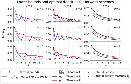
Comparison of forward scheme lower bounds and optimal densities for small w, k, and σ. Optimal densities were obtained via the ILP and are plotted as black circles that are solid when the optimal density matches our lower bound, , and hollow otherwise. Each column corresponds to a parameter being fixed to the lowest non-trivial value, i.e., σ = 2 in the first column, w = 2 in the second column, and k = 1 in the third column. Note that the x-axis in the third column corresponds to w, not k.
Given a (w, k)-local scheme fk, we can construct a -local scheme of the same density by ignoring the last characters in each window, i.e. . This directly implies (Zheng et al. 2021a). It follows that the minimum density of a (w, k)-local or forward scheme is monotonically decreasing as k increases. However, as can be seen in Fig. 2, is not a monotonically decreasing function. The local maxima appear to be at , which motivates the following improved lower bound.
4 Empirical tightness of our bounds
Here, we compare our bounds and to existing lower bounds. Further, we show how tight these bounds are for small w, k, and σ by searching for optimal schemes via an integer linear programming (ILP) formulation. We also show how close existing sampling scheme densities are to for practical choices of w, k, and σ. Finally, we show when the recently described mod-minimizer scheme (Groot Koerkamp and Pibiri 2024) achieves optimal density as .
ILP description. We use an ILP to search for minimum density forward sampling schemes. In short, we use a single integer variable for every window W of length (corresponding to a vertex in ) that indicates the position of the chosen k-mer, and a single boolean variable for each edge in that indicates whether the corresponding context is charged. On each edge, we require that the scheme be forward. The objective function is to minimize the number of charged edges. To reduce the search space, we add an additional constraint corresponding to our lower bound by requiring that for each pure cycle of length in , at least of the corresponding edges in are charged. Further details, including the ILP formulation for local schemes, can be found in Supplementary C.
Comparison against optimal schemes for small k. We used Gurobi (Gurobi Optimization, LLC 2024) to solve the ILP for all combinations of w, k, and σ such that , and for both forward and local schemes and limited the runtime for each instance to 12 h on 128 threads. All results are reported in in Supplementary D, Table S2. While the additional constraint on pure cycles corresponding to significantly sped up the search, for most large w, k, and σ, the ILP failed to terminate with an optimal solution in the allotted time. As a result, we restrict most of our analysis to the following three cases: fixed alphabet size σ = 2, fixed window size w = 2, and fixed k-mer size k = 1 (Fig. 2).
For all where (including when k = 1), the minimum density exactly matches our lower bound . Additionally, when σ = 2 and w = 2, the minimum density was equal to .
Comparison against existing schemes for large k. Using a sequence of 10 million random characters over alphabet size σ = 4, we approximated the density of recent sampling schemes using the benchmarking implementation from Groot Koerkamp and Pibiri (2024). To compare each density to the particular proportion of selected k-mers on a genomic sequence, we also ran all sampling schemes on the human Y chromosome (Rhie et al. 2023) after removing all non-ACTG characters. The densities of the best performing methods, Miniception (Zheng et al. 2020), double decycling-set-based minimizers (Pellow et al. 2023), and mod-minimizers (Groot Koerkamp and Pibiri 2024) are plotted in Fig. 3 along with random minimizers and lower bounds.
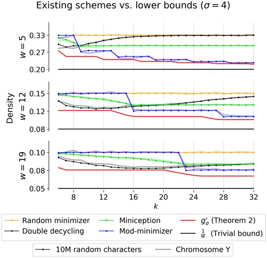
Comparison of existing schemes to lower bounds with practical parameters. Densities are calculated by applying each scheme to a random sequence of 10 million characters over an alphabet of size σ = 4 (dotted lines) and are compared with the corresponding proportion of sampled k-mers on the human Y chromosome (Rhie et al. 2023) (soft lines). The mod-minimizer uses parameter r = 4, and miniception uses parameter . The window sizes 5 and 19 are the default window sizes for Kraken2 (Wood et al. 2019) and minimap2 (-ax hifi) (Li 2018), respectively. For SSHash, w = 12 was the window size used when indexing the human genome (Pibiri 2022).
The ratio between the minimum achieved densities and lower bounds for a selection of (w, k) pairs used by existing k-mer-based methods are presented in Table 1. Additional results for and are provided in in Supplementary D, Fig. S4.
Thus, the mod-minimizer has density equal to the lower bound provided by Theorem 1 when σ goes to and w and are fixed.
In practice, for σ = 256 the mod-minimizer scheme is within 1% from optimal when (Supplementary D, Fig. S4). When σ = 4 (Fig. 3), a t > 1 must be used, causing the density plot to ‘shift right’ compared to the lower bound. Because of that, the mod-minimizer does not quite match the lower bound for practical values of σ.
5 Discussion
5.1 Conjecture on when our lower bound is tight
Analytically, it is clear that is much larger than . In all cases, is nearly tight, if not completely. In particular, our bound is tight for all 40 tested parameter sets where , leading us to our conjecture:
For any w and k satisfying , there exists a (w, k)-forward sampling scheme f such that.
While the minimum size of a decycling set, i.e., a -UHS, is well known to be (Mykkeltveit 1972), very little is known about the minimum size of a -UHS for finite w. In addition to providing the minimum density of a (w, k)-forward scheme for , proving Conjecture 1 would also determine the minimum size of a -UHS when .
5.2 Existing schemes are nearly optimal when or σ is large
A natural investigation which follows our proposed lower bound is to determine the gap between and current forward scheme densities. Previously, the gap between known densities and lower bound was rather large, making it unclear how much more the density could be reduced.
In Table 1, we observe that existing schemes are already within 11% from the optimal density for practical values of w and k across different applications, and in many cases are even within 3% of the optimal density. In Fig. 3, we see that this difference holds not just for the specific (w, k) in Table 1, but for most . This is much more informative than the previous lower bound of , which implied that most current schemes are at most 50% denser than optimal for many of the parameters in Fig. 3.
For alphabets much larger than DNA , such as the ASCII alphabet (σ = 256), we observe that when , the mod-minimizer scheme recently proposed by Groot Koerkamp and Pibiri (2024) is at most 1% denser than optimal and furthermore, we show that it is optimal as . This makes the mod-minimizer scheme the first practical scheme for which there exist finite parameters k and w for which it is close to optimal.
5.3 Tightening the bound for small k
Our new bound for forward schemes always improves over and appears tight when . This leads to an increasingly close bound for as k increases, but leaves a large gap when . A better understanding of these small cases will be necessary to obtain a tight lower bound for all w and k. Based on Supplementary D, Figs. S3 and S4, one might conjecture that the double decyling-set-based methods of Pellow et al. (2023) are near-optimal, but subsequent work such as the greedy minimizer (Golan et al. 2024) has shown better schemes are possible. From Fig. 2, we already know that our lower bound is not always tight, so this leaves the question:
Open problem 1. How close can practical sampling schemes get to the density given by our lower bound?
5.4 Extending the bound to local schemes
For local schemes, though, our bound appears much less tight. We identified eight sets of where local schemes can obtain lower densities than their forward counterparts. In all cases, however, the difference between the local and forward densities was minuscule, with the largest difference of being found for where the density decreased from 0.375 to 0.371 (Supplementary D, Table S2). Nevertheless, for some parameters, local schemes are able to achieve densities lower than our lower bound for forward schemes. Given the trend observed in Supplementary D, Table S2, we arrive at our final open problem:
Open problem 2. How much lower can the density of a (w, k)-local scheme be compared to a (w, k)-forward scheme?
Acknowledgements
We thank Giulio Ermanno Pibiri, Nicolae Sapoval, and our reviewers for their suggestions which helped improve the manuscript.
Supplementary data
Supplementary data are available at Bioinformatics online.
Conflict of interest: None declared.
Funding
This work was supported by the National Library of Medicine Training Program in Biomed-ical Informatics and Data Science [T15LM007093 to B.K.]; in part, the National Institute of Allergy and Infectious Diseases [P01-AI152999 to B.K. and T.J.T.], National Science Foundation (NSF) awards [IIS-2239114 and EF-2126387 to T.J.T]. R.G.K. is supported by ETH Research Grant ETH-1721-1 to Gunnar Rätsch.
Data availability
No new data were generated or analysed in support of this research.
References
Author notes
Bryce Kille and Ragnar Groot Koerkamp Equal contribution.

