


Abstract
There are compelling reasons to test compositional hypotheses about microbiome data. We present here linear decomposition model-centered log ratio (LDM-clr), an extension of our LDM approach to allow fitting linear models to centered-log-ratio-transformed taxa count data. As LDM-clr is implemented within the existing LDM program, this extension enjoys all the features supported by LDM, including a compositional analysis of differential abundance at both the taxon and community levels, while allowing for a wide range of covariates and study designs for either association or mediation analysis.
LDM-clr has been added to the R package LDM, which is available on GitHub at https://github.com/yijuanhu/LDM.
1 Introduction
Microbiome association studies detect taxa that are most strongly associated with the trait of interest (e.g. a clinical outcome or environmental factor), which are then used as microbial biomarkers for prognosis and diagnosis of a disease or microbial targets (e.g. pathogenic or probiotic bacteria) for drug discovery. Data derived from 16S amplicon or metagenomic sequencing are generally summarized in a taxa count table. However, since the total sample read count (library size) is an experimental artifact, only the relative abundances of taxa can be measured, not their absolute abundances. Consequently, microbiome data are compositional, meaning that a change in one taxon’s relative abundance necessitates a counterbalancing change in the relative abundance of (at least one) other taxa. The compositional null hypothesis tested for a taxon posits that the ratios of taxon relative abundances are constant across varying trait values. This hypothesis is frequently expressed in terms of parameters describing log-transformed data; the centered log ratio (clr), which centers the log relative abundance of each taxon by the sample mean log relative abundance of all taxa is most frequently used (Aitchison 1986). Since zero count data cannot be log-transformed, it is customary to add a pseudocount, usually 0.5 or 1, to the zeros or all entries in the taxa count table (Aitchison 1986, Lin and Peddada 2020).
We previously developed the linear decomposition model (LDM) (Hu and Satten 2020, Hu et al. 2021, Zhu et al. 2021, Hu et al. 2022b, Yue and Hu 2022, Zhu et al. 2022) for testing hypotheses about the microbiome. Initially, LDM was designed for testing the null hypothesis that the relative abundance at a given taxon remains constant as the trait changes; this hypothesis could also be tested using arcsin-root-transformed relative abundance data. Later, LDM was extended to accommodate presence-absence data (Hu et al. 2021). LDM is based on a linear model that regresses taxon data on traits/covariates, using a permutation procedure for inference. The linear model and permutation-based inference render LDM highly versatile, making it suitable for a wide variety of analyses (e.g. association, mediation), taxon data scales (e.g. relative abundance or presence-absence), trait types (e.g. continuous, discrete, multivariate, and time-to-event), and sample structures (e.g. matched sets, clustered data). Further, LDM gives a unified taxon- and community-level analysis.
LinDA (Zhou et al. 2022), a recently published method for compositional analysis of microbiome data, adopts a linear model for clr-transformed taxon data. It has demonstrated better FDR control and higher sensitivity than many existing compositional methods, including ANCOM-BC (Lin and Peddada 2020), ALDEx2 (Fernandes et al. 2014), metagenomeSeq (Paulson et al. 2013), and MaAsLin2 (Mallick et al. 2021). However, LinDA bases its inference on asymptotic distributions, which may not be appropriate for small sample sizes, small numbers of taxa, and complex data structures. Furthermore, LinDA is not applicable to multivariate traits or time-to-event (survival) outcomes and cannot be used for testing community-level hypotheses.
In this paper, we present LDM-clr, an extension of LDM for compositional analysis that incorporates clr-transformed data. Because the parameters tested in the compositional hypothesis involve more than one taxon, some changes to LDM are required, as described herein. The resulting tests still inherit the aforementioned features of LDM, as summarized in Supplementary Fig. S1.
2 Materials and methods
Denote the least-square estimators of and obtained using the LDM by and , respectively. In order to obtain inference on individual taxa, we follow the approach in LOCOM (Hu et al. 2022a) and assume that the majority (i.e. more than half) of the taxa are null taxa. This assumption has been frequently adopted in compositional methods (e.g. Kumar et al. 2018, Brill et al. 2022, Hu et al. 2022a). With this assumption, we expect that the median of the s, denoted by , will correspond to a taxon that is null. If this is the case, then we expect if taxon j is also null. When is a vector, the median is calculated in an element-wise manner.
When the number of taxa J is small, may contribute considerable variability. In this case, we still use (3), but use the value of and hence calculated for each permutation replicate. Thus, the total sum-of-squares in the denominator of (3) is different for each replicate; the “missing” variability corresponds to the variability in . Similarly, the global test in LDM-clr sums numerators and denominators in (3) separately. The change in total variability across replicates does not affect the validity of the test because it is permutation-based. In our simulations, the use of from each permutation replicate was only necessary for .
Like LOCOM and LDM-clr, LinDA also bases inference on although LinDA refers to as a “bias” rather than recognizing that the regression coefficients in models (1) and (2) are simply different. LinDA estimates the “bias” using the mode of the s, leading to the odd conclusion (in their framework) that the mode be used to estimate the mean of the values. Still, in our framework, using the mode in place of the median when calculating is attractive in some settings, and is offered as an option in LDM-clr.
3 Results
3.1 Simulation studies
We evaluated LDM-clr using the same set of simulation settings used to assess LinDA (Zhou et al. 2022): S0C0 (a binary trait), S0C1 (a continuous trait), S0C2 (a binary trait with two confounders), S1C0 (zero-inflated absolute abundances), S2C0 (correlated absolute abundances.), S3C0 (Gamma abundance distribution), S4C0 (small number of taxa), S5C0 (small sample size), S6C0 (10-fold difference in library size), S7C0 (Negative-Binomial abundance distribution), S8.1C0 (pretreatment and posttreatment comparison within subjects), and S8.2C0 (replicate sampling, specifically, 2 replicates for 25 subjects in the case with sample size 50, and 4 replicates for 50 subjects in the case with sample size 200). We applied LDM-clr using both the mode and median as , referred to as LDM-mode and LDM-median, respectively, for testing individual taxa and the entire community. Additionally, we applied LinDA for testing individual taxa only.
First, we successfully replicated the results of LinDA as reported in Zhou et al. (2022). In S4C0 (Fig. 1, left), where LinDA yielded inflated FDR due to a small number of taxa, LDM-mode and LDM-median controlled the FDR as they adjusted for the uncertainty in the value of . In S8.2 (Fig. 1, right), where replicate samples were present, LDM-mode and LDM-median yielded higher sensitivity than LinDA, with an increase of up to 9%, which is attributable to our permutation-based inference. In general, whenever LinDA controlled the FDR, LDM-mode and LDM-median also controlled the FDR. When LinDA had inflated FDR, such as in S4C0 (Fig. 1, left), S3C0 (Supplementary Fig. S7), and S6C0 (Supplementary Fig. S9), LDM-mode and LDM-median controlled the FDR or had less inflated FDR. The only exception is in S3C0 (Supplementary Fig. S7), where LDM-median had a more inflated FDR than LinDA. With sparse signals, use of the median for exhibited better sensitivity than use of the mode. Conversely, with dense signals, the mode-based estimator outperformed the median-based estimator. However, in both cases, using the median led to better power for community-level tests than using the mode (Supplementary Fig. S12).
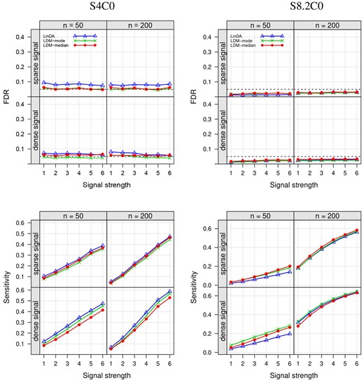
Empirical FDR and sensitivity at the nominal FDR level of 0.05 (black dashed line) in the S4C0 setting (with a small number of taxa, i.e. ; in other settings, ) and the S8.2C0 setting (with replicate sampling). The scenarios with “sparse” and “dense” signals have signal densities 5% and 20%, respectively. The “signal strength” values labeled as correspond to six combinations of effect sizes at differentially abundant taxa with increasing strength; see more detail in the “Detailed setups for numerical studies” section of Zhou et al. (2022). All results here as well as in other figures were based on 1000 replicates of data.
3.2 Compositional analysis of the aGVHD data
We analyzed the 16S rRNA sequencing data on acute graft-versus-host disease (aGVHD) (Jenq et al. 2015), which originally consisted 2436 operational taxonomic units (OTUs) across 94 subjects. Following the guidelines in Zhou et al. (2022), we removed subjects with library sizes <1000 and excluded OTUs found in fewer than 10% subjects, resulting in a final dataset comprising 89 subjects and 304 OTUs for our analysis. We tested the association of the gut microbiome with two survival outcomes separately: the overall survival and the time to stage-III aGVHD, with censoring rates of 52.3% and 42.0%, respectively. Both analyses were adjusted for age and gender.
We previously demonstrated in Hu et al. (2022b) that testing each taxon for association with a survival outcome using the Cox proportional hazard model performs poorly in the microbiome setting that typically has sparse count data and small sample sizes. We also established in Hu et al. (2022b) that the association between a taxon and the censored survival time can be tested by first converting the censored survival times into Martingale or deviance residuals generated from the Cox model that uses potentially confounding variables (such as age and gender in this case) as covariates while excluding the taxon data, and then using the LDM that regresses the taxon relative abundances on the Martingale or deviance residuals. LDM also provides a combination test that integrates the results from analyzing the two residuals (Martingale and deviance). LDM-clr inherits these features, enabling testing of clr-transformed data with censored survival times at both taxon and community levels. Using the same approach, we can also apply LinDA to test censored survival times by manually calculating the Martingale or Deviance residual for these data, and then treating it as a covariate. However, LinDA does not support combination tests or community-level tests.
The results of our analyses are summarized in Table 1. For the time to stage-III aGVHD, LDM-mode detected 13 associated OTUs at the nominal FDR level of 5%, while LinDA detected 16, using the Martingale residual. The 16 OTUs detected by LinDA include all 13 OTUs detected by LDM-mode, and the 3 OTUs detected by LinDA but not LDM-mode are among the bottom 4 OTUs (i.e. the least significant) in the list of LinDA detections. As our simulation results indicate that LDM-clr generally has better control of FDR, we belive that these three OTUs are likely false positives. Both methods detected 0 associated OTUs using the Deviance residual, demonstrating a significant variability in results when choosing which residual to use a priori. Fortunately, LDM-mode offers a combination test that detected eight associated OTUs. The community-level P-values generated by both LDM-median and LDM-mode were all small, aligning with the detection of associated OTUs. For the overall survival, LDM-mode detected three OTUs, consistent with its small community-level P-value, while LinDA detected none.
Results from compositional analysis of the aGVHD data.a
| Outcome | Method | Number of detected OTUs | Community-level P-value | ||||
|---|---|---|---|---|---|---|---|
| Martingale | Deviance | Combined | Martingale | Deviance | Combined | ||
| Time to aGVHD | LDM-median | 0 | 0 | 0 | 0.00840 | 0.0282 | 0.0106 |
| LDM-mode | 13 | 0 | 8 | 0.00440 | 0.0180 | 0.00600 | |
| LinDA | 16 | 0 | NA | NA | NA | NA | |
| Overall survival | LDM-median | 0 | 0 | 0 | 0.0288 | 0.0990 | 0.0350 |
| LDM-mode | 3 | 0 | 0 | 0.0150 | 0.0542 | 0.0192 | |
| LinDA | 0 | 0 | NA | NA | NA | NA | |
The nominal FDR level is 5%. “NA” indicates that the test is not available.
4 Discussion
Recently, Zhou et al. (2022) have proposed LinDA, a linear model for clr-transformed data that has some similarities with LDM-clr. One major difference between LinDA and the LDM family is that LinDA uses asymptotic distributional assumptions, so that P-values are calculated using normal (or t distributions in the case of small sample sizes) for independent samples; inference in LDM is permutation-based. Additionally, for correlated samples, LinDA uses asymptotic results for the linear mixed-effect model, which may fail if the distributional assumptions do not hold; in contrast, LDM-clr handles sample clustering by a distribution-free approach (Zhu et al. 2021). Further, inference in LinDA does not account for variability in , which we find is important when the number of taxa is small. In general, permutation-based tests take more run time than tests that are based on asymptotic inference; however, because LDM is based on the simple linear regression and adopts a sequential stopping rule, the computation time is still manageable for datasets that consist of hundreds of samples and taxa. We have performed more benchmarking of LDM-clr and LinDA using the benchdamic framework (Calgaro et al. 2023); these results are presented in Supplementary Text S1 and corroborate our observations in the simulation studies.
Another difference between LinDA and LDM is that LDM provides a unified framework of taxon-level and community-level tests, ensuring coherence between their results; LinDA does not support community-level tests. Specifically, the LDM test statistic for the community-level test is a ratio, with numerator and denominator given by the sum of the taxon-specific F-statistic numerators and denominators, respectively. When the number of taxa J is large enough that the variability in can be ignored, the LDM-clr global test statistic is equal to the PERMANOVA test statistic based on Aitchison’s distance (the Euclidean distance of clr-transformed data) applied to data [defined just after (3)]. Here we note that the Freedman-Lane permutation scheme used by the LDM and PERMANOVA-FL functions in the R package LDM actually gives slightly higher power than that attained by the implementation of PERMANOVA in the R package vegan (Hu and Satten 2020). Even when the variability in is accounted for, LDM-clr still produces test statistics that are similar to PERMANOVA based on . We note that comparison of LDM-clr and PERMANOVA using Aitchison’s distance is appropriate as this distance is considered the appropriate metric for community-level tests in compositional analysis of microbiome data (Gloor et al. 2017). Thus, we are confident that LDM-clr provides a useful addition to the growing list of methods for compositional analysis of complex microbiome data.
Supplementary data
Supplementary data are available at Bioinformatics online.
Conflict of interest
None declared.
Funding
This research was supported by the National Institutes of Health award [R01GM141074 to Y.-J.H. and G.A.S.].

