


Abstract
With the advancements of high-throughput single-cell RNA-sequencing protocols, there has been a rapid increase in the tools available to perform an array of analyses on the gene expression data that results from such studies. For example, there exist methods for pseudo-time series analysis, differential cell usage, cell-type detection RNA-velocity in single cells, etc. Most analysis pipelines validate their results using known marker genes (which are not widely available for all types of analysis) and by using simulated data from gene-count-level simulators. Typically, the impact of using different read-alignment or unique molecular identifier (UMI) deduplication methods has not been widely explored. Assessments based on simulation tend to start at the level of assuming a simulated count matrix, ignoring the effect that different approaches for resolving UMI counts from the raw read data may produce. Here, we present minnow, a comprehensive sequence-level droplet-based single-cell RNA-sequencing (dscRNA-seq) experiment simulation framework. Minnow accounts for important sequence-level characteristics of experimental scRNA-seq datasets and models effects such as polymerase chain reaction amplification, cellular barcodes (CB) and UMI selection and sequence fragmentation and sequencing. It also closely matches the gene-level ambiguity characteristics that are observed in real scRNA-seq experiments. Using minnow, we explore the performance of some common processing pipelines to produce gene-by-cell count matrices from droplet-bases scRNA-seq data, demonstrate the effect that realistic levels of gene-level sequence ambiguity can have on accurate quantification and show a typical use-case of minnow in assessing the output generated by different quantification pipelines on the simulated experiment.
Supplementary data are available at Bioinformatics online.
1 Introduction
Over the past few years, advancement in massively parallel sequencing technologies has enabled analysis of genomes and transcriptomes at unprecedented accuracy and scale by dramatically reducing the cost of sequencing and assaying more properties of cells. These new technologies are rapidly evolving, and new assays are constantly being introduced. One of the most exciting and popular recent developments has been the creation of experimental protocols for assaying gene expression in thousands of individual cells (Hashimshony et al., 2012), allowing scientists to capture a snapshot of the dynamic and complex biological systems at work.
Individual cells are fundamental units of biological structures and functions, and understanding the dynamics of gene expression patterns is essential for understanding cell types, cell states and lineages. Single-cell gene expression studies have proven useful for unveiling rare cell types (Grün et al., 2015), abnormal cell states in the development of disease (Trapnell, 2015) and transcriptional stochasticity (Buganim et al., 2012), by giving unprecedented insights into the dynamics of gene expression. Specifically, the accuracy, sensitivity and throughput of droplet-based single-cell RNA-sequencing (dscRNA-seq) (Klein et al., 2015; Macosko et al., 2015; Zheng et al., 2017) has been particularly useful to scientists for understanding cellular dynamics through pseudo-time inference (Qiu et al., 2017), estimation of splicing dynamics [i.e. RNA-velocity (La Manno et al., 2018)], population balance analysis (Klein et al., 2015), spatial reconstruction to identify marker gene (Kiselev et al., 2017; Satija et al., 2015) and numerous other analyses.
Most computational dscRNA-seq analyses pipelines work in multiple phases, the first of which is the generation of a gene-by-cell count matrix from raw sequencing data. This process includes identifying and correcting cellular barcodes (CBs) (to determine properly captured cells), mapping and alignment of the sequencing reads to the reference genome or transcriptome, and the resolution of unique molecular identifiers (UMIs) to determine the number of distinct pre-polymerase chain reaction (PCR) molecules sequenced from each gene within each cell. Subsequent downstream analysis of the count matrix is then used for a variety of different purposes, such as lineage estimation, clustering and cell-type identification, identifying marker genes, estimating splicing rates, etc. Traditionally, gene-count matrices have been used as a fundamental unit of measurement for these analyses, and most research has been focused on developing new tools and improving methods for higher-level analyses [e.g. >90% of the tools described by Zappia et al. (2018) deal with post-quantification analyses]. Implicitly, these methods assume reliable and accurate input from the quantification phase.
Considerable research has been conducted into developing generative models of the gene-count matrices for a single-cell experiment, and producing synthetic count data with known true phenotypes or labels. Many models have been proposed to capture various characteristics of single-cell experiments; e.g. modeling zero inflation (Pierson and Yau, 2015; Risso et al., 2017), characterizing heterogeneity (Finak et al., 2015) and inferring dropout rates (Wei and Jingyi, 2018). Building upon this modeling work, a number of different simulation tools for single-cell RNA-seq data have been introduced. Count-level simulation tools such as Splatter (Zappia et al., 2017) and powersimR (Vieth et al., 2017) use these generative models to directly simulate the gene-by-cell count matrices, and these simulators have been useful in developing and evaluating new methods for analyzing scRNA-seq data. However, that work has focused on simulating the gene-by-cell count matrices, rather than the raw sequencing reads that, when processed, give rise to this matrix. As such, these tools implicitly assume that the problem of estimating gene counts accurately from the raw sequencing data is relatively well-addressed. However, no principled tool is currently available for simulating the raw cell barcoded and UMI-tagged read sequences for validating and assessing the initial processing phases of dscRNA-seq analysis. In contrast, numerous tools and methods have been proposed (Frazee et al., 2015; Griebel et al., 2012; Li and Dewey, 2011) for read-level simulation of bulk-RNA-seq experiments. Although no simulation tool can perfectly recapitulate all of the characteristics and complexities of experimental data, these tools have been crucial in helping to drive the development of ever-more-accurate approaches for gene and transcript-level quantification from bulk-RNA-seq data.
In this paper, we present minnow, a comprehensive framework to generate read-level simulated data for dscRNA-seq experiments. Minnow accounts for many important aspects of tagged-end single-cell experiments, and models these effects at the sequence level. It models the process of UMI and CB tagging, molecular PCR amplification (including PCR errors and deviations from perfect efficiency), molecular fragmentation and sequencing. Minnow can generate synthetic sequencing reads that mimic other important aspects of experimental data, such as realistic degrees of gene-ambiguous sequencing fragments. Using the minnow simulation framework, we demonstrate how various dscRNA-seq quantification pipelines perform in generating gene-by-cell count matrices when validated on synthetic data with known ground truth. We describe and analyze the effect of modeling important characteristics of real experimental dscRNA-seq data, and show how sequence-level ambiguities like those present in real experimental dscRNA-seq data pose quantification challenges to existing pipelines.
2 Materials and methods
2.1 The minnow framework
For droplet-based protocols (Klein et al., 2015; Macosko et al., 2015; Zheng et al., 2017), mRNA molecules are attached to a CB and an UMI. After reverse transcription within a droplet, the barcoded, tagged-end complementary DNA (cDNA) undergoes amplification and fragmentation, followed by sequencing in a short read sequencing machine (illumina). Due to the small amount of biological material in each cell, such protocols typically undergo many cycles of PCR, making PCR sampling effects considerable and necessitating the use of UMIs to discard reads sequenced from duplicate molecules (those that derive from the same pre-PCR transcript). The sequence files generated by such protocols result in paired-end reads and have two core components. One end (typically read 1) of each read pair contains the concatenated nucleotide sequence of the CB and UMI, while the other end (typically read 2) is the cDNA representation of the mRNA molecule, usually as sequenced from the end (Zheng et al., 2017). In essence, the scRNA-seq experiment is actually much like a single end RNA-seq protocol, where the CB contains the cell specific information and the UMI is used to identify PCR duplicates.
The core of minnow can be described as a composition of three steps; (i) selection of transcript, concordant with the target count matrix and properties of experimental data, for the initial pool of simulated molecules, (ii) simulation of CB and UMI tagging and (iii) simulation of PCR, fragmentation and sequencing. Minnow starts by consuming a gene-count matrix as input that provides the estimated number of distinct molecules within the sample corresponding to each gene within each cell. Then, based on a carefully chosen distribution of transcript isoforms, minnow distributes simulated molecules (transcripts) to each gene within each cell. Taking these as the initial biological pool of molecules to be sequenced, minnow then tags these molecules with cell barcodes and UMIs. Finally, it simulates the PCR, fragmentation and sequencing process. In general, since PCR is an exponential stochastic branching process, it generates more amplified molecules than reads obtained in a real experiment. We simulate the sequencing process by subsampling from the final amplified pool of PCR generated molecules to a sequencing depth specified by the user. During this generation process, we have tried to capture core attributes of single-cell RNA-seq at different levels, such as preserving the proportion of ambiguously mapped reads, simulating the PCR amplification bias, introducing sequence error using different error models, etc. It is important to note that minnow does not contain a generative model in itself, and depends on the matrix given as input. Therefore if a count matrix produced from a simple generative model is used, minnow will produce read sequences consistent with those counts while if an experimental count matrix is provided as input, artifacts such as doublets, empty droplets, etc. are likely to be reflected in the generated reads. While the development of a generative model that accounts for all of the nuances of experimental droplet-based scRNA-seq data are still an active area of research, minnow focuses, principally, on how to generate a realistic set of sequencing reads consistent with the provided count matrix. To the best of our knowledge at the time of writing this tool, minnow is the only comprehensive framework that simulates droplet-based scRNA-seq dataset at read level.
Presently, minnow focuses only on droplet-based single-cell protocols. So, for the rest of the paper, we refer to such datasets as scRNA-seq data. Following the general principle of common bulk-RNA-seq simulators (Frazee et al., 2015; Li and Dewey, 2011), minnow follows a two-step process of simulation. If the experimental data (the raw FASTQ files) is provided, then we use alevin (Patro et al., 2017; Srivastava et al., 2019) to obtain mapping and quantification results, and to learn a number of other auxiliary parameters that we use to generate a realistic simulation. To be specific, alevin generates a gene-by-cell count matrix, and other parameters, that minnow (invoked in alevin-mode) can directly consume. In the absence of a specific experimental dataset, minnow makes use of the Splatter (Zappia et al., 2017) tool to generate a gene-by-cell count matrix (when invoked in splatter-mode). While in the present manuscript, we have considered the results related to Splatter, we note that minnow can be paired with any such method (Wang et al., 2018) that realistically generates cell to gene-count matrix. Additionally, minnow accepts other attributes of a scRNA-seq experiment, starting from a set of pre-specified cell barcodes, UMIs, the number of per-cell molecules and cell-level cluster information. Subsequently, minnow generates the paired-end FASTQ files, along with the ‘true’ gene-count matrix, cell names and gene names. The FASTQ files follow the common 10×-chromium (Zheng et al., 2017) (compatible with both versions 2 and 3) format, and can be consumed by any downstream tool capable of processing such files.
2.1.1 Sampling from gene-count matrix
The main input to minnow is the gene-count matrix , where each element mij denotes the number of UMIs (either estimated or simulated by a count-level simulator) for gene gj in cell i. How the gene-count matrix is used to select transcripts depends upon whether the provided input is estimated empirically from an experimental dataset or is a simulated count matrix.
Minnow takes the complete expression of a particular cell as a vector, and treats the normalized values as the parameters of a multinomial distribution fi. The probability αij denotes the total probability of selecting some pre-PCR transcript to derive from gene gj in this simulated cell. Then, minnow samples ci such molecules from the distribution fi, where . This characterization allows the input matrix to have either integral or non-integral abundances—the former is important in the case that the count matrix is derived from a tool such as alevin, that may yield non-integral gene counts when attempting to account for gene multimapping reads. After this sampling step, minnow ends up with a ground truth gene-count matrix of integral counts that we denote as .
A major challenge for generating simulated sequences from gene counts is the lack of information about the transcript-level expression for a particular gene. Simulating the amplification and fragmentation of molecules and sequencing of fragments requires selecting which specific molecules (i.e. transcripts) contribute to the expression of each gene. Since most genes have multiple isoforms, which can share exons and vary widely in their sequence composition, there is no such thing as the canonical sequence at the level of a gene. However, the molecules selected for amplification, fragmentation and sequencing can have a tremendous impact on the specific characteristics of the simulated dataset (e.g. how many reads map ambiguously back to the genome, and the resulting difficulty of quantification). Full-length scRNA-seq protocols [such as SMART-seq (Picelli et al., 2013)], aim to achieve uniform coverage over transcripts, meaning that numerous reads covering distinctive splice junctions are often sequenced, and transcript-level abundances can often be assessed (Arzalluz-Luque and Conesa, 2018). This means that bulk-RNA-seq simulators (Frazee et al., 2015; Li and Dewey, 2011), though by no means a perfect match for such protocols, can plausibly be used for generating read-level simulated data. On the contrary, for tagged-end protocols, such frameworks do not seem to replicate the fundamental properties of real data (Westoby et al., 2018).
Minnow addresses this challenging problem in one of two ways, depending upon whether is an empirical estimate or a simulated count matrix. When the relevant parameters are trained from an experimental dataset, minnow follows an empirical estimation method to determine individual counts for candidate isoforms as described in Section 2.1.4. On the other hand, when the experimental data are not present (e.g. when using Splatter to generate ), it uses previously estimated measures of sequence-level ambiguity from similar experiments in the same species. Alternatively, when neither of the above cases apply, minnow can optionally use a Weibull distribution, with a pre-specified shape parameter 0.44 and scale parameter 0.6 to determine the individual dominance of candidate isoforms [motivated by Hu et al. (2017)].
2.1.2 Indexing inherent sequence ambiguity using read-length de Bruijn graphs
To replicate the gene-level ambiguity present in real scRNA-seq datasets (Srivastava et al., 2019), minnow constructs an index that maps segments of the underlying transcriptome to the number of distinct transcripts (and genes) in which they occur. This allows selecting transcripts for amplification and fragmentation in a manner that will lead to realistic levels of ambiguity in the resulting simulated reads.
Specifically, minnow starts with a pre-constructed de Bruijn graph (Zerbino and Birney, 2008), with a k-mer size set to the read length, built over the reference transcriptome. The de Bruijn graph is commonly specified as a graph , built over the collection of k-mers (strings of length k) from an underlying set of sequences S (in the case of minnow, the set of transcripts), with an assumption that all members of S are at least of length k. Given a specified k, the set of vertices of G are k-mers from the members of S. An edge exists between two nodes of G if and only if there exists a -mer in any of the underlying sequences of S containing both of these k-mers. Given such a representation, any sequence in S can be spelled out as a path in G.
Rather than the de Bruijn graph, minnow makes use of the compacted de Bruijn graph. In a compacted de Bruijn graph Gc, unlike in the de Bruijn graph, an edge can be of length greater than , and is obtained by compressing or compacting non-branching paths in G to form unitigs [for detail, see Minkin et al. (2016)). We adopted TwoPaCo (Minkin et al., 2016) to efficiently construct the compacted colored de Bruijn graph, which can be directly converted to a graphical fragment assembly (GFA) file. The color in the compacted de Bruijn graph also captures the label of the reference sequence (transcript) as an attribute (color) of the k-mer, and only paths having the same color are compacted into unitigs. The GFA file represents the compacted edges as a set of unitigs , and stores the relation between the set of transcript sequences T and by describing how each transcript is spelled out by a path of the enumerated unitigs. Specifically ti can be represented by an ordered list (i.e. path) of unitigs: , where and . The ‘+’ and ‘–’, respectively, specify the orientation of the unitig as traversed in the path, with ‘+’ meaning the unitig appears unchanged and the ‘–’ meaning the unitig appears in the reverse-complement orientation within the path. When concatenated with proper strandedness (and accounting for the length k overlap between successive unitigs), the series of unitigs in reconstructs the sequence of ti exactly. Given any ordered list , we observe that the locations of occurrence and orientation of a unitig within can be trivially extracted.
With respect to minnow, the relevant information from the GFA file is a combination of the two sets; the set of unitigs and the set of transcript sequences T (stored as paths of unitigs). Given the set of unitigs , minnow only considers the unitigs that occur within a MAX_FRAGLEN base pair distance (1000 bp by default) from the end of at least one transcript. This imposes a primary constraint of the tagged-end scRNA-seq protocol, and restricts minnow to generate fragments no longer than MAX_FRAGLEN. The intuition behind fixing an MAX_FRAGLEN arises from the fragment length limit of a real illumina sequencer (Bronner et al., 2013).
Minnow uses and to construct a unitig-level mapping, describing which transcripts contain each unitig, and how the unitig covers the transcript in terms of its position and orientation. Recall that for the de Bruijn graph construction we select the size of each k – mer to be the read length. This implies that each unitig is at least as long as a read and therefore, capable of generating a sequencing read that could then align back to all the transcripts containing that unitig. The mapping for a particular unitig is given as , where is set of triplets of the form and , we observe . Then we have that , where is simply the sequence of unitig u when written in orientation oi. In other words, the mapping contains the information about the set of transcripts that contain the unitig u at least once and how the unitig u appears within those transcripts. We refer to the set of mappings for all unitigs as . This representation of is helpful for two reasons. First, it is independent of any particular experiment and can be prepared just with the reference annotation and a specified read length. Second, it naturally implies the positional intervals that are globally shared between reference sequences, allowing the selection of intervals that give rise to the desired degree of sequence multimapping. Moreover, the structure of is gene oblivious, but can be readily induced for the set of genes given the known transcript to gene mapping.
2.1.3 Learning realistic sequence-level ambiguity
While gene-by-cell count matrices are broadly used for almost all analyses downstream of scRNA-seq quantification, we recognize that they fail to capture many important characteristics of a real experiment, e.g. the UMI level ambiguity, potential UMI collisions, transcript and further gene-level multimapping, etc. On the other hand, the raw FASTQ files obviously encode all of the subtle characteristics of an experiment, but are often enormous in size and are also massively redundant. As shown in the recently introduced tool alevin (Srivastava et al., 2019), accounting for gene-level ambiguity in the sequencing data can have important implications for the resulting quantification estimates. UMI graphs (Smith et al., 2017) or parsimonious UMI graphs (referring to the graphs as constructed by alevin, and which we denote as PUGs, details presented in Supplementary Section 1) (Srivastava et al., 2019), succinctly encode most of the relevant characteristics of the experiment, while being much more concise than the set of raw reads. The construction of PUGs in alevin depends upon the structure of equivalence classes of transcripts and UMIs, which themselves depend upon the manner in which the UMI-tagged sequencing reads within a cell map to the underlying transcriptome [detail can be found in Srivastava et al. (2019)].
We use this intermediate structure to estimate the level of sequence ambiguity that is present in a particular experiment. We extract gene-level ambiguity information from the structure, and use it to help simulate fragments that simultaneously match the observed gene count and also display a realistic level of gene-level sequence ambiguity. Specifically, given a particular gene, we only look for equivalence classes from all cells that contain at least one transcript from that gene. As depicted in Figure 1b, we are interested in two quantities from such equivalence classes: (i) the equivalence class cardinality, i.e. the length of the set of transcripts and (ii) the equivalence class frequency, i.e. the number of reads that belong to that class. For an equivalence class , these are termed as label count [] and read count [], respectively, in Figure 1b. The label count signifies the degree of multimapping, and the read count captures the frequency of such multimapping. We note that both of these pieces of information are specific to a particular experiment. This transcript equivalence class level information about label count and read count can be transferred directly to the gene level. Given the gene gi, we first single out the equivalence classes such that at least one of the transcripts in the equivalence class label belongs to gi. Then, we produce a probability vector defined from these equivalence classes, where the random variables are the label counts and the probabilities are normalized read counts corresponding to them. This provides a representation that allows us to select specific transcripts for amplification and sequencing that simultaneously match both the gene-level counts in the input count matrix as well as the degree of sequence-level gene ambiguity that we observe in experimental data.
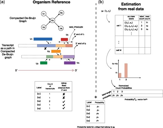
Overview of the minnow pipeline: On the right-hand side (a), the construction of unitig-based equivalence classes is depicted based on the compacted de Bruijn graph constructed from reference sequences. Unitigs u1 and u2 are discounted as they are more than MAX_FRAGLEN bp away from end of transcripts t1 and t2. Further the equivalence class is constructed as discussed in Section 2.1.3. On the right-hand side (b), the transcript-level equivalence class structure obtained from alevin is used to derive a per-gene probability vector. Finally, the probabilities are mapped directly to the unitig labels
Alternatively, instead of defining the label count probability vector for a gene globally over an entire experiment, minnow also supports defining cluster-local probability vectors when such information is given. Specifically, instead of normalizing over all cells, we normalize over all cells within a cluster (e.g. predicted cell type), deriving a probability vector , for each expressed gene gi in a cluster . This allows accounting for the fact that, due to changes in the underlying transcript expression that vary between clusters, the probability of observing (and hence generating) gene-ambiguous fragments may also change.
2.1.4 Assigning probabilities to
Qualitatively, represents the probability of sampling unitig u from gene gi to be equal to the empirically observed probability of equivalence classes containing gi that share u’s label count li. When provided, the cluster specific information can also be used here to derive an analogous function based on the cluster specific gene-level probability vector .
Both and fi, when used in conjunction with each other, give minnow the ability to sample the reads from references in a realistic manner. Given a gene g with count x, the selection process of candidate transcripts and underlying unitigs is as follows. Minnow first selects the set of unitigs that are part of the candidate transcripts. When there are multiple unitigs that can be potentially used, minnow initializes a multinomial distribution with parameters according to fg, where the random variable is the unitig to be selected next. Under this distribution, after x such random draws, x unitigs are selected (with replacement). For each such unitig, minnow randomly assigns the unitig to a corresponding transcript within that gene by scanning . In this composite selection process, while and determine the possible reference interval from which to sample, fi determines the probability of such sampling and, finally, dictates the sample size.
2.2 Generating RNA-seq sequences
2.2.1 Generation of cell barcodes and UMIs
Generating reads that match empirical degrees of gene-level ambiguity is one part of realistic single-cell RNA-seq data generation. Another main component is the generation of CB and UMI sequences, properly affected by amplification and sequencing errors. In minnow we concentrated on mimicking the process as it occurs in 10× data, though the modular nature of the tool makes designing modules for other droplet-based protocols straightforward. The length of the CB and UMI sequences can be provided by the user, by default we follow 10× v2 protocol for generating the CB and UMI sequences. Given the number of unique molecules (present in the experiment) provided in terms of the gene-count matrix, and the randomly generated UMI sequences, we perform a random assignment between UMIs and molecules. Once generated, a complete unit of sequence that undergoes PCR consists of a concatenated string of CB, UMI and the corresponding reference molecule (i.e. transcript) as sampled from .
2.2.2 PCR amplification and imputing sequence error
Once the set unique molecules are prepared, we simulate amplifying the molecules through multiple PCR cycles to generate a realistic distribution of PCR duplicates. We follow the standard protocol for PCR simulation (Best et al., 2015; Orabi et al., 2018). The PCR model in minnow can be described as a set of unbalanced probabilistic binary trees. The stochasticity of the model is determined by the probability of capture efficiency peff that can be externally set (default peff = 0.98). At each cycle, with probability peff, molecules are chosen for duplication. In each duplication step, a nucleotide in the molecule is mutated with probability perror (default perror = 0.01). At the end of simulating the PCR cycles, minnow randomly samples an appropriate number of molecules from the (duplicated) pool of molecules. Apart from providing this simple model, minnow also allows an optional flag to mimic the empirically supported model of PCR [described as Model 6 in Best et al. (2015)], where the efficiency of individual molecules is allowed to vary and is sampled from a normal distribution (default values ), and subsequently all the duplicated molecules inherit the efficiency from their parent. This step is highly stochastic, and can be customized to simulate PCR amplification given the uneven distribution of capture efficiency for individual molecules. We have implemented several optimizations, described in Supplementary Section 2, to reduce the computational burden associated with simulating PCR sequence duplication.
2.2.3 Start position sampling
Given the set of sampled duplicated PCR-ed molecules, minnow simulated the sequencing process of actual reads. As discussed in Section 2.1.4, minnow utilizes the precise location of the unitig on the transcript from which the read is drawn. The unitig acts as a seed for sampling read sequences from the reference. Given a unitig u, with offset position p and length l on a transcript t, we resort to two different mechanisms for determining start position. If the user chooses to use the empirical distribution of fragment lengths, then we randomly sample a fragment from a closed interval where probability of each fragment length is dictated by , and slack variable is set with proportional to the . While it is highly recommended to use an empirically derived read start position distribution (which comes packaged with minnow), in absence of such quantity, minnow samples from a truncated normal distribution with and a user defined σ (default set to 10). The intuition behind using such a distribution is to simultaneously use the ambiguity information while avoiding sampling reads from the same exact region again and again. This variance in sampling is important, since fragmentation occurs after the majority of amplification in the protocols we are simulating, and so ‘duplicate’ reads (reads from the same pre-PCR molecule) will tend to arise from different positions. Moreover, this framework creates an option for user to tune the σ in order to move away from unitig dependent sampling. Upon selecting the sequence minnow can be instructed to impute sequencing error in the sampled sequence. Minnow can accept a variety of error model for substituting nucleotides, and follows the same format of error model as used in Frazee et al. (2015).
3 Results
3.1 Assessing quantification tools using minnow
As its output, minnow produces the true abundance matrix , along with the raw FASTQ files containing the simulated reads. This enables rigorous testing of different quantification tools such as Cell-Ranger (Zheng et al., 2017), UMI-tools (Smith et al., 2017), etc. Hence, it is important to validate if the simulated reads generated by minnow are able to reproduce some of the challenges faced by these tools while consuming experimental data. One such factor that contributes to the performance of these tools is the mechanism by which they deduplicate UMI sequences (Srivastava et al., 2019). We observe that when we stratify the genes with respect to their gene uniqueness, the divergence between different tools start to emerge. As a proof of concept, we have run the popular quantification tools Cell-Ranger (2.1.0 and 3.0.0) and UMI-tools on minnow-simulated data. The UMI-tools-based pipeline we used is a custom one, which uses STAR (Dobin et al., 2013) for alignment, UMI-tools (Smith et al., 2017) for UMI resolution and featureCounts (Liao et al., 2014) for deduplicated UMI counting—we refer to this as the naïve pipeline.
The estimated abundances are correlated (Spearman and Pearson) with the true gene count provided by minnow. We note that number of cells detected by a downstream tool varies from what is initially present in the raw FASTQ files. Therefore, while calculating a cell specific local correlations, we consider only the subset of the cells that are predicted by all tools.
Minnow accepts a host of different input parameters, such as PCR-related mutation error, sequencing error, predefined custom error model for substitution, UMI pool size, number of PCR cycles, etc. As Cell-Ranger takes considerable time to finish (4–6 h for 4000 cells), we have limited ourselves to one run of 4 K cells of all tools, demonstrating the variance of different tools in the data. We observe that minnow scales efficiently with increasing numbers of cells. That is, the bottleneck in our assessments was the time required by the quantification tools, as minnow can simulate millions of reads in a few minutes. Thus, for demonstrating other effects (e.g. how the choice of different degrees of sequence ambiguity in mapping Splatter-generated counts to specific genes affects quantification accuracy), we have limited our assessment to smaller simulated datasets consisting of 100 cells each. An assessment of the computational performance of minnow is provided in Table 2.
3.2 Datasets
We have used two different datasets for benchmarking. For a global analysis, in terms of downstream quantification accuracy, we have used the publicly available peripheral blood mononuclear cells dataset, referred to as pbmc 4k dataset (Zheng et al., 2017), obtained from the 10× website. As discussed in Section 2.1, we first used alevin to estimate the gene-count matrix and the relevant auxiliary parameters, such as the equivalence classes. The gene-count matrix along with the auxiliary files are then used as an input to minnow. Minnow is run with two different configurations. First, we consider the ‘basic’ configuration, where no information other than the gene-count matrix from alevin is used. In the other configuration, referred to as ‘realistic’, we have made use of the equivalence classes produced by alevin, in addition to the compacted de Bruijn graph built on the transcript by TwoPaCo. The ‘realistic’ configuration also used the empirical fragment length distribution. In both the cases, we have used normal mode for PCR with fixed capture efficiency.
The other datasets we used are generated by Splatter (Zappia et al., 2017). Splatter accepts multiple parameters as input, including the generative model to use, the number of cells, the number of genes to express, etc. We used the splat model from Splatter to generate the gene-count matrix with default parameters. To manage the time consuming tools (Cell-Ranger-2 and 3), the analysis is restricted to 100 cells and 50 000 genes.
3.3 The presence of gene-level ambiguity drives the difficulty of UMI resolution and shapes the accuracy of downstream tools
With moderate numbers of fragments being sequenced per-cell and realistic diversity in the UMIs available to tag the initial molecules, existing pipelines appear to do a reasonable job of estimating the number of distinct molecules sampled from each gene within a cell. Yet, one major factor that appears to affect the accuracy of these different approaches is the level of sequence (specifically gene-level) ambiguity present in the simulated data. This is not particularly surprising, as neither Cell-Ranger (either version) nor the naïve pipeline are capable of appropriately handling such situations (i.e. to where should an UMI be assigned if its corresponding read maps equally well between multiple genes?). However, understanding this effect seems important, as the degree of gene-ambiguous reads in a typical scRNA-seq ranges from of the total reads (Srivastava et al., 2019).
To study the effect of gene-level ambiguity on quantification pipelines, we have stratified the global correlation plot with respect to the uniqueness score of a gene. The uniqueness score is specified by the ratio of two quantities: number of k-mers unique to a gene (i.e. only appearing within transcripts of this gene) to the total number of distinct k-mers present in the gene. According to this metric, the most-unique gene will have a score of 1 and the least a score of 0. The stratified plots (Figs 2 and 3) demonstrates that in the ‘basic’ simulation, the performance of all three tools are globally high. Interestingly, we note that Cell-Ranger-3 does slightly better than Cell-Ranger-2 (which in turn performs better than the naïve pipeline) for non-unique genes, despite the fact that it does not have a specific mechanism for resolving such cases. On the other hand, in the ‘realistic’ simulation, where gene-level sequence ambiguity was sampled to match the degree observed in even the most unique experimental data (this dataset exhibits gene-level multimapping meaning over 10% sequencing reads map to multiple genomic loci), the global performance decreased. One possible interpretation of such a considerable performance gap between different tools can be the specific method each method uses to categorize alignments [though all pipelines use STAR (Dobin et al., 2013) as their aligner], as well as differences in the algorithms they use to resolve UMIs. It is clear, however, that failing to resolve the multimapped reads can have a detrimental effect the accuracy of all of the quantification pipelines. The performance gap is magnified when we increase the fraction of reads sampled from less-unique gene sequences. Thus, it should be noted that failing to model empirically observed levels of sequence ambiguity can result in the simulation of unrealistic sequenced fragments, that fail to capture important characteristics of real data, and where the variability of different tools are hard to spot. Thus, to create more realistic and representative simulated data, it appears to be important to carefully match the degree of gene-level multimapping observed in experimental data.
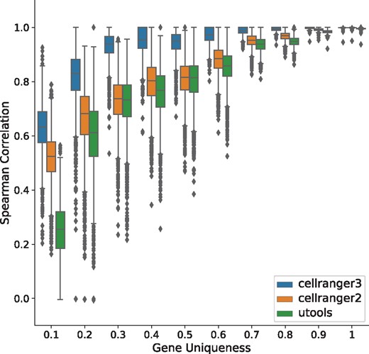
Performance of quantification tools, stratified by gene uniqueness, under a ‘basic’ configuration (based on pbmc 4k dataset)
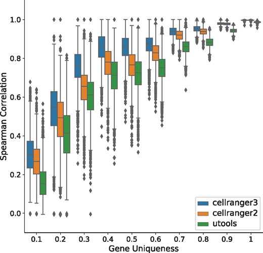
Performance of quantification tools, stratified by gene uniqueness, under a ‘realistic’ configuration (based on pbmc 4k dataset).
In the Splatter-based simulations, we have explored the performance of quantification pipelines on data representing a spectrum of degrees of sequence-level ambiguity. Splatter uses generative models to produce the gene-count matrix. Therefore, while the distributional characteristics of the simulated counts are designed to accord with experimental data, there is no specific relationship between the generated counts and specific gene present in an organism. While this presents a challenge—different mappings of simulated counts to different genes will result in different quantification performance—it also presents a degree of freedom to explore how the performance of tools changes as we hold the counts fixed, but alter the mappings between counts and specific genes. We use this freedom to model extreme situations, and to explore the sensitivity of different quantification pipelines as we alter how counts are mapped to specific genes. Specifically, we considered three different scenarios. First, we use the gene uniqueness scores defined above to sort the set of genes in increasing order (from least to most unique). Then, we assign the gene with lowest uniqueness score to the highest expressed gene label (aggregated over all cells) from the Splatter-obtained matrix and so on. This biased allocation purposefully increases the challenge of resolution for downstream tools. We call this configuration ‘adversarial’. In the second configuration, we have selected a random set of genes and followed the ‘realistic’ configuration by using the reference-based compacted de Bruijn graph and learned gene-level ambiguity distribution (as discussed in Section 2.1.2), following the same convention. We call this simulation ‘realistic’. Finally, the third configuration repeats the process of ‘adversarial’ but in reverse order, i.e. assigning the most-unique gene to the most abundant gene label. This final configuration is a situation where we expect to see minimum level of ambiguously mapped reads, thereby making the quantification challenge relatively easy for all downstream tools. We call this configuration ‘favorable’.
Table 1 shows the global correlation between three tools for all the above scenarios. We have also plotted (see Supplementary Fig. S1) the distribution of these metrics for all 100 cells in the simulation, to show the shift in global mean in both spearman correlation and mean absolute relative differences (MARD). In Supplementary Figure S1, we observe that for the ‘adversarial’ data, the performance of all pipelines is considerably depressed. Conversely, for the ‘favorable’ dataset (bottom row), the performance of all pipelines is considerably improved—and the gap between the different versions of Cell-Ranger and the naïve pipeline is reduced. The ‘realistic’ simulation falls nicely between these two extremes, suggesting that, while not as pronounced as one observes in the ‘adversarial’ scenario, the discarding of gene-ambiguous reads can have a considerable effect on quantification accuracy, even under realistic degrees of gene-level sequence ambiguity.
Spearman correlation and MARD are calculated with respect to ground truth under three different configurations based on the same gene-count matrix produced by Splatter
| Configuration | Correlation (Spearman) | MARD | ||||
|---|---|---|---|---|---|---|
| CR2 | CR3 | naïve | CR2 | CR3 | naïve | |
| Adversarial | 0.811 | 0.809 | 0.723 | 0.075 | 0.076 | 0.107 |
| Realistic | 0.920 | 0.915 | 0.880 | 0.043 | 0.046 | 0.076 |
| Favorable | 0.957 | 0.952 | 0.936 | 0.031 | 0.035 | 0.047 |
Note: CR2 and CR3 stand for Cell-Ranger-2 and Cell-Ranger-3, respectively.
3.3.1 Minnow maintains global structure in the simulated data
To compare the internal structure of the minnow generated data, we have compared the data matrices that are given to and produced by minnow. As shown in Supplementary Figures S2 and S3, we can see the number of clusters remains the same while some of the clusters are perturbed. This indicates that the minnow produced data can be effectively used for cell type specific analysis. Additionally, we have calculated variation of information (VI) (Meilă, 2007) as a metric to measure the distances between the clusters obtained by running Seurat’s clustering (Butler et al., 2018) algorithm on the count matrices produced by different methods, with respect to the clustering produced on the true count matrix, as output by minnow. The VI distances are 0.589, 0.613 and 0.632 for clusterings on the matrices produced by Cell-Ranger-3, Cell-Ranger-2 and naïve, respectively. While all of the tools do reasonably well, as expected, Cell-Ranger-3-derived clusters are closer to the truth than the other methods. The t-SNE plots shown in Supplementary Section 4 are plotted with the same seed after processing with Seurat.
3.3.2 Speed and memory of simulated sequence generation
The execution of minnow proceeds in two phases. First, it loads the gene-count matrix (as either a compressed binary or plain-text file) in a single thread. Then, it spawns multiple parallel threads (as many as specified by the user) to simulate reads deriving from different cells. This mechanism enables the most computationally intensive process (simulating PCR and generating read sequences) to happen independently and in parallel for each cell. This enables minnow to scale well with the number of threads when writing millions of reads to the disc. In Table 2, we have varied a number of parameters to test the computational requirements of minnow for generating simulated datasets of various sizes. Namely, we have varied the number of PCR cycles, the total number of cells simulated and number of threads used. The total wall clock time and peak resident memory reported using /usr/bin/time. We have limited the highest number of reads (default is 100 000) to be sampled and written to FASTQ file by minnow for each cell. This results in the approximate number of reads shown in the first column of Table 2. It should be noted that experiments containing more than cells are often generated from two or more separate experiments, concatenating the resulting count matrices after analyzing the samples in an independent manner. This can be achieved by running multiple instances of minnow. The performance is such cases would scale in a linear fashion as expected.
Timing and memory required by minnow to simulate data with various parameters
| Reads | Cells | PCR cycles | Threads | Time (hh: mm: ss) | mem. (KB) |
|---|---|---|---|---|---|
| 100M | 1000 | 4 | 8 | 0: 10: 44 | 7 556 108 |
| 100M | 1000 | 4 | 16 | 0: 5: 39 | 11 163 216 |
| 100M | 1000 | 7 | 8 | 0: 16: 56 | 8 723 320 |
| 100M | 1000 | 7 | 16 | 0: 9: 01 | 13 449 888 |
| 800M | 8000 | 4 | 8 | 0: 56: 28 | 28 249 676 |
| 800M | 8000 | 4 | 16 | 0: 31: 18 | 31 855 624 |
| 800M | 8000 | 7 | 8 | 1: 43: 32 | 29 246 148 |
| 800M | 8000 | 7 | 16 | 0: 53: 15 | 34 217 500 |
Simulated reads were generated on a server running ubuntu 16.10 with an Intel(R) Xeon(R) CPU (E5-2699 v4 @2.20 GHz with 44 cores), 512 GB RAM and a 4 TB TOSHIBA MG03ACA4 ATA HDD.
4 Conclusion
Single-cell sequencing has enabled scientists to gain a better understanding of complex and dynamic biological systems, and single-cell RNA-seq has been one of the pioneering biotechnologies in the field. Droplet-based assays, in particular, have proven very useful because of their high-throughput and ability to assay many cells. Driven by these exciting biotechnology developments, hosts of different methods have been developed in a relatively small time-frame to analyze the gene-by-cell count matrices that result from the initial quantification of these single-cell assay. Previously, various models have been proposed for simulating realistic count matrices (Zappia et al., 2017). These approaches implicitly assume that, apart from some fundamental limitations due to the biotechnology (e.g. cell capture, molecule sampling from small finite populations, etc.), the problem of ascertaining accurate gene counts from raw sequencing data by aligning reads and deduplicating UMIs is essentially solved. Consequently, the effect of the failures of these quantification pipelines to produce accurate gene expression estimates is not accounted for in the assessment of downstream analysis methods using this simulated data.
In this paper, we introduced minnow, which covers an important gap in existing methods for single-cell RNA-seq simulation (Westoby et al., 2018)—the read-level simulation of sequencing data for droplet-based scRNA-seq assays. We demonstrate the use of minnow to assess the accuracy of the single-cell quantification methods under different configurations of sequence-level characteristics, ranging from adversarial, to realistic, to favorable. We propose a framework for the simulation of synthetic dscRNA-seq data, which simulates the CB, UMI and read sequences, while accounting for the considerable effects of PCR and realistic sequence ambiguity in generated reads. Further as a flexible framework minnow can be easily used to create a variety of possible configurations, such as changing fragment length distribution, sequencing error, collision rate, etc., to do robust testing of computational tools. We believe minnow will help the community to develop the next generation of quantification tools for droplet-based scRNA-seq data. It provides the first comprehensive framework to simulate such data at the sequence level, allowing users to validate the accuracy of different methods and providing useful feedback to determine future directions for improving quantification algorithms. Minnow is an open-source tool, developed in C++14, and is licensed under a BSD license. It is available at https://github.com/COMBINE-lab/minnow.
Acknowledgements
We would like to thank Charlotte Soneson for insightful conversations and for providing valuable feedback during the creation of minnow.
Funding
This work was supported by NSF award CCF-1750472 and by grant 2018-182752 from the Chan Zuckerberg Initiative DAF, an advised fund of Silicon Valley Community Foundation. The authors thank Stony Brook Research Computing and Cyberinfrastructure and the Institute for Advanced Computational Science at Stony Brook University for access to the SeaWulf computing system, which was made possible by NSF grant 1531492.
Conflict of Interest: R.P. is a co-founder of Ocean Genomics. H.S. and A.S. declare no conflicts.
References

