


Abstract
De novo transcriptome analysis using RNA-seq offers a promising means to study gene expression in non-model organisms. Yet, the difficulty of transcriptome assembly means that the contigs provided by the assembler often represent a fractured and incomplete view of the transcriptome, complicating downstream analysis. We introduce Grouper, a new method for clustering contigs from de novo assemblies that are likely to belong to the same transcripts and genes; these groups can subsequently be analyzed more robustly. When provided with access to the genome of a related organism, Grouper can transfer annotations to the de novo assembly, further improving the clustering.
On de novo assemblies from four different species, we show that Grouper is able to accurately cluster a larger number of contigs than the existing state-of-the-art method. The Grouper pipeline is able to map greater than 10% more reads against the contigs, leading to accurate downstream differential expression analyses. The labeling module, in the presence of a closely related annotated genome, can efficiently transfer annotations to the contigs and use this information to further improve clustering. Overall, Grouper provides a complete and efficient pipeline for processing de novo transcriptomic assemblies.
The Grouper software is freely available at https://github.com/COMBINE-lab/grouper under the 2-clause BSD license.
Supplementary data are available at Bioinformatics online.
1 Introduction
Advances in sequencing technologies have allowed the efficient and accurate exploration of transcriptomes beyond the scope of genetic model organisms (Ekblom and Galindo, 2011; Marioni et al., 2008). Transcriptome sequencing opens the door to understanding gene expression even in species with no high-quality reference genome, which constitutes a vast majority of known species (Martin and Wang, 2011). Some common uses of transcriptome sequencing include variant detection, fusion and alternative splicing event discovery, and differential expression analysis (Soumana et al., 2015; Stubben et al., 2014). In organisms where the transcript sequences are not known a priori, a crucial initial step is assembling the transcriptome using short sequencing reads. In short read sequencing, a transcriptome is typically sequenced to high depth, resulting in tens to hundreds of millions of reads, which then need to be assembled to reconstruct the original transcript sequences; a process called de novo assembly. These transcripts will later act as the ‘reference’ for subsequent analyses. For instance, in a differential analysis pipeline, the reads are first mapped back to the assembled transcripts to infer transcript abundance (Li and Dewey, 2011).
There are many popular tools for assembling the full-length transcripts from short reads by leveraging the redundancies and overlap between reads, such as Trinity (Haas et al., 2013), Oasis (Schulz et al., 2012) and Trans-ABySS (Robertson et al., 2010). Similarly, there are tools that can be used to improve the quality of the assemblies generated by these methods (Cabau et al., 2017; Durai and Schulz, 2016). However, despite the powerful algorithms and heuristics adopted, the final output sequences (i.e. contigs) often don’t represent the full-length transcripts. In other words, many transcripts are fragmented into a set of non-overlapping contigs. This results from numerous difficulties in assembly including (but not limited to) errors in the sequenced reads, transcriptome complexity arising from alternative splicing and paralogous genes, uneven or insufficient coverage across the length of the sequences molecules, and deficiencies in the underlying approaches used for assembly (e.g. places where the computational problem being solved does not match well with the underlying biology). All of these can lead to a collection of output contigs, which is much larger than the actual set of transcripts assayed.
Because of the potentially low quality of de novo assembly output, it is more promising and robust to pursue gene-level differential expression analysis instead of transcript-level (i.e. contig-level) analysis. To obtain gene-level information, we need to infer the contigs that represent parts of the same transcript and those that represent isoforms of the same gene, and group them together. This is what methodologies such as those by Davidson and Oshlack (2014), Ptitsyn et al. (2015) and Srivastava et al. (2016) propose. Corset computes a hierarchical clustering based on the shared counts of the contigs, and RapClust clusters a sparse graph, called the mapping ambiguity graph, with nodes representing the contigs, and edges weighted based on the abundances of the contigs sharing common reads. Moreover, for meaningful interpretation of these clusters and various analyses, it is important to have some notion of what the contigs in the de novo assembly represent (Garber et al., 2011). Often, we have annotated genomes or transcriptomes from species closely related to the non-model organism under study. This information can be exploited to accurately annotate the contigs of a de novo assembly and improve our understanding of the function of the genes that demonstrate differential expression. Traditionally, variants of BLAST (Altschul et al., 1990) are used to perform this annotation and then complete Gene Ontology (GO) analysis (Ji et al., 2012; Parchman et al., 2010).
Currently, several methods exist to process de novo assemblies in order to improve downstream analyses and ease the interpretation of results from such analyses. However, each method has its limitations, and apart from Corset, there doesn’t exist a tool that provides a complete pipeline for clustering and annotating de novo contigs. We introduce Grouper that subsumes and improves on the framework of RapClust and can be used for accurate and efficient processing of de novo transcriptome assemblies, to yield clusters of contigs and transfer labels to them from an annotated genome in a matter of tens of minutes. The underlying algorithms in Grouper transfer information from de novo assemblies onto a graph, suggesting a useful future direction for de novo transcriptome analysis beyond direct sequence analysis of the assembled contigs. The complete Grouper pipeline also provides quantification information that can be used for differential expression analyses. The Grouper software is freely available at https://github.com/COMBINE-lab/grouper.
2 Materials and methods
2.1 Overview
The first step for the analysis of RNA-seq data, in the absence of a reference genome, is generating a de novo transcriptome assembly, using tools such as Trinity (Grabherr et al., 2011) and Oases (Schulz et al., 2012). The assemblies tend to have a large number of fractured or incomplete contigs that do not represent full-length transcripts. Grouper aims to cluster these contigs such that, under ideal conditions, each cluster represents a single gene with its various transcripts. To do so, the original RNA-seq reads are mapped to the assembly using Salmon, which generates quantification estimates and fragment equivalence classes. Each equivalence class contains fragments that are mapped to the same set of contigs from the de novo assembly, hence encoding the multi-mapping structure of sequencing reads in relation to a reference. These are processed by Grouper to construct a mapping ambiguity graph, where the nodes are the set of contigs and are connected by edges based on the reads that multi-map between them. This graph is then further improved using quantification estimates and, optionally, orphan read information from Salmon. Annotations can also be added to the graph from the annotated genomes of closely related species using Grouper’s labeling module. The final graph is then clustered providing groups of contigs as the output and annotations (if added). Downstream analyses can then be done treating these groups as putative genes. For example using the R tool, tximport (Love et al., 2017), to aggregate abundance estimates to the cluster level, which can then be used for differential expression testing. This complete pipeline is illustrated in Figure 1.
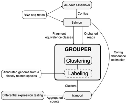
Grouper pipeline: Grouper consists of two modules with different modules, Clustering and Labeling. The goal of Clustering is to put contigs from a de novo assembly into groups that represent individual genes. The labeling module assigns a label to each of these clusters using annotated genomes from closely related species. Hence, the labeling step is optional. Grouper needs equivalence classes as input, which can be generated using Salmon on the raw RNA-seq reads. Orphan reads are optionally used in the Clustering module. The output of Grouper are clusters representing a putative contig-to-gene mapping, which may be labeled using an annotated genome from a related species. Quantification estimates can then be summed to the cluster level for downstream differential expression analyses using tximport
There are two main modules in Grouper: clustering and labeling. The former takes as input the output from Salmon (Patro et al., 2017), where RNA-seq reads are mapped against a de novo assembly and quantified. This is used to generate the mapping ambiguity graph and then cluster the unannotated contigs. Clustering module is the main module of Grouper, and the labeling module is built on top of this framework. It is optional and requires an additional input of annotations from species closely related to the one used for assembly. Both of these modules help improve and annotate the assembled contigs for downstream analyses.
2.2 Clustering
The clustering module (Supplementary Fig. S1) builds on the work in RapClust, a tool for accurate and fast clustering of contigs from de novo assemblies (Srivastava et al., 2016). The original work makes use of the intrinsic sequence similarity within the contigs, expressed in the form of equivalence classes, and the transcript-level expression estimates. The clustering module consists of multiple steps, the first being the construction of the mapping ambiguity graph using equivalence classes, generated by Salmon during the mapping and quantification phase. The graph, G, is a weighted, undirected graph with contigs (having at least 10 reads mapped to them) as its vertices. Two vertices are connected by an edge if they share multi-mapping reads, meaning that a read is mapped to both of the contigs. The edge weight is indicative of the amount of similarity between the two contigs, and, as with the weighting function used in Corset (Davidson and Oshlack, 2014), is defined based on the number of reads that these contigs share compared to the number of reads that map to each of them individually. Once the graph is constructed, an additional filter accounts for contigs from paralogous genes by removing edges that connect contigs with read counts that vary significantly. Optionally, this graph can be further improved using two steps. The first involves adding edges using orphan reads (as output by Salmon), where the ends of a paired-end read map to two different contigs, with similar expression estimates. In the second step, instead of simply removing adjacent contigs with significantly varying read counts, we compute a min-cut separating the two components containing these contigs, forcing them to reside in distinct clusters in the final output. Once the mapping ambiguity graph has been updated, it is clustered using MCL (Dongen, 2000), an off-the-shelf graph clustering method, to obtain groups representing a mapping of contigs to genes.
2.2.1 Equivalence classes
Grouper uses the idea of fragment equivalence classes to estimate similarity between two fragments or contigs. Similar notions of equivalence classes have previously been defined and used for multiple purposes (Nicolae et al., 2011; Patro et al., 2017; Salzman et al., 2011; Turro et al., 2011). We define an equivalence class over a set of fragments on the basis of the transcripts to which the fragments map. Fragments fi and fj belong to the same equivalence class if , where is the set of transcripts to which fragment fi maps, and is the set of transcripts to which fj maps. Each equivalence class also has an associated count that is simply the number of equivalent fragments it contains.
2.2.2 Graph construction
2.2.3 Filtering
After constructing the mapping ambiguity graph, we apply two main filters, adopted from Corset (Davidson and Oshlack, 2014), before clustering it. In the first step, we remove a node and all its connections from the graph if the total number of reads mapping to the representative contig in all the samples is fewer than 10. This reduces the noise in the graph since, based on the number of mapping reads, such a node will have highly weighted edges connecting it to neighbor nodes but is probably a short or misassembled contig. The second filtering step uses quantification information provided by Salmon to reduce the number of edges between contigs that have a similar sequence but significantly varying expression estimates across conditions and are, therefore, unlikely to be from the same underlying gene. This filter helps remove contigs that likely originated from paralogous genes and cannot be separated based only on the sequence. Specifically, the filter performs a likelihood ratio test, where the likelihood values are calculated as detailed in Equations S1, S2 and edges with value are removed from the graph.
2.2.4 Orphan reads
The first optional filter in Grouper adds edges to the mapping ambiguity graph using information from orphan reads. In a paired-end sequencing run, the output is a series of reads such that each pair of reads is sequenced from a single fragment that originated from the same transcript. Hence, these reads should ideally map to a single contig in the assembly. However, there are cases where one end of the read is mapped to one contig and the other end to a different contig. We call such reads as orphans, as their parent contig is not unique or identifiable. These can occur due to two main reasons. The first is (adversarial) sequencing error, which makes it impossible to correctly identify the original source of the read. The second is misassembled or broken contigs, which are a common artifact of the de novo assembly procedure. Since orphan reads provide extra information about which contigs hypothetically originate from the same transcript, we use these reads to join contigs in the underlying mapping ambiguity graph by adding an edge between the two contigs in if they share a pair of orphan reads between them. The edge is only added if the absolute value of the ratio of the expression (TPMs) of the two contigs, calculated by Salmon, is less than 2. This reduces the number of false positives in the clustering method, since orphan reads can be caused by errors in the sequencing methodology, or could falsely join together two contigs from distinct transcripts or related genes. Adding an edge in this way helps improve the recall of Grouper over other methods.
2.2.5 Min-cut filter
The second optional filter uses the likelihood ratio test based on the quantification information, as explained above, but instead of simply removing the edge between the contigs, a min-cut is performed on the graph to completely separate the two contigs into disjoint subsets of the graph. This ensures that in the final graph clustering step, the two contigs are not put into the same cluster based on a longer path joining them. Based on the de novo assembly, this min-cut can improve the accuracy of downstream differential expression tests. However, depending on the complexity of the underlying graph structure, this can take a long time to run and is therefore optional. (We note that we have not attempted to optimize the algorithm used to perform the min-cut, and that it is likely that this process can be made considerably faster.)
2.3 Labeling
The labeling module (Supplementary Fig. S2) is best considered as a method capable of ‘boosting’ an initial set of annotations by accounting for expression and sequence similarities within the de novo assembly rather than being a complete annotation pipeline. Graph-based methods have previously been used to transfer information in biological data as well (Libbrecht et al., 2015). Furthermore, this module not only boosts annotation quality, but also uses these annotations to improve contig-level clustering, which can lead to more accurate differential analysis results. We begin by labeling nodes of the mapping ambiguity graph, G. This is done by mapping the annotations from a closely related species to the contigs in the de novo assembly, using a traditional approach, such as a BLAST search (Altschul et al., 1990). Subsequently, a graph-based semi-supervised learning method for label propagation is used to transfer these initial annotations to unannotated nodes in the graph. For this purpose, we use the adsorption algorithm, which relies on random walks through the graph and has been used to efficiently propagate information through a variety of graphs in its various applications (Baluja et al., 2008). On top of this label propagation, we build an iterative algorithm to modify the topology and edge weights in the graph based on the current labeling. This process is repeated until the topology of the graph converges. The final result of our approach is a collection of annotations for the contigs in the de novo assembly and a graph that best represents the relationship between these contigs based on the available sequence and annotation information, which can then be clustered, as before, using MCL.
2.3.1 Initial annotation
The initial labeling can be passed to this step in two formats. Take A to be the set of contigs from the de novo assembly, and B the set of annotated transcripts from the related species. The first is a simple mapping from A to B. The second format consists of two separate files where the first file contains results from a nucleotide BLAST of the de novo assembly of the test species against the database constructed using the annotated reference from the related species and vice-versa in the second file. Hence, the first file contains a mapping from A to B and the second from B to A. In the latter case, the two BLAST files are sorted using the bit score, with ties being broken by the e-value and contigs are given their corresponding consensus label, with a probability value proportional to the length of overlap between the sequences. The contig is not labeled if no consensus exists, i.e. if the best hit in A → B is not the same as the best hit in B → A. This labeling and the mapping ambiguity graph are passed to the labeling module and it proceeds executing, iteratively, the steps of its algorithm. In the description of the algorithm, we use the following notation:
is the mapping ambiguity graph at the iteration
Et is the edge set at the iteration
is an edge from Et and is an un-ordered pair
2.3.2 Edge manipulation
After labeling contigs, edges in the graph are changed, iteratively, in two ways based on the shared labels and edge weights from the prior iterations of the algorithm:
Let t + 1 denote the current iteration of the algorithm, and let be an edge in the set Et of edges. The weight of e, denoted as , can be updated if there are labels common between two contigs sharing an edge and is calculated as . Here, α is set to 0.8 for our tests, is the original edge weight in the input graph (i.e. G0) and p1, p2 are probabilities of each contig having a label l from the set of shared labels, L. We chose a value for α based on the species we tested against and show that depending on the proximity of the annotated species to the test species, the effect of this value varies. For species that are more distantly related to the test species, smaller values of α give better results, since the labels obtained using sequences may not be accurate but are initialized with a probability of 1.0 by default, unless the user specifies other values as input.
New edges are added to the graph in cases where two contigs share a label with high probability, but do not have an edge between them. The new edge weight is calculated in the same way as above. However, instead of the original edge weight (since no edge originally existed), we instead use the median of the edge weights connecting the two vertices to their neighbors in the graph. The edge is only added if the joint probability of shared labels is greater than 0.9. This threshold is chosen to avoid adding a large number of false edges, especially in the first iteration when a majority of labels are likely assigned a probability of 1.0.
2.3.3 Label propagation
Using results from BLAST, a portion of the contigs in the mapping ambiguity graph are labeled. The graph-based, semi-supervised learning algorithm, adsorption (Baluja et al., 2008) [we use the implementation from the Junto library (Talukdar and Pereira, 2010)], is used to extend these labels to contigs that have a large number of overlapping mapped reads and, therefore, an edge between them in the graph. The algorithm works by taking random walks through the graph carrying label information. This information is propagated based on three probabilities associated with each node: pinj, the probability of stopping the current random walk and emitting a new label, pabnd, the probability of completely abandoning the walk and pcont, the probability of continuing the random walk with the current label.
We do not run the label propagation algorithm until convergence, since we wish to utilize information at each iteration to update the graph and change the edges. Due to this, labels from the current node are only propagated to all highly connected neighbors, reducing the number of false positives as well. At the end of label propagation, each label associated with a contig has a weight in the range , and each contig may have up to a maximum of three labels (a limitation of the implementation of the adsorption algorithm we adopt). Once the topology of the graph converges, we cluster it as before. The convergence criteria we set in this case is that the number of edges added in the current iteration is less than or equal to 5% of those added in the previous iteration. The final iteration step also outputs a partial mapping from contigs in the de novo assembly to transcripts or genes in the related annotated species. Hence, the clusters represent a putative contig-to-gene level mapping and each cluster can be assigned a gene label based on the label for the majority of contigs in the cluster.
3 Results
3.1 Test setup
To analyze the performance of different modules in Grouper, we ran the tool on datasets from four different organisms, varying in complexity and genome size. We consider datasets from human, mouse and yeast. To check for the effect of assembly quality, we tested our tool assemblies generated using Trinity (Grabherr et al., 2011) as well as with the reference transcriptomes of each organism (the latter experiments acting as an upper bound of how we expect the method might perform as the de novo assemblies become more accurate and complete). We also included a plant species, Asian rice, in the analysis to show the ability of Grouper to process data containing many transcripts with high sequence similarity. Over the four datasets, we compared the clusters produced by Grouper against those predicted by the contig clustering method, Corset (Davidson and Oshlack, 2014). All results include those from the original Grouper algorithm, as well as those with the optional filters applied. We shall refer to the base algorithm as Grouper, which is adapted from RapClust (Srivastava et al., 2016) and uses only the read counts to filter contigs and edges, Grouper (O) refers to the results of Grouper considering the orphan read pairs, and Grouper (O + M) refers to results after applying both the optional post-processing steps, adding edges using orphan reads and performing min-cuts on the graph using read counts. Details of the datasets and parameters used to run the tools are provided in the Supplementary Material.
3.2 Grouper increases the accuracy and speed of clustering
To calculate the accuracy of the clusters produced by different methods, we first mapped reads using Salmon (Patro et al., 2017) (for Grouper) and aligned reads using Bowtie (Langmead, 2010) (for Corset). This step was done with both the assemblies generated by Trinity and the annotated reference transcriptomes. Since the ‘true’ clusters in the former case were generated using BLAST (see Section 2), they are not guaranteed to be free of errors. To account for this, we ran the same tests on the reference transcriptomes, where the truth was obtained from the annotated genomes. This result suggests how these clustering methods may perform as the quality of the assemblies improves. In both cases, a true positive is counted if two contigs in the same cluster have the same ‘true’ gene label and a false positive if they do not. Conversely, a false negative is counted if two contigs that have the same label under the truth are put in separate groups by the clustering method.
The results from the de novo assemblies are shown in Figure 2a. Looking at the F1 scores, Grouper performs consistently better than Corset, particularly with the inclusion of the two additional filters. In general, Grouper clusters have higher recall but slightly lower precision than those predicted by Corset. Although the optional filters in Grouper do not make a large difference in the accuracy of the clusters, depending on the size of the dataset, we recommend using them since minor differences in the clusters can lead to varying differential expression calls. The total number of contigs clustered in each case does not vary significantly, as shown on the left panel in Supplementary Table S1, except in the case of the human dataset where Grouper clusters a much larger number of contigs. In our experiments, both Grouper and Corset were told to ignore contigs with fewer than 10 reads mapping to them (the default parameter in both tools). However, since both methods use different quantification pipelines, the overall percentage of reads mapped by Salmon is much higher, as shown in Table 1. Therefore, within the variants of Grouper, only a few extra contigs are included in the graph when considering counts from orphan reads.
Percentage of reads aligned by each method on the de novo assemblies and the reference transcriptomes
| De novo assemblies | Transcriptomes | |||
|---|---|---|---|---|
| Bowtie | Salmon | Bowtie | Salmon | |
| Human | 86.34 | 95.76 | 86.99 | 94.72 |
| Yeast | 66.48 | 97.84 | 56.47 | 87.99 |
| Mouse | 30.74 | 86.01 | 88.2 | 85.98 |
| Rice | 82.28 | 92.36 | 79.45 | 83.8 |
| De novo assemblies | Transcriptomes | |||
|---|---|---|---|---|
| Bowtie | Salmon | Bowtie | Salmon | |
| Human | 86.34 | 95.76 | 86.99 | 94.72 |
| Yeast | 66.48 | 97.84 | 56.47 | 87.99 |
| Mouse | 30.74 | 86.01 | 88.2 | 85.98 |
| Rice | 82.28 | 92.36 | 79.45 | 83.8 |
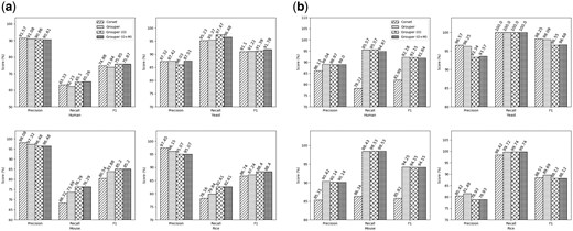
Accuracy results: The precision, recall and F1 scores using different clustering approaches on de novo assemblies (a) and reference transcriptomes (b) from the test species
To demonstrate the effect of transcriptome assembly methods on the accuracy of the clusters produced, we repeated the same tests on the original transcriptomes (results presented in Fig. 2b). In the case of human, mouse and rice, Grouper performs better than Corset in terms of both precision and recall. For the yeast dataset, Grouper performs slightly worse. However, it is important to notice that Grouper clusters 6725 contigs, whereas Corset clusters only 3592, as shown in the right panel of Supplementary Table S2. Hence, Grouper discards fewer reads (Table 1), and therefore contigs, while maintaining the accuracy of the resulting clusters. The better accuracy of clusters produced by Grouper, especially in the case of the human and mouse datasets, show that as transcriptome assembly methods improve, the Grouper algorithm may have the ability to perform significantly better than existing contig clustering tools. This, we believe, may also reduce the need for the additional filters.
The time, in seconds, taken for each clustering method is reported in Table 2 and the memory usage in Supplementary Table S3. On the de novo assemblies, all variants of Grouper are considerably faster than Corset, taking a few minutes at most to process the input data and generate clusters. This is also true for the tests using reference transcripomes, except in the case of human when both the optional filters are enabled. The large runtime on this dataset is due to the computational complexity of repeatedly performing min-cut on the large (and denser) mapping ambiguity graph. The results in Table 2 represents only the time needed for the clustering component of the tools. However, the complete pipeline also includes aligning reads against the input reference sequence. Corset takes as input an alignment BAM file, generated using Bowtie, whereas Grouper takes as input the equivalence classes generated by Salmon. We report times for running these two tools on the raw RNA-seq reads in Supplementary Table S4. Salmon is able to map and quantify reads within minutes, whereas Bowtie can take up to a few hours. Overall, the Salmon and Grouper pipeline takes only a few minutes to process the sequencing data and generate clusters.
Clustering time of each method using the de novo assemblies and the reference transcriptomes (in seconds)
| De novo assembly | Transcriptome | |||||||
|---|---|---|---|---|---|---|---|---|
| Corset | Grouper | Grouper (O) | Grouper (O+M) | Corset | Grouper | Grouper (O) | Grouper (O+M) | |
| Human | 902.19 | 50.49 | 100.93 | 269.99 | 24479.29 | 154.46 | 296.62 | 549160.99 |
| Yeast | 167.8 | 1.92 | 8.67 | 11.28 | 234.6 | 3.23 | 10.07 | 33.06 |
| Mouse | 348.91 | 14.31 | 46.12 | 46.12 | 503.54 | 27.65 | 52.65 | 52.65 |
| Rice | 234.96 | 37.02 | 74.85 | 74.85 | 259.93 | 12.11 | 24.95 | 24.95 |
3.3 Accuracy in detecting differentially expressed genes
Transcriptome assembly methods tend to produce incomplete or fractured contigs that eventually confound downstream differential expression tests. Hence, it is important that the clusters produced by processing the assembled contigs approximate the actual gene-level expression estimates. To test this, we perform differential expression analysis on the clusters generated by the different methods. Each cluster is given a gene label, which is obtained by taking the contig-to-gene mapping and labeling a cluster with the most frequently occurring gene label among its constituent contigs. Cluster-level expression estimates for Corset are provided as output by the tool itself, and for Grouper, are obtained using the R package, tximport (Love et al., 2017), to sum read counts provided by Salmon to the cluster level. Then, Limma Voom (Law et al., 2014) is used to obtain corrected P-values for the hypothesis that each cluster is differentially expressed, calling genes with corrected P-value less than or equal to 0.05 as differentially expressed. The same procedure, using counts from Salmon or RSEM (Li and Dewey, 2011), was repeated for the ‘true’ clustering to obtain ground truth.
We repeated this test on the human and yeast datasets, where we had RNA-seq samples under varying conditions. Note that the other datasets only include samples from a single condition, and therefore cannot be used for differential expression analysis. The results from this analysis are presented in Figure 3, and in Supplementary Figure S3. The curve represents the accuracy of the different methods. In the human dataset, the different variants of Grouper perform similarly to Corset, though they exhibit a slightly lower AUC. On the other hand, in the yeast dataset, Grouper variants perform considerably better than Corset, performing almost 1.25 times better when run with both the optional filters. This shows that Grouper consistently generates good clusters, not just in terms of the accuracy of the actual clustering, but also in terms of downstream analysis performed on them. Interestingly, this test also shows that the accuracy of the clustering itself is not immediately or proportionally reflected in differential gene expression testing accuracy (at least under the testing scheme used here).
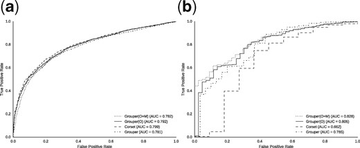
DGE results: The curve represents the accuracy (true positives against false positives) of calling differentially expressed genes using Salmon counts as ground truth, represented by the clusters generated by each method in the human (a) and yeast (b) datasets
3.4 Combining information from annotated transcriptomes
For a meaningful interpretation of differential expression analyses, there needs to be some notion of which genes are represented by the individual contigs. Often, we have annotated genomes from species that are closely related to the non-model organism assembled. Information from this annotation can be harvested to accurately annotate contigs from the de novo assembly. Traditionally, variants of BLAST are used to transfer these annotations. Corset also provides a method for transferring annotations by aligning reads against the annotated transcriptome and processing all the alignment files together. We provide a labeling module in Grouper that allows for efficiently transferring annotations to the de novo assembly and then propagating them through the mapping ambiguity graph to eventually annotate a larger number of contigs.
We compare our results against results from Corset, BLAST using all the contigs in the assembly, BLAST using only the contigs that have greater than 10 reads mapping to them, and Trinotate (Haas et al., 2013), using both nucleotide and protein level BLAST against the SwissProt database. Since there is no obvious and complete mapping between the contigs and annotations from the related species, we choose to compare the different methods based on their ability to give contigs from a single gene the same label and, in turn, cluster them together for down-stream analyses. We did the analysis using an annotated, closely related genome for the human, mouse, and Asian rice datasets. Annotated genomes used were from gibbon, ratand red rice, respectively. The results, presented in Figure 4, show that although precision of the clusters generated by the labeling module in Grouper is slightly lower than the next-best method, the gain in recall is significantly higher, resulting in clusters with higher overall F1 scores.
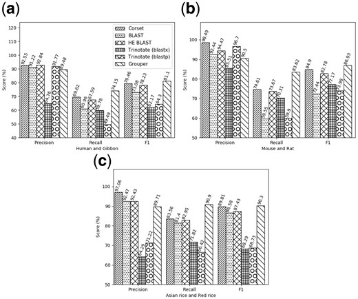
Accuracy results: The precision, recall and F1 scores from different annotations methods on the human genome using the gibbon as a closely related annotated species (a), on the mouse dataset using the rat genome (b), and the Asian rice dataset using the red rice genome (c). Note: HE BLAST refers to using BLAST to annotate only the contigs that have more than 10 reads mapping to them, as quantified by Salmon
In addition to being accurate, Grouper assigns annotations to a greater number of contigs than simply using BLAST. This is a benefit of the label propagation step which, in each iteration, makes use of the previous information to continue labeling connected components in the graph. This means that some of the previously unannotated contigs, which could not be annotated on the basis of sequence similarity alone, are labeled by the end of the iterative process. In this way, Grouper is able to assign annotations to 2325, 4957 and 3655 extra contigs in human, mouse and rice assemblies, respectively. The larger number of annotations could be helpful in down-stream analyses for specific genes. On the other hand, Corset does not directly label contigs in the de novo assembly but adds the annotated transcripts in clusters along with them. This cluster-level information can then be used to infer annotations, which adds to the complexity of the pipeline.
Along with producing more complete and accurate annotations, Grouper is also much faster than the other tools, as shown in Table 3. The time taken for Grouper includes the time to run Salmon (which generates contig-level abundance estimates), to generate equivalence classes, to construct the mapping ambiguity graph, to run BLAST to generate the initial contig labels and then to propagate the labels, alter the graph topology and cluster the contigs. Similarly, Corset timing includes time to align reads in each sample against the reference. Grouper takes 20 min in human, with a total of 23.2 million reads across six samples and 107 389 contigs in the de novo assembly. The other species take less than 15 min, with a total of 10.5 million reads and 75 727 contigs in mouse and 8 million reads and 99 745 contigs in rice. In comparison, the other tools take several hours to run on these datasets.
Total time (in minutes) for each pipeline used to annotate contigs in a de novo assembly
| Corset | Trinotate (nucl.) | Trinotate (prot.) | Grouper | |
|---|---|---|---|---|
| Human | 513.28 | 2356.13 | 781.56 | 20.85 |
| Mouse | 272.88 | 1616.01 | 498.3 | 10.23 |
| Rice | 208.79 | 983.37 | 424.02 | 11.19 |
| Corset | Trinotate (nucl.) | Trinotate (prot.) | Grouper | |
|---|---|---|---|---|
| Human | 513.28 | 2356.13 | 781.56 | 20.85 |
| Mouse | 272.88 | 1616.01 | 498.3 | 10.23 |
| Rice | 208.79 | 983.37 | 424.02 | 11.19 |
Note: Note that these results include alignment and quantification times, as well as the clustering time, for Grouper and Corset.
4 Discussion
The analysis of transcriptomic profiles via RNA-seq remains a challenge especially when the organism being assayed lacks a high-quality reference transcriptome. Considerable progress has been made in terms of both the sequencing technologies available (providing higher depth and higher quality read information) and the computational approaches used to reconstruct the underlying transcriptome from the output of these sequencing experiments. Yet, even the best available assembly approaches often yield incomplete (and sometimes incorrect) transcript sequences. The fractured nature of these assemblies complicates downstream analyses, such as differential expression analysis, and results in spurious false-positive calls, as well as a loss of statistical power in terms of genes that can truly be identified to be differentially expressed.
Following the general framework originally laid-out by Davidson and Oshlack (2014), we introduce Grouper, a tool for processing de novo transcriptomic data that groups together assembled contigs into putative genes based on evidence of shared sequence. These putative genes can then be more accurately and stably quantified. We cast this problem of determining transcript groups as one of clustering a mapping ambiguity graph, that we construct using multi-mapping read information. We introduce useful heuristics for both filtering this graph (to remove likely spurious edges), and for augmenting this graph with information obtained from orphan mappings that likely result from the incomplete nature of the underlying assembly. We demonstrate that this clustering problem can be solved efficiently and accurately, and that treating the resulting clusters as putative genes can lead to biologically meaningful analyses.
Simultaneously, we also introduce a novel, graph-based approach for annotating the transcripts in a de novo assembly using information from related organisms. Rather than relying only on the sequence similarity between the two references, we also make use of the mapping ambiguity graph that provides evidence of the sequence similarity of the contigs within the assembly. We initially label a subset of the contigs (nodes in the graph) with high-confidence labels transferred from a related organism. Then we take advantage of the graph structure by applying a semi-supervised label propagation algorithm (Talukdar and Pereira, 2010), to propagate gene labels among highly related contigs within the assembly. We demonstrate that, when labeling information from related organisms is included, the labeling scheme that relies on the graph-based label propagation approach moderately outperforms other approaches, measured by the quality of the resulting clusters (Fig. 4). Thus, we show that Grouper provides an accurate and efficient way to improve the quality of de novo transcriptome analysis by allowing the aggregation of contigs into biologically meaningful groups (putative genes), and that it can effectively make use of related transcriptomes when available. Given its relatively modest computational overhead, we believe that Grouper can become a popular tool to help tackle some of the difficult tasks faced in de novo transcriptome analysis.
While Grouper performs well in our tests, and is able to cluster and annotate contigs from de novo assemblies efficiently, there is clearly a limit to the accuracy it can obtain based on the quality and completeness of the underlying de novo assembly. This is demonstrated in Figure 2, where we see considerably improved performance of Grouper (and Corset) when they are provided with the reference assemblies as input. The results of this analysis suggest that a major limiting factor in improving performance is actually the quality of the de novo assemblies being produced. While de novo transcriptome assembly is known to be a very challenging problem, progress is nonetheless being made both in terms of the computational approaches being developed and in terms of the biotechnologies being brought to bear on the problem. In the future, we are interested in incorporating into Grouper the evidence that can be provided by long read transcriptome sequencing (e.g. by PacBio Iso-Seq or nanopore’s direct RNA-sequencing technology). While these technologies often do not obtain the same depth of coverage as traditional RNA-seq, and therefore are less likely to sequence rare isoforms, they nonetheless provide high-quality structural information about the expressed transcripts, and we anticipate that such data will be able to provide information about the ‘backbone’ gene structure by which shorter contigs can be grouped. As the quality of the assemblies improve, we also suggest using Grouper without the additional filters that incorporate information from orphan reads.
Funding
This work was supported by the NSF Division of Biological Infrastructure (Award Number: 1564917).
Conflict of Interest: none declared.
References

