


Abstract
Kinetics is key to understand many phenomena involving RNAs, such as co-transcriptional folding and riboswitches. Exact out-of-equilibrium studies induce extreme computational demands, leading state-of-the-art methods to rely on approximated kinetics landscapes, obtained using sampling strategies that strive to generate the key landmarks of the landscape topology. However, such methods are impeded by a large level of redundancy within sampled sets. Such a redundancy is uninformative, and obfuscates important intermediate states, leading to an incomplete vision of RNA dynamics.
We introduce RNANR, a new set of algorithms for the exploration of RNA kinetics landscapes at the secondary structure level. RNANR considers locally optimal structures, a reduced set of RNA conformations, in order to focus its sampling on basins in the kinetic landscape. Along with an exhaustive enumeration, RNANR implements a novel non-redundant stochastic sampling, and offers a rich array of structural parameters. Our tests on both real and random RNAs reveal that RNANR allows to generate more unique structures in a given time than its competitors, and allows a deeper exploration of kinetics landscapes.
RNANR is freely available at https://project.inria.fr/rnalands/rnanr.
1 Introduction
RiboNucleic Acids (RNAs) are fascinating biopolymers. Beyond their coding capacities, they can serve as a medium for the transmission of genetic information, as in the case of highly structured RNA viruses such as Ebola or HIV (Wilkinson et al., 2008). They can also perform a large diversity of catalytic and regulatory functions, as demonstrated by the 2474 functional families found in the current release of the RFAM database (Nawrocki et al., 2015). This versatility is such that RNA is currently considered by a whole scientific community as the most parsimonious explanation for the molecular basis of the origin of life (Cech, 2015). This versatility, coupled with the combinatorial specificity of its interactions with other nucleic acids, makes RNA a tool of choice for designing nanoarchitectures through programmable self-assembly (Li et al., 2011), or in the blooming field of synthetic biology (Kushwaha et al., 2016).
A substantial proportion of the functions performed by RNAs critically relies on the adoption of a stable 3D structure through a pairing of its nucleotides, mediated by hydrogen bonds. A precise structural modeling of RNA structure, possibly in interaction with other molecules, is thus required to identify binding and catalytic sites, and more generally formulate functional hypotheses Cruz and Westhof (2011). Despite recent progress, such as SHAPE chemistry (Smola et al., 2015), experimental techniques for RNA structure resolution are still lagging behind high-throughput sequencing techniques, leading to a striking asymmetry between the amount of available structure and sequence data. It is a current challenge of RNA bioinformatics, and the object of ongoing efforts for a whole community, to accurately predict the structure of RNA from its sequence by integrating data of various origins (Miao et al., 2015).
RNA folding is inherently stochastic, and governed by the laws of statistical physics (McCaskill, 1990). It is generally believed to be hierarchical (Tinoco and Bustamante, 1999) which, in conjunction with intrinsic computational limitations (Akutsu, 2000; Sheikh et al., 2012), has led to an initial dismissal of complex topological motifs such as pseudoknots within computational methods (Isambert, 2009). The seminal work of McCaskill (1990) has demonstrated the computability in polynomial-time of the partition function and the subsequent derivation of base-pairing probabilities which provide realistic notion of supports for predicted base pairs (Mathews, 2004).
However the assumption of a thermodynamic equilibrium fails to account for the observed behavior of certain RNAs, which strongly suggests the prevalence of kinetics effects in their folding process. Perhaps the most prominent example can be found in riboswitches (Baumstark et al., 1997; Schultes and Bartel, 2000), RNAs that have been found to adopt different conformations depending on the presence/absence of a ligand, despite a significant difference in free energies between the two conformers. This is hardly compatible with the assumption of a thermodynamic equilibrium, which would dictate the main adoption of the Minimal Free Energy (MFE) structure regardless of the presence of the ligand. This is however consistent with a kinetics-inspired model, where the ligand modulates an energy barrier separating the two conformers in the folding landscape, modifying the convergence speed towards the thermodynamic equilibrium (Badelt et al., 2015). The prevalence of kinetics effects can also be suspected in instances of co-transcriptional folding (Watters et al., 2016), or when transcripts undergo a fast degradation and the half-life of some transcript are much shorter than the time taken to converge towards the thermodynamic equilibrium (Sharova et al., 2009).
Computational methods for the study of RNA kinetics essentially fall into two categories. A first category of methods, dubbed simulation methods, perform a stochastic simulation of the folding process at the base-pair (Flamm et al., 2000, Kinfold) or helix (Danilova et al., 2006, RNAKinetics) step resolution, possibly allowing for the presence of pseudoknots (Xayaphoummine et al., 2007, kinefold). Sets of generated folding trajectories are analyzed and main conformers, along with the evolution of their concentrations through time, is easily obtained.
However, as noted in Flamm and Hofacker (2008), the number of trajectories required to obtain reproducible results quickly becomes prohibitively large as the size of RNAs increases. For this reason, a second type of computational methods analyze RNA kinetics as a continuous Markov process, adopting a general four-steps program: Generation of a representative subset of conformations; Embedding of representative conformations into adjacency structure, whose main alternatives are barrier trees used by barrier (Flamm et al., 2002), and the basin hopping graphs of BHGBuilder (Kucharik et al., 2014); Estimation of transition rates from (approximate) energy barriers. The exact computation of this quantity requires solving an NP-hard problem (Maňuch et al., 2011), and available methods rely on direct path heuristics (Morgan and Higgs, 1998), or on upper bounds based on 2D projections of folding landscapes (Lorenz et al., 2009; Senter et al., 2015); Analysis of the evolution of concentrations through time, typically through numerical integration as provided by treekin (Wolfinger et al., 2004).
The present work pertains to the generation step, arguably the most critical aspect of kinetics analysis. A first category of approaches, such that RNASLOpt (Li and Zhang, 2011) and RNAsubopt (Wuchty et al., 1999), rely on an exhaustive enumeration of suboptimal structures within some predefined energy distance of the MFE. Popular alternatives, such as RNALocmin (Kucharik et al., 2014) and RNALocopt (Lorenz and Clote, 2011), rely on some variation on Boltzmann-Gibbs sampling. Kucharik et al. (2014) have noted the difficulties of existing approaches relying on sampling to generate unique conformations, leading to the adoption by RNALocmin of an adaptive heuristics similar to simulated-annealing called ξ-scheduling to increase the sample diversity as the Bolzmann ensemble of low-energy becomes saturated. Despite such specific efforts, as shown in Figure 1, the number of distinct structures decreases as the number of sample increases, making it hard to reach alternative structures beyond a few kcal.mol−1 of the MFE structure.
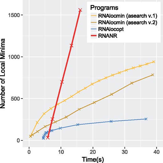
Comparison of local minima production speed for the SV11 RNA switch L07337_1 (115 nt). Experiment reproduced from Kucharik et al. (2014)
2 Approach
We introduce the concept of non-redundant sampling to study RNA kinetics, using locally optimal secondary structures as representative structures. Working with a reduced conformation space allows to mitigate the limitations of existing (redundant) sampling approaches. The problem of constructing all locally optimal secondary structures was addressed in Saffarian et al. (2012). Here, we describe an alternative generation algorithm which is efficient, and allows the specification of comprehensive structural restrictions (Section 2.2). We then define the first non-redundant sampling algorithm for locally optimal RNA structures (Section 2.3), allowing for the exploration of RNA folding landscape. The two algorithms are implemented within the standalone software RNANR.
2.1 Definitions
An RNA sequence w is a nucleotide sequence of length n over the alphabet . The symbol at position i is denoted by . A secondary structureS is set of pairs of positions in w, called base pairs, that are pairwise juxtaposed or nested. Specifically, if two base pairs (i, j) and are such that , then either or . This definition implies that a secondary structure is non-crossing, or pseudoknot-free, and each position is involved in at most one base pair. As a consequence, it can be encoded by a dot-parenthesis expression, where each base pair is a pair of matching brackets and unpaired positions are reprented by a dot. We also require that each pair (i, j) in S is valid, i.e. is in . Given a base pair (x, y), we denote the helix of length p stemming from (x, y): this is the set of base pairs .
2.1.1 Structural restrictions
The set of secondary structures on a given sequence can be further restricted by enforcing additional constraints, giving rise to more realistic structures. Those restrictions include: a) the minimum helix lengthα. In particular, isolated base pairs are forbidden for any value ; b) the maximum number of consecutive unpaired bases in the structure β; c) the maximum number of branches within a multiloop , which defines the maximum allowed number of outermost base pairs within another base pair; d) the minimum length of a hairpin loopθ. These parameters are illustrated on Figure 2. The special case α = 1, and θ = 1 corresponds to the whole set of secondary structures.
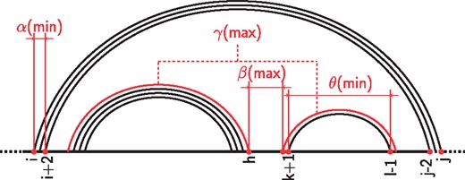
Graphical representation of the structural restrictions supported by RNANR. α is the lower bound on the size of helices. θ is the minimum length of a hairpin. γ limits the maximum number of branches within multiloops. Finally, β is the maximum number of nucleotides in unpaired regions
Subsequently, we will use as a shorthand for this search space, i.e. the restriction of secondary structures that respect those parameters. Within this search space, we define the neighborhood of a secondary structure S as the subset of secondary structures on w that can be obtained by adding or removing a single base pair in S.
2.1.2 Energy models
For a given secondary structure S on w, we associate a free energyES, computed with respect to a specific energy model. In this work, we consider two energy models. The first model is a simple base-pairing model where the energy is the number of base pairs. We call it the Nussinov model in the spirit of (Nussinov and Jacobson, 1980), even if structural restrictions introduced in the preceding paragraph significantly reduce the set of secondary structures. The second model is the 2004 version of the Turner thermodynamic model (Turner et al., 1988; Turner and Mathews, 2010). For a given free energy model, we say that a secondary structure is locally optimal if, and only if, it has minimal free energy within its neighborhood. We respectively denote by and the sets of locally optimal secondary structures (LOSSes) with respect to the Nussinov and Turner energy models, and will respectively refer to them as Nussinov LOSSes and Turner LOSSes in the following.
2.1.3 Thermodynamic concepts
2.2 Building LOSSes in the restrained Nussinov model
In Saffarian et al. (2012), it is shown that locally optimal secondary structures without structural restrictions can be built from substructures that are maximal by juxtaposition, called here flat structures in short. We elaborate on this idea in order to account for the expressive set of structural restrictions introduced in Section 2.1.
2.2.1 Flat structures
For any interval in w, a flat structure f is a sequence of juxtaposed (non-nested) helices which is maximal, meaning that it cannot be completed by a valid base pair between the positions left accessible by the helices. In other words, let be positions in w, such that and such that is a valid helix for each k, . This sequence of helices is a flat structure f on if, and only if: for each secondary structure S on containing f, if (x, y) is in S and not in f, then (x, y) is nested in (xk, yk) for some . We further assume that and to meet the requirements on β, δ and θ. We denote by such a flat structure, assuming that . We denote by the complete set of flat structures associated with the region in w, as illustrated by Figure 3. When an interval is not associated with any flat structure, we have (ε is the empty flat structure) whenever , and (empty set) otherwise. can be computed using a dynamic programming scheme adapted from Section 3.1.2, Theorem 2 in Saffarian et al. (2012).
![Examples of flat structures. For the structural parameters α = 2, δ = 3, θ = 1 and γ = 3, the set F1,18 of flat structures associated with the interval [1,18] consists of the five flat structures f1⋯f5. Note that h2(1,7)⊕h2(8,14) does not meet the condition on γ, as positions 15 and 18 are left unpaired, and thus is not a valid flat structure](https://oup.silverchair-cdn.com/oup/backfile/Content_public/Journal/bioinformatics/33/14/10.1093_bioinformatics_btx269/7/m_bioinformatics_33_14_i283_f3.jpeg?Expires=1749937942&Signature=c8YYx~b~H9s8wemtVSNiQgAsyvGFz-z9uhQvudZDOM1rH8f6VbroHcRr10Xw9NVyPIx0tIS3sXqI~clr6-mSf9TscMZN4aF-mCTUXLXGK9YsPN7Ly5N~xVQsI9ksWAuf6DDDICVh3Rws~PY6x0BijQ91WA93xCHD49VqGIsz~O6IH6Lda8bpF05KYKjswz9b6WpoqjdqJ~VotFMKdpPdO7DGxPxGhAN6h3Wy6xZf1LfLFMHX0RST8zsDBFUoN4tmRhZUVRQarVtcg3AjnvyupvP8CCugqXUJU7Nwbqh4XM58mE1qB9FoZhYpYJZuzy4yLzUHx2Pb5gG8yPfXvNP~Yg__&Key-Pair-Id=APKAIE5G5CRDK6RD3PGA)
Examples of flat structures. For the structural parameters α = 2, δ = 3, θ = 1 and γ = 3, the set of flat structures associated with the interval consists of the five flat structures . Note that does not meet the condition on γ, as positions 15 and 18 are left unpaired, and thus is not a valid flat structure
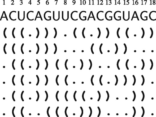
All locally optimal secondary structures of generated by the grammar Gw for the sequence, and using structural restrictions, described in Figure 3
2.2.2 A grammar for
Now comes the crucial observation that any locally optimal secondary structure of can be built up from a set of flat structures, completed with helix extensions as illustrated byFigure 4. Given a helix of length p, an extension is the addition of the valid base pair to form . The dot-parenthesis notations for the set of all structures of associated with an RNA w can be modeled as a context-free language generated by the grammar , where
is the set of non-terminal symbols. represents all locally optimal substructures within the interval , and represents the choice between a helix extension with the base pair (i, j) or starting a new substructure on the same interval;
is the set of terminal symbols;
- R is the set of production rules:(P1)(P2)(P3)
is the start symbol.
This grammar has non-terminal symbols and productions. The proof of its completeness with respect to can be adapted from the proof of Theorem 1 in Saffarian et al. (2012).
The condition in P3 ensures that Gw is unambiguous, and can be used as a conceptual template to derive other algorithms, e.g. to compute the partition function (Waldispühl and Clote, 2007) or base-pairing probabilities. Here, we use it on two related applications: exhaustive enumeration of structures and non-redundant statistical sampling of structures. While the former can be obtained in a straightforward fashion, being the language of the grammar, the latter is more involved and is the object of the next section.
2.3 Non-redundant sampling algorithm
The large redundancy of stochastic sampling methods has been identified by previous studies as one of the major shortcomings of existing methods. Ah hoc heuristics, such as the ξ-scheduling technique inspired by simulated annealing, have been introduced to circumvent such limitations, sometimes at the cost of a control over the sampled distribution (Kucharik et al., 2014). Here, we propose another approach based on an explicit avoidance of redundancy within the sampling, adapting principles introduced by Lorenz and Ponty (2013).
: Choose with probability and backtrack over the triplet , otherwise append the base-pair (i, j) to the output, and backtrack over ;
- : Choose a flat structure with probability
Note that the sets are explicitly computed, and so are the probabilities pf of choosing any flat structure f during the backtrack. It is thus possible to order the flat structures in by decreasing probability, leading to a substantial speed-up during the backtrack.
2.3.1 Non-redundant sampling
The stochastic backtrack becomes much more involved in the presence of a predefined set of forbidden structures, e.g. singled out to avoid redundancy, as the probabilities of the backtrack on disjoint intervals can no longer be considered independent.
As a minimal illustration, consider two intervals I1 and I2 where local sets of substructures and can be respectively chosen, leading to the generation of 6 different structures. Clearly, in the absence of forbidden sets, one simply needs to choose uniformly within each set to draw each structure with probability 1/6, i.e. in the uniform distribution. However, if a given combination of structures has to be avoided, say , then the choice over I1 now influences the valid combinations, and thus the probabilities, of choosing a structure over I2. Namely, choosing for I1 only allows access to 2 viable alternatives for I2, while choosing S1 for I1 enables 3 alternatives over I2. In order to be uniform, a stochastic backtrack must therefore choose S1 with probability 3/5, and with probability 2/5. Once chosen, the remaining choice is uniform over if S1 is chosen (prob.), or over (prob.) if is chosen.
More generally, in order to pick local alternatives in a way that is consistent with a predetermined distribution, one needs to access (or compute) the overall mass of forbidden structures that can be generated before and after the choice. The idea of Lorenz and Ponty (2013) consists in maintaining a dedicated data structure μ, which enables efficient access to the overall count/weight of accessible forbidden structures from the current state f the backtracking stack T.
The modified non-redundant backtrack is similar in structure to the classic one, but uses different derivation probabilities, starting from a stack . Let denote the overall number/weight of structures accessible from a given state. At each iteration, it extracts a triplet (i, j, m) from T:
- If , choose with probabilitywhere and backtrack over , or otherwise backtrack over , after adding (i, j) to the output;
- If , choose a flat structure with probabilitywhere , and backtrack over the stack after adding the chosen f to the output.
In practice, both the data structure μ and the N(T) can be updated on-the-fly during the backtrack, so that the non-redundancy retains the same asymptotic complexity as the redundant one.
2.3.2 Turner energy model and expressive structural restrictions
The various contributions of the loops in the Turner energy model can easily be identified in the grammar. Namely, stacking pairs are generated by rule (P1), while rule (P2) generates terminal loops (hairpins) when , internal loops and bulges when , or multiple loops when . Finally, the exterior loop corresponds to .
This enables the incorporation of Boltzmann weights, based on the Turner energy model as weights in each of the DP equations. The incorporation of such weights during the stochastic (non-redundant) backtrack leads to an algorithm for Boltzmann sampling, whose details and (sketch of) proof of correctness are provided in Supp. Mat. 1.
3 Materials and Methods
All experiments were run on a laptop with Intel Core i7 5600 CPU equipped with a quad core at 2.6 GHz with 16 GB of RAM under Ubuntu 16.04 LTS.
RNANR was implemented in C, and is freely available. It interfaces the RNALib, using the C ++ API provided in the Vienna package (Lorenz et al., 2011), to access the individual contributions of the 2004 version of the Turner energy model. The tests were done on a version compiled with gcc using GNU99 standard.
Gradient walks were performed used the move_gradient function of the ViennaRNA package (Lorenz et al., 2011), which performs a gradient descent in the Turner energy landscape and return one of the closest local minima.
3.1 Datasets
Three datasets were considered in our validation effort. The uniform dataset consists in random, uniformly distributed, RNA sequences of length from 10 to 140 nt increasing by 10 nt, with 50 samples per length.
In order to assess the characteristics of real RNAs, we also gathered the RNAStrand dataset, which consists of the 154 RNA sequences of length between 120 and 170 nt downloaded from RNAStrand database (Andronescu et al., 2008), filtering out undefined symbols.
Finally, since currently available kinetics data is too scarce to allow for a quantitative comparison of tools, we created a dataset of 250 bistable sequences of length 100 nt. A bistable RNA sequence presents two stable conformations differing by a sufficient number of base pairs. We generated random uniform sequences of length 100 nt, and retained only those whose most stable LOSS (MFE) had free-energy lower than -30 kcal.mol–1 according to RNAEval (Lorenz et al., 2011). Remaining sequences were then subjected to non-redundant sampling of 1000 LOSSes using RNANR. We finally kept the sequences which, within the sampled set, featured an alternative metastable LOSS, differing by 20 base-pairs from the MFE structure, and having free-energy kcal.mol–1 higher than the MFE.
3.2 Program parameters
Unless noted otherwise, the settings of the different programs used in our comparisons are those described in this section.
For RNANR, the default mode is that of non-redundant sampling, with 20 samples. The structural restrictions include a minimum helix length α = 3, a minimal base pair distance θ = 3, a maximal unpaired region length δ = 7, and a maximal number of helices in multiloop β = 4.
For RNALocopt the number of returned samples is the same and the temperature was set to 310.15K.
For RNASLOpt, the suboptimality percentage was set to 100%, meaning that all LOSSes with energy ranging between the MFE and 0 are returned. Since we are interested in LOSSes independently of their stability, we set the barrier_cutoff to an arbitrarily large value of 30 kcal.mol–1 to speed up the computations by avoiding the computation of the energy barriers. Likewise, the number of top stable LOSSes can be chosen arbitrarily, here its value is set to 3.
RNALocmin was run using the second version of the built-in adaptative search script, referred to as asearch and coded in Python (Kucharik et al., 2014). The parameters used are those by default, i.e. 10 000, 10 and 0.1 respectively for the number of samples per iteration, number of iterations and convergence parameter.
3.3 Theoretical speed-up of non-redundant sampling
We propose a closed-form formula to quantify the speed-up factor induced by non-redundant sampling, i.e. the average number of occurrence of each unique samples. Let us consider a fixed sequence of i unique structures, and let Ri be the number of structures, generated by a redundant Boltzmann sampling algorithm, before returning a novel i + 1-th structure.
3.4 Time benchmarking RNANR against its competitors
We reproduced, and report in Figure 1, the benchmark of Kucharik et al. (2014) which compares the rates at which different sampling methods produce unique local minima. It focuses on the SV11 L07337_1 RNA switch, a challenging 115 nt RNA whose landscape is particularly deep and steep. For RNANR, the total number of generated samples was . RNALocmin was run using both first and second versions of asearch for maximum of 30 iterations. For both tools, the sampled structures are not necessary Turner LOSSes, so a gradient walk is performed, and duplicates were removed. The time spent by the gradient walk is added to the generation time in the benchmark. Finally, the total number of samples generated by RNALocopt was set to . Other parameters were the same as those specified above.
3.5 Comparison of folding landscape analysis efficiency
To compare the quality of sampled sets of structures, we considered an artificial bistable dataset described in Section 3.1, and produced representative sets of structures using the four programs mentioned in Section 3.2. We analyzed sampled sets using a standard kinetic analysis pipeline based on an estimation of energy barriers for each pair of structures, followed by a numerical integration using treekin.
For each sequence in the bistable dataset, each program was used to generate = 50, 75 and 100 samples (output truncated if necessary). Gradient walks were performed to each sample set, and duplicated Turner LOSSes were removed. As a control, we also included the results of RNAsubopt -e, adjusting to return at least LOSSes. Next, we estimated the energy barriers using the single path heuristics implemented by the findpath tool (Flamm et al., 2001). Due to the high computational cost of this operation, we restricted it to pairs of states having base-pair distance at most . For each sequence, the value of was set in such a way that landscapes sampled by all tools were connected (with the possible exception of RNAsubopt).
Finally, we considered a scenario where the starting concentration of the metastable structure (or its closest neighbor in the sampled set) is set to 1. We used treekin to determine the evolution of the concentration of all LOSSes in the sampled set. Finally, we report the switching time, i.e. the time at which the MFE structure eventually achieves higher concentration becomes more frequent than the metastable structure.
4 Discussion
4.1 Validating Nussinov LOSSes as key landmarks of kinetic landscapes
4.1.1 Nussinov LOSSes are less numerous than Turner LOSSes
We compared the numbers of LOSSes returned by RNANR, RNALocopt and RNASLOpt. For each sequence in the uniform dataset, these sequences were subjected to runs of each software. For RNANR, we performed three runs, each with different value of γ (no limit, 4 and 3 respectively). For RNALocopt and RNASLOpt we performed one run for each with parameters as specified in 3.2. The values of each run were then aggregated by the sequence length. The results are shown on Figure 5.
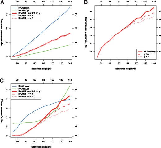
Comparison of RNANR with RNALocopt and RNASLOpt. (A) Number of structures returned by each program and in case of RNANR, for different upper limits of γ. (B) Number of flat structures returned by RNANR for different values of γ. (C) Benchmark for different programs, for the same cases as (A)
Figure 5A shows the evolution of number of LOSSes for different programs in function of sequence length. We observe that RNASLOpt returns the smallest number of results. This is consistent with the primary objective of Li and Zhang (2011) to reduce the number of structures as a way to reduce the complexity. Besides aggressive structural constraints, RNASLOpt returns only LOSSes that have negative free energy, which is not the case for both RNANR and RNALocopt. On the other hand, RNANR presents a lower number of solutions than RNALocopt. This stems both from the reduction of search space by RNANR due to the structural restrictions, and to our focus on Turner LOSSes, while RNALocopt arguably considers a larger neighborhood (Lorenz and Clote, 2011). Our search space reduction, while not as aggressive as that of RNASLOpt, leads to a substantial reduction of the complexity, both theoretically and practically, as shown in Figure 5.
Of interesting note is the comparison between the numbers of flat structures returned by RNANR for different values of γ (Fig. 5B). While the number of flat structures noticeably decreases for lower values of γ, the number of LOSSes does not seem to be particularly affected (Fig. 5A). This could be explained by the fact the excluded flat structures participate in few of the complete LOSSes, as substantiated by the fact that, for shorter sequences, the formation of multiloops with high number of branches is improbable. This interpretation is consistent with an analysis of RNAStrand structures (Fig. 6), which shows that very few (0.1%) RNAs of length under 140 nt features multiloops of degree greater than 4 branches. For shorter sequences, it thus seems reasonable to limit γ, which results in lowered time complexity. Naturally, as shown by Figure 6, this ceases to be the case for longer sequences. While for sequences shorter 300 nt the number of ignored structures for γ = 4 is still low (1.92%), for sequences shorter than 400 nt the number of multiloops with at least 5 branches accounts for 15.82% of all structures. Overall, we found that setting γ to 5 constitutes a reasonable tradeoff, reducing the computation time while keeping the number of undetected LOSSes reasonable.
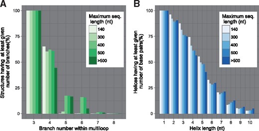
Rationale for our restricted search space. Effect of structural limitations on structure counts obtained from RNAStrand database (Andronescu et al., 2008). (A) Proportion of structures having maximal multi loop branches below a given threshold. A branch number within multi loop is the number of stems sorting from a multiloop and is equal to γ + 1. (B) Proportion of helices having at least given length
4.1.2 Nussinov LOSSes are very close to turner LOSSes
We used gradient walks to determine how distant are Nussinov LOSSes, output by RNANR, to their counterpart in the Turner energy model. For each sequence in the RNAStrand dataset, a non-redundant sampling of 1000 distinct structures was performed by RNANR. These structures were then subject to a gradient descent, resulting in a Turner LOSS. We tracked the modifications, both in term of energy and base pairs, induced by the walk. Our results are summarized in Table 1.
Discrepancy between Nussinov and Turner LOSSes
| Samples% | Base pair dist. | ||
|---|---|---|---|
| Avg (SD) | Avg (SD) | Avg (SD) | |
| Within search space | 59.57% (21.00) | 0.071 (0.309) | 0.129 (0.289) |
| Outside search space | 40.42% (21.00) | 1.248 (0.925) | 1.550 (0.619) |
| Global average | 100.00% (—) | 0.547 (0.817) | 0.703 (0.757) |
For our RNAStrand dataset, 1000 Nussinov LOSSes were generated. For each structure, one of the closest Turner LOSS was determined using a gradient descent. On average, a Nussinov LOSS is distant by ≤ kcal.mol–1, and by 0.7 base pairs, from its closest Turner LOSS.
Overall, 52.49% of the Nussinov LOSSes were already local minima with respect to the Turner energy model. Moreover, our analysis shows that, from a Nussinov LOSS, it is sufficient to add or remove an average of 0.703 base pairs, contributing an average 0.547 kcal.mol–1, to reach a Turner LOSS. A further analysis reveals differing behaviors of whether or not the Turner LOSS, obtained as the outcome of the gradient descent, belongs to the restricted search space.
Finally, it is worth stressing that the structures obtained after the gradient walk are overwhelmingly unique (99.1%), suggesting a homogenous coverage of the Turner LOSSes by the Nussinov LOSSes. We thus conclude that the structures generated by RNANR can reliably used as representatives for Turner LOSSes within the folding landscape.
4.2 Efficiency of sampling methods for LOSSes
A first time benchmark, whose results are given on Figure 5C was performed on our uniform dataset. We observe that, without limiting γ, RNANR is fastest for sequences of length under 80 nt. Around this length, it is briefly matched by RNASLOpt, whose execution time increases spectacularly around 110 nt. RNALocopt is faster than RNASLOpt or RNANR (no limitation on γ) for longer sequences (more than 120 nt) due to the polynomial nature of the underlying algorithm. However, for values of γ set to 3 or 4, the execution time of RNANR becomes polynomial, and RNANR becomes considerably faster in practice than its competitors. Of course, one needs to exercise caution before setting restrictions that could lead to the omission of important conformations, and it would probably not be wise to set γ = 3 for RNAs beyond 80 nt. However, setting γ = 4 makes RNANR faster than any other tested software, while only missing a negligible proportion of existing conformations (cf Fig. 6, for multiloop branch number equal to 6) for sequences beyond 300 nt.
A second basic time benchmark, described in Section 3.4 and in Figure 1, measures the rate of production of distinct Turner LOSSes generated using different software. We observe that RNANR returns more unique LOSSes in a given time, even when including the time for precomputations and gradient descents, than both versions of RNALocmin and RNALocopt (note that RNASLOpt does not perform sampling). This is mainly due to the redundancy within the returned samples, as indicated by the diminishing production speeds for both methods. The second version of asearch uses an alternative strategy for ξ-scheduling which increases its number of samples linearly between iterations, and seems to eventually perform better than its initial version. However it starts slower, proving that the redundancy is still an issue.
4.3 Non-redundant sampling allows a deeper exploration of kinetic landscapes
The main new contribution of RNANR is its non-redundant sampling algorithm, which allows to obtain a set of locally optimal secondary structures, each of whom appears at most once. This method of sampling has its advantages which will be discussed in this and next subsection. The more obvious one, discussed here, is the fact it allows to obtain higher number of different samples faster. Instead of sampling same structures with free energy close to the minimal free-energy over and over, it consecutively picks up the structures with higher energies which were not sampled previously.
To demonstrate this point, we first computed the value of speed-up T(k)∕k as defined in Section 3.3 on two sequences: a 123 nt 5S ribosomal RNA of Thermoplasma acidophilum, and a 154 nt telomerase RNA of Tetrahymena silvana. A non-redundant sampling was performed, until a coverage of 0.99% was achieved, and the evolution of the speed-up was calculated. The results are shown on Figure 7A and B. The purple dots mark the points with for , 1% and 0.1% for the final coverage.
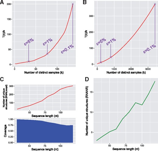
Comparison of classical and non-redundant sampling. (A) Theoretical speed-up T(k)∕k using non-redundant sampling when compared to redundant sampling for a 5S ribosomal RNA of Thermoplasma acidophilum (123 nt). (B) Same test for a telomerase RNA of Tetrahymena silvana (154 nt). Purple points indicate the coverage of , for and 0.1% respectively. (C) Number of unique LOSSes and coverage c from 1000 samples generated by RNALocopt on our uniform artificial dataset. The number of unique LOSSes, generated using RNANR in order to achieve a coverage c, is plotted in (D)
The value of T(k)∕k increases with k, which is expected since the probability of generating a novel structure decreases with each iteration. The speed-up thus becomes more important for higher values of c (or lower values of ), where the probability of a new unique structure almost vanishes. This means that the structures with higher free energies are considerably easier to generate by non-redundant sampling than by their redundant counterpart, since their initial probability increases along with the sampling. Moreover, different sequences exhibit different evolutions for c, as shown on Figure 7A and B, depending on the concentration of the Boltzmann distribution around a few conformations. This means that higher values of c will be more difficult to attain for some sequences than for others, and for these cases the usage of non-redundant sampling might prove more advantageous.
Our second test consisted in creating the samples using redundant generation, and comparing these results with the non-redundant sampler of RNANR. For this purpose, we used RNALocopt to generate 1000 LOSSes for each sequence of our uniform dataset. For each set of structures, the number of unique samples and the coverage c were computed. RNANR was then used to generate a set of structures achieving the same coverage c. The averaged number of structures for each length was reported, leading to the values shown in Figure 7C and D.
While the number of unique structures returned by RNALocopt increases with the sequence length, the coverage value c diminishes. This is caused by the increasing number of local minima for longer sequences, which results in lower Boltzmann probabilities for individual structures. This means that, to attain a given coverage c, a sharply increasing number of LOSSes must be generated for longer sequences, leading to a higher number of repeats. Figure 7D shows that the number of samples necessary to achieve identical c by RNANR as the one achieved by RNALocopt is considerably lower. This partially stems from the fact that while RNALocopt encompasses the entirety of Turner LOSSes, RNANR explores a much more drastically reduced search space, and thus requires less samples to achieve a given coverage. On the other hand, this also means that a target coverage is achieved faster while generating most of interesting structures with the correct parameter settings, meaning that RNANR can considerably speed up and simplify the analysis of the folding landscape.
4.4 Non-redundant sampling of Turner LOSS enables a faster, more accurate analysis of RNA kinetics
The main interest of non-redundant sampling is, besides its inherent speed-up, its capacity to dig deeper within the space of suboptimal structures when approximating the folding landscape of a given RNA. In this final validation, we tested whether this increased diversity translates into sampled sets of higher quality, leading to more accurate kinetics analysis.
More specifically, we evaluated the capacity of a simple, real-life, analysis pipeline to estimate the switching time of bistable artificial RNAs from samples of small size, generated using RNANR, RNALocmin, RNASLOpt, RNALocopt and RNAsubopt. Details are described in Section 3.5, and the results are summarized by Figure 8, and illustrated by Figure 9.
First, we observe that RNANR detects structures that are similar to both the MFE and metastable LOSSes more consistently than its competitors. This is not overly surprising, since these two structures were initially identified from an independent execution of RNANR (albeit from a much larger sampled set, see Section 3.1). This however means that RNANR generates sets of structures that, while not strictly overlapping, represent the main dominant conformations even for small sampled sets, and may be used for reproducible further analysis. RNALocmin and RNALocopt both suffered from redundancy, and generally failed to identify the two dominant conformation for about of the bistable RNAs. RNASLOpt exhibit the same tend, probably due to an aggressive filtering of LOSSes.
Then we compared the switching time, defined in Section 3.5, as predicted by our pipeline from the different sampled sets. We reasoned that, since both undersampled landscapes and single-path heuristics lead to an overestimation of energy barriers, a good sampled set, by populating important energy basins, would be associated to a fast perceived kinetics, i.e. a fast switching time. On the other hand, a set of scattered, or highly similar, structures would practically disconnect the landscape, leading to slow predicted kinetics. Faster predicted switching times therefore indicate better approximate folding landscapes.
Our results, summarized in Figure 8, show that using RNANR leads to the shortest switching time ∼70% of the time, irrespectively of the number of samples. RNASLOpt is a clear second, and dominates other tools with respect to the switching time in about 20% of the sequences. While high computational demands, on both the design and analysis tasks, disallowed us to repeat this on larger bistable sequences, we expect this trend to carry for larger sequences and sets.
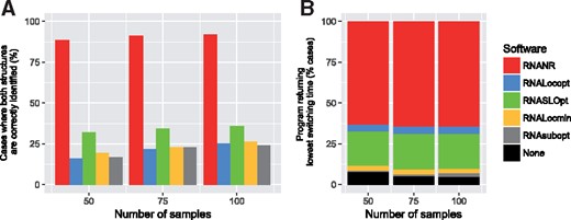
Efficiency of analysis performed by existing sampling software on bistable structures. (A) Proportion of artificial bistable sequences for which structures close to the reference states are generated. (B) Distribution of best-performing software, as assessed by the lowest predicted switch time, for different values of
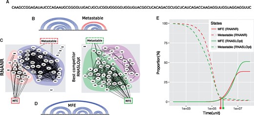
Illustration of bistable RNA analysis. Starting from an artificial 100 nt bistable RNA (A), metastable (B) and MFE (D) states are identified, along with key landmarks of the kinetic landscapes, using the non-redundant sampling of RNANR (C, left) and RNASLOpt (C, right). Due to the stochastic nature of the landscape reconstruction methods, the metastable structure identified by RNANR has 3 extra base pairs (B, colored in red). Numerical integration of the master equation using Treekin (D) predicts a shorter switching time for RNANR kinetics landscape than its competitors, suggesting a better coverage of important kinetic intermediate structures
Acknowledgements
The authors wish to thank Ronny Lorenz and Gregor Entzian for their invaluable help in interfacing the versatile Vienna RNAlib, and Ivo Hofacker for his feedback and suggestions at an earlier stage of this work.
Funding
All authors acknowledge support from the RNALands project, jointly funded by the French Agence Nationale de la Recherche (ANR-14-CE34-0011) and the Austrian Fonds zur Förderung der wissenschaftlichen Forschung (FWF-I-1804-N28).
Conflict of Interest: none declared.
References

