Modeling and comparing the organization of circular genomes

Abstract

1 INTRODUCTION

Most of the prokaryotic genomes (1158 out of 1194, NCBI, August 2010) are circular with a single chromosome (called circular genomes henceforth). Orthologous genes (abbreviated as orthologs) are genes directly evolved from an ancestor gene (Tatusov et al., 1997), and can be traced through different species in evolution. The fraction of shared orthologs between two circular genomes was found to be better conserved than the order of genes (Huynen and Bork, 1998), in which the fraction of shared orthologs between genomes was employed to measure genome evolution of nine prokaryotes. Here, our emphasis is on the structure of circular genomes, which, for example, plays an important role in synthetic biology. A review paper in synthetic genomics (Carrera et al., 2009) indicates that genome organization may influence gene expression, which is vital for organisms. Further, predicting or modeling the rules of genome organization via comparative genomics may provide valuable information for genome construction.

We reason that genome structure can be studied via distributions of shared orthologs between genomes, e.g. the most or least favored region in which shared orthologs between each pair of bacterial genomes are located. While the marginal distributions of shared orthologs are often found to be asymmetric and bimodal, to date there is no joint distribution with closed-formed marginals to model such data. This motivated us to develop a family of joint distribution and its related statistical inferences.

Recent studies show that gene order is extensively conserved between closely related species, but rapidly become less conserved among more distantly related species. This trend is likely to be universal in prokaryotes (Tamames, 2001; Wolf et al., 2001). However, the fraction of shared orthologs between two circular genomes is more conserved than the order of genes (see Fig. 6 of Huynen and Bork, 1998). In addition to the fraction of shared orthologs between bacterial genomes, we further incorporate the distributions of shared orthologs of paired circular genomes to infer similarity of their genome organization. By converting the locations of shared orthologs in any paired circular genomes into angles, these pairs of angles can be viewed as bivariate circular vectors.

Most of the marginal distributions of shared orthologs in circular genomes are asymmetric and/or multimodal, which can be modeled by the generalized von Mises distribution (GVM) (Maksimov, 1967; Yfantis and Borgman, 1982). Therefore, we propose a family of bivariate circular distributions with each marginal assuming a GVM distribution, and call this family the bivariate generalized von-Mises (BGVM). The inference procedures, estimation of the parameters in BGVM and testing for independence of structures of paired circular genomes, are developed. A novel correlation measure, which is based on the fraction of shared orthologs and a circular grade correlation derived here, is introduced to measure organization similarity between circular genomes. Furthermore, this similarity is visually depicted by the rose diagrams of shared orthologs.

The marginal distributions of BGVM are quite flexible since GVM can model either symmetric or asymmetric, unimodal or multimodal circular data, depending on the values of its four parameters. The probability density function (pdf) of GVM is in closed form and thus is convenient for inferences; see Yfantis and Borgman (1982) for details.

In the following, we briefly review literature on modeling bivariate circular data, e.g. shared orthologs of paired prokaryotic genomes. Thompson (1975) mentioned the wrapped bivariate normal distribution. Mardia (1975) proposed a generalized von Mises–Fisher model for paired angles (θ₁, θ₂). Wehrly and Johnson (1980) generated families of bivariate circular distributions with jpdf:

(1)

where 0 ≤ θ₁, θ₂ < 2π, g, f₁ and f₂ are densities on the circle, and F₁ and F₂ are the distribution functions of f₁ and f₂, respectively. The pdf in Equation (1) has f₁ and f₂ as its specified marginals. Shieh and Johnson (2005) studied a family of bivariate distributions, belonging to these families in Equation (1), with von Mises marginals and its inferences. Rivest (1988) investigated inferences for a bivariate generalization of the Fisher–von Mises distribution. Unfortunately, the marginals of these distributions are symmetric and unimodal, hence they cannot be employed to model distributions of shared orthologs in paired circular genomes. Bivariate circular distributions with asymmetric and/or multimodal but closed-formed marginals have not been well explored, thus we study them here.

2 METHODS

Here, we investigate inference procedures under BGVM which has the probability density function:

(2)

where 0 ≤ θ₁, θ₂ < 2 π, κ₁₂ ≥ 0, 0 ≤ μ₁₂ < 2π and I₀(·) denotes the modified Bessel function of the first kind and order zero. These GVM marginals assume the forms

where C_j⁻¹ = 2π {I₀(κ_j)I₀(λ_j) + 2 ∑_n=1^∞I_n(λ_j)I_2n(κ_j) · cos[2n(μ_j − ν_j)]}. These μ_j and ν_j (κ_j and λ_j) are location (dispersion) parameters, and we denote this GVM distribution as GVM (μ_j, ν_j, κ_j, λ_j) henceforth. The joint density BGVM involves the cumulative distributions F_j(θ₀) = ∫₀^θ₀f_j(θ)dθ, but with todays computing power this is not a serious drawback. We note that this class of bivariate circular distributions can include other marginals, e.g. t-distribution (Shimizu and Iida, 2002), von Mises distribution (Shieh and Johnson, 2005) and Jones and Pewsey's distribution (Jones and Pewsey, 2005).

2.1 Roles of some parameters in the BGVM model

The parameters κ and λ in a GVM (μ, ν, κ, λ) marginal control not only the concentration at θ = μ and θ = ν but also the graphic shape of the density. If κ = 0, the GVM is antipodally symmetric and has two modes, depending on λ, at θ = ν and θ = ν ± π. If λ = 0, the GVM reduces to the von Mises distribution, which is symmetric and unimodal, with mean direction μ and concentration κ; the larger κ is the more concentrated when the distribution is at μ. If μ₁₂ = 0 , the BGVM is a unimodal distribution, and as κ₁₂ increases the association between Θ₁ and Θ₂ increases, which indicates that the association between the given pair of circular genomes increases. From the copula representation in Section 2 of Shieh et al. (2006), we have that Φ₁ = 2π F₁(Θ₁) given θ₂ is VM (μ₁₂ + 2πF₂ (θ₂), κ₁₂). When μ₁₂ = 0, Φ₁ centers on 2πF₂(θ₂), and the dependence of Θ₁ on Θ₂ is controlled by the magnitude of κ₁₂.

A BGVM generator written in R is available at http//:www.stat.sinica.edu.tw/∼gshieh/bgvm.htm.

2.2 Estimation and testing hypothesis under a BGVM distribution

2.2.1 MLEs of the parameters

Assuming that shared orthologs between a pair of circular genomes follow a BGVM distribution, given their converted angles we can immediately obtain the fitted BGVM distribution by applying the MLE algorithm in MLE_LR-test.R of the Supplementary Material. The MLE algorithm was modified from the Newton–Raphson method (Tanner, 1996), to prevent the estimates for the model in Equation (2) being trapped in local maxima, which was caused by the sinusoidal functions in the joint density. Next, we derive the limiting distribution of MLEs for the parameters in BGVM. The likelihood ratio test for independence of the organization between genomes is addressed at the end of this section.

To see how the MLE algorithm performs, we show its estimation results using data generated from BGVM with the parameters (μ₁, ν₁, κ₁, λ₁, μ₂, ⁠, and the sample size 100. We first estimated parameters of the marginals and obtained and ⁠. Next, we used these estimates as initial values and applied the MLE algorithm to estimate parameters of the joint density. The estimates obtained are ⁠, = (1.33, 1.65, 0.92, 0.95, 1.62, 1.55, 1.02, 0.90, 0.92, 2.32), which are quite close to the true values.

After the MLEs been computed, estimates of their variances and covariances can be obtained from derivatives of the likelihood or by numerical integration of the squares and products of the partial derivatives given in Section 3 of Shieh et al. (2006). Let η = (μ₁, ν₁, κ₁, λ₁, μ₂, ν₂, κ₂, λ₂, μ₁₂, κ₁₂)^T be the vector of 10 unknown parameters. The parameter space is then

for i = 1, 2. Let l_n(η) denote the log-likelihood function, and U_n(η) and −I_n(η) the first and the second derivatives of l_n(η), respectively.

When the vector of parameters η belongs to the interior of the parameter set, the regularity conditions (see Section 3 of Shieh et al., 2006 for details) hold, and the consistency of the MLEs follows, which implies that the vector of MLEs multiplied by converges to their true parameters. Asymptotic multivariate normality of the MLEs then follows from Lemma 1 and Theorem 2 of Self and Liang (1987), which indicates that this centered vector converges to a multivariate normal distribution as stated below.

Theorem 1.

Let η belong to the interior of the parameter set. The vector of MLEs has multivariate normal limiting distribution, and

where I is the Fisher information matrix with entries

The 10 partial derivatives are straightforward and are omitted.

Remark

Numerical integration can be used to obtain each of the entries I_ik's. However, this could be difficult and it is better to use the estimated, or empirical, information with terms

where each partial derivative is evaluated at the MLEs. Different asymptotics apply if we include κ₁₂ = 0 in the parameter space. If κ_i and λ_i,i = 1, 2 are still bounded away from 0, then according to the results in Self and Liang (1987), Theorem 2 and Case 2 of page 606, has limiting distribution Z₁I[Z₁ > 0 ] , where Z₁ has a normal distribution with variance determined from I⁻¹. The cases where κ₁ = 0, λ₁ = 0, κ₂ = 0 and/or λ₂ = 0 are treated similarly.

2.2.2 Testing for independence of the organization between circular genomes

To test the hypothesis that the organization of paired prokaryotic genomes are independent or not, e.g. whether the structure organization of Thermotoga and that of Sulfolobus are independent, we consider likelihood ratio tests (LR tests), which include two cases. In both cases, under the BGVM joint distribution this test is equivalent to testing

The likelihood ratio statistic is −2lnλ_n, where

Δ₀ = {μ₁, μ₂, ν₁, ν₂, κ₁, κ₂, λ₁, λ₂}, and Δ₁ = {μ₁, ν₁, μ₂, ν₂, μ₁₂, κ₁, κ₂, λ₁, λ₂, κ₁₂}.

There are really two cases, and the second case is the most complicated.

Case 1. When all parameters are unknown and none of κ₁, λ₁, κ₂, λ₂ are zero. The limiting distribution of −2ln λ_n is

where χ_r² denotes the chi-square distribution with r degrees of freedom, by Case 5 of Self and Liang (1987).

Case 2. When all parameters are unknown and only one among κ₁, λ₁, κ₂ and λ₂ is zero. In practice, this case occurs when MLEs of the four parameters are close to zero. The limiting distribution of −2ln λ_n is

where ⁠, I_ij's are the (i, j) entries of the information matrix I(η) and c₂ = c₃ = 1/4 − c₁. Furthermore,

f(x, y, α) = [(x² + y²)^1/2 − x sinα]/cosα and Φ(·) is the standard normal cumulative distribution function. For details, see Case 8 of Self and Liang (1987).

Codes in R to obtain MLEs and the LR test are available at http://www.stat.sinica.edu.tw/∼gshieh/bgvm.htm.

2.3 A novel circular correlation measure r_pg

Huynen and Bork (1998) used the fraction of shared orthologs between genomes to study genome evolution. The ratio of shared orthologs between a pair of genomes to the maximum possible number of shared orthologs, which is estimated by the size of the smaller genome in each pair of genomes, is a reasonable index for association of organization between circular genomes. This ratio (denoted by r_p) can be written as

To characterize association between a pair of circular genomes more finely, the similarity of their distributions of shared orthologs should be taken into account. This association can be measured by a circular grade correlation (r_g) derived in the next subsection. Weighting both r_p and r_g equally gives rise to a novel circular correlation measure

Note that there is a parameter, namely protein sequence similarity, involved when choosing one-to-one orthologs between genomes. The rule of thumb is to choose a protein sequence similarity value such that r_p and r_g are of the same scale, e.g. 0.7 was suggested for the threshold of protein sequence similarity in a pilot study, in which the BGVM procedures were applied to the nine prokaryotic genomes in Application 1.

2.3.1 A circular grade correlation measure r_g

When the joint pdf of two r.v.'s on the real line, say X₁ and X₂, involves the marginal cumulative distributions F_i(X_i), i = 1, 2, the grade correlation (ρ_H) (Hoeffding, 1948) was shown to be suitable for correlation of X₁ and X₂. This correlation measure is defined as

Recall that (Θ_1k, Θ_2k), k = 1, …, n, denote the mapped angles of n pairs of shared orthologs between prokaryotic Genomes 1 and 2. When the joint pdf of these pairs of angles involves the marginal cumulative distributions F_i(θ_i), i = 1, 2, a suitable correlation may be modified from the grade correlation ρ_H. Similar to previous works on deriving association measures for bivariate circular data (Shieh et al., 1994; Shieh and Johnson, 2005), a new circular grade correlation coefficient for bivariate circular data, that allows for different choices of the origins in each genome, is

where F_i(Θ_i) is uniformly distributed on [0, 1], for i = 1, 2, and mod(Θ₂ + δ) denotes Θ₂ + δ (mod 2π). Via some computation in Appendix1.pdf of the Supplementary Material, we obtained that the circular grade correlation

The MLE for the circular grade correlation ρ_g assumes the following form.

where A = { 2π · i/n : i = 0, 1,…, n − 1}, is the MLE of the F₂ marginal distribution and and are MLEs for κ₁₂ and μ₁₂.

2.3.2 The large sample (limiting) distribution of r_g

For each pair of genomes, the number of shared orthologs can range from a few hundred to more than two thousand. With such large sample sizes, the limiting distribution of the circular grade correlation estimate r_g in general follows a normal distribution. To provide confidence intervals for ρ_g to judge whether the similarity on distributions of shared orthologs of paired circular genomes is different from zero (independence) or not, we derive the limiting distribution of the centered r_g.

Because r_g is the MLE of ρ_g, the large sample distribution of r_g follows a normal distribution with its covariance matrix computed from angles of shared orthologs. That is,

where the covariance matrix D² can be computed by our code,

and are derived in Appendix2.pdf of the Supplementary Material, which provides a proof for the convergence of the centered r_g to a normal distribution.

The 1 − α confidence interval of ρ_g(θ₁, θ₂) is [r_g − Z_α/2D, r_g + Z_α/2D], where 0 < α < 1 and Z_α/2 is the critical value of the standard normal distribution N(0, 1) at the level of α/2.

2.3.3 A visualization tool: rose diagrams

To visually depict association between paired circular genomes, we applied rose diagrams (a kind of angular histogram; Fisher, 1993) to each pair of shared orthologs. The radius of each sector with a binwidth of 10^○ or other angles is proportional to the relative frequency of shared orthologs, whose corresponding angles belong to the sector, e.g. 60^○ ∼ 70^○ of the rose diagram of Sulfolobus in Figure 1, where the inner dotted (outer) circle denotes the frequency being 10 (20). In general, a small binwidth results in a bumpier rose diagram than that of a large one.

Fig. 1.

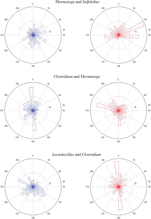
The rose diagrams of shared orthologs, identified by protein sequence similarity 0.7, of three pairs of prokaryotic genomes.

Open in new tabDownload slide

3 RESULTS

In this section, we apply the proposed procedures to shared orthologs between paired prokaryotic genomes to measure similarity of their genome organization. However, we note that our procedures can be applied to many features of genomic organization, e.g. shared TFBSs, shared repeated elements (Benson and Waterman, 1994) and shared non-coding genes (e.g. rRNA and small RNA), by inputting their corresponding angles instead of those of shared orthologs to our algorithm. For instance, both Escherichia coli and Bacillus subtilis have more verified TFBSs than other bacteria, and we can analyze their shared TFBSs using procedures developed here.

3.1 Data preprocessing

To let the shared orthologs between paired circular genomes reflect their similarity, we filtered out predicted horizontal transferred genes. The filtering was performed using data from the Horizontal Gene Transfer Database (Garcia-Vallve et al., 2003), which were accessed at http://genomes.urv.es/HGT-DB/. After the filtering, only species-specific genes were left in each circular genome, and we mapped their physical positions into angles ranged in [0, 2π). As an ortholog in each circular genome has a clustered orthologous group (COG) ID (Tatusov et al., 1997), the genes having the same COG ID in any paired circular genomes were identified as orthologs.

Paralogous genes (abbreviated as paralogs) are genes related by duplication within a genome. Due to gene duplication, there may be orthologous sets of paralogs within one genome, and several paralogs may share the same COG ID. That is, there are one-to-many, many-to-one and many-to-many corresponding shared orthologs besides the one-to-one corresponding ones. Using the following minimum angle distance, we can identify one-to-one shared orthologs. Let D(A, B) denote the distance between orthologs A and B, and D(A, B) = min{|angle of A − angle of B|, 2π − |angle of A − angle of B|}. For an orthologous set (multiple paralogs with the same COG ID), we use the shortest distance ortholog pairs (A, B), where D_min(A, B) = min_i,jD(A_i, B_j) and 1 ≤ i ≤ m, 1 ≤ j ≤ n, provided that m and n are orthologs in genomes A and B corresponding to one COG ID.

Let θ_ij and θ_kj for 1 ≤ j ≤ n, denote the corresponding angle of the first base of the shared ortholog j in genomes i and k, which were used for statistical inferences. Note that within any given pair of genomes, the locations of distinct ortholog pairs are assumed to be independent and identically distributed (i.i.d.) samples. Because marginals of shared ortholog genomes were often found to be asymmetric and bimodal, we fitted a BGVM model to each pair of shared orthologs for the prokaryotic genomes studied.

In the following, we apply the proposed BGVM procedures and rose diagrams to two sets of prokaryotic genomes, consisting of eight pairs of prokaryotic genomes separated from domain down to species, and 13 mycoplasma bacteria which are mammalian pathogens belonging to the same genus.

3.2 Application 1: eight pairs of prokaryotic genomes separated from domain to genus

In this application, we compare the structure organizations for each of the following pairs of bacterial genomes, which are (Thermotoga, Sulfolobus), (Clostridium, Thermotoga), (Lactobacillus, Clostridium), (Staphylococcus, Lactobacillus), (Oceanobacillus, Staphylococcus), (Bacillus, Oceanobacillus), (Bacillus anthracis, Bacillus subtitlis) and (Bacillus anthracis Ames, Bacillus anthracis Sterne). These pairs of genomes belong to different domains, the same domain, phylum class, order, family, genus and the same species, respectively. Among them, we first tested whether the genome structures of each pair are independent or not. After using the threshold of 0.7 for protein similarity to identify shared orthologs between each pair of genomes, we plotted their rose diagrams, which showed that several of the marginals are bimodal. Due to a space limit, only the rose diagrams (using a binwidth of 10^○) of the first three pairs are presented in Figure 1; see Supplementary Figure S1 in Application1.pdf for all rose diagrams. Some marginal distributions of these pairs of bacterial genomes were asymmetric, based on the result of the test for symmetry in Pewsey (2002). For instance, some marginals of (Thermotoga, Sulfolobus), (Clostridium, Thermotoga) and (Lactobacillus, Clostridium) are asymmetric at the 95% significance level; see Table 1 for details.

For asymmetric and bimodal marginals of shared orthologs, it was reasonable to fit GVM distributions. Goodness-of-fit was checked by QQ-plots, similar to those in Shieh et al. (2006), which indicated that the fits were adequate for the marginals. For the fitted GVMs and QQ-plots, please see the file at http://www.stat.sinica.edu.tw/∼gshieh/bgvm.htm. The asymmetry and bimodality of the marginals suggested fitting a BGVM to shared orthologs for each pair of prokaryotic genomes. The MLE estimates of parameters in BGVM of (Thermotoga, Sulfolobus), (Clostridium, Thermotoga) and (Lactobacillus, Clostridium) are given in Table 2.

Table 2.

Open in new tab

The shared orthologs of three pairs of circular genomes, identified by protein sequence similarity 0.7, fitted by BGVM models

Genome (i, j) .	.	.	.	.	.	.	.	.	.	.
(6, 7)	0.32	0.27	3.14	1.79	0.31	0.49	5.78	3.05	0.68	0.62
(7, 8)	0.28	0.40	5.39	3.13	0.13	0.31	4.87	2.25	0.28	6.21
(8, 9)	0.20	0.11	2.19	0.30	0.58	0.61	0.24	1.33	0.18	5.49

Genome (i, j) .	.	.	.	.	.	.	.	.	.	.
(6, 7)	0.32	0.27	3.14	1.79	0.31	0.49	5.78	3.05	0.68	0.62
(7, 8)	0.28	0.40	5.39	3.13	0.13	0.31	4.87	2.25	0.28	6.21
(8, 9)	0.20	0.11	2.19	0.30	0.58	0.61	0.24	1.33	0.18	5.49

Due to space limit, we use genome numbers 1–9 to represent the following nine prokaryotic genomes, respectively: Bacillus anthracis Ames, Bacillus anthracis Sterne, Bacillus subtilis, Oceanobacillus, Staphylococcus, Lactobacillus, Clostridium, Thermotoga and Sulfolobus.

Table 2.

Open in new tab

The shared orthologs of three pairs of circular genomes, identified by protein sequence similarity 0.7, fitted by BGVM models

Genome (i, j) .	.	.	.	.	.	.	.	.	.	.
(6, 7)	0.32	0.27	3.14	1.79	0.31	0.49	5.78	3.05	0.68	0.62
(7, 8)	0.28	0.40	5.39	3.13	0.13	0.31	4.87	2.25	0.28	6.21
(8, 9)	0.20	0.11	2.19	0.30	0.58	0.61	0.24	1.33	0.18	5.49

Genome (i, j) .	.	.	.	.	.	.	.	.	.	.
(6, 7)	0.32	0.27	3.14	1.79	0.31	0.49	5.78	3.05	0.68	0.62
(7, 8)	0.28	0.40	5.39	3.13	0.13	0.31	4.87	2.25	0.28	6.21
(8, 9)	0.20	0.11	2.19	0.30	0.58	0.61	0.24	1.33	0.18	5.49

Due to space limit, we use genome numbers 1–9 to represent the following nine prokaryotic genomes, respectively: Bacillus anthracis Ames, Bacillus anthracis Sterne, Bacillus subtilis, Oceanobacillus, Staphylococcus, Lactobacillus, Clostridium, Thermotoga and Sulfolobus.

Employing the LR-test based on the distributions of shared orthologs, we test whether genome organization of each pair of these prokaryotes are independent. (Not) rejecting this hypothesis indicates that their genome organizations are (not) correlated. For each pair of prokaryotic genomes, a LR-test of shared orthologs was computed, and the result showed that except (Thermotoga, Sulfolobus), the hypothesis was rejected for the other seven pairs at a 95% level using Case 2; see Application1.pdf of the Supplementary Material for details. This result indicates that for these seven pairs, their genome organizations are correlated based on the similarity of the distributions of their shared orthologs. This association can also be seen easily from their rose diagrams, in particular those of Bacillus anthracis Ames and Bacillus anthracis Sterne.

Next, we estimated the association of genome organizations of each of the eight pairs of prokaryotes. Note that the origins of most prokaryotic genomes are unknown (and having no rules to predict) or predicted, which demonstrates the importance of r_pg's being invariant to the origins of both circular genomes. The values of r_p, r_g and r_pg of these pairs (in Table 3) are incidentally consistent with their phylogeny relationships. The rose diagrams show that the genome structures of Bacillus anthracis Ames and Bacillus anthracis Sterne are almost identical, while those of Thermotoga and Sulfolobus are not at all alike.

3.3 Application 2: 13 mycoplasma bacteria

Above we showed that the BGVM distribution and its inference procedures can be applied to distinguish genome organization of eight pairs of bacteria in Application 1, in which genomes of six pairs were relatively distant (from different genus or beyond). Here, we apply the proposed procedures to a set of 13 mycoplasma bacteria, which are relatively close in phylogeny, to see if r_pg can distinguish their genome organization. These bacteria are mammalian pathogens with small genomes, which belong to the same genus. Specifically, their phylogeny tree based on 16S ribosomal sequence, constructed by the software MEGA4, is in Application2.pdf of the Supplementary Material. Among these bacterial genomes, three origins are unknown and nine are predicted, which demonstrates the need of a correlation measure invariant to the origin of a circular genome such as r_pg.

The pairwise rose diagrams (with a binwidth of 10^○) of these 13 bacterial genomes showed that several of the marginals were bimodal and asymmetric; see http://www.stat.sinica.edu.tw/∼gshieh/bgvm.htm for details. Hence, we fitted a BGVM distribution to the shared orthologs for each pair of bacterial genomes. Next, the correlation measure r_pg was applied to these genomes to result in the values in Table 4.

Interestingly, these associations are consistent with those measured based on similarity of their 16S rRNAs. Among these 13 bacterial genomes, the top few correlated pairs in terms of r_pg are (M.genitalium G37, M.pneumoniae M129), (M.hyopneumoniae J, M.hyopneumoniae 7448), (M.hyopneumoniae 232, M.hyopneumoniae 7448) and (M.hyopneumoniae 232, M.hyopneumoniae J), whose values are equal to 0.77, 0.71, 0.69 and 0.67, respectively. The latter three pairs are hyopneumoniae, which cause chronic disease in pigs and attach to the same organ (lung cilia). From the rose diagrams of these hyopneumoniae in Figure 2, we can see that their genome structures are quite similar in terms of shared orthologs. The most favored regions of their shared orthologs are 80^○ − 90^○, (20^○ − 30^○ and 330^○ − 340^○) and (20^○ − 30^○ and 330^○ − 340^○), respectively, in which 23, (16 and 17) and (14 and 16) genes are in common, respectively. Among these genes, the largest common functional group is translation, and their gene orders are also conserved. For details, please see Supplementary Tables S1 and S2 in Application2.pdf. In particular, the rose diagrams of (M.hyopneumoniae J, M.hyopneumoniae 7448) clearly depict their similarity in genome organization, and the most and least favored regions of shared orthologs are 80^○ − 90^○ and 150^○ − 160^○, respectively. The genes located in the most favored region, encode ribosomal subunit proteins 30S and 50S, which are essential genes and are known to cluster together to form an operon structure in many bacterial genomes (Bratlie et al., 2010).

Fig. 2.

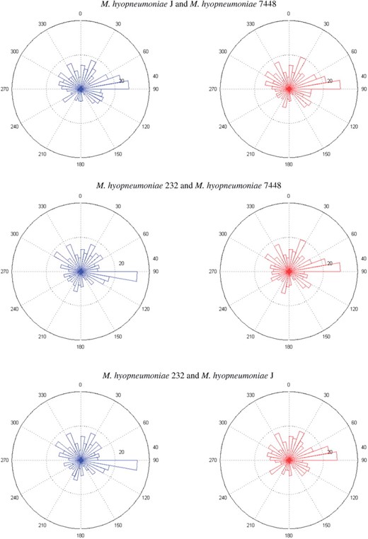
The rose diagrams of shared orthologs, identified via protein sequence similarity 0.7, of three pairs of hyopneumoniae bacteria.

Open in new tabDownload slide

Moreover, the aforementioned relationships depicted by rose diagrams are consistent with those of the other analysis on genome organization (Application2.pdf of the Supplementary Material). Thus, our procedures may provide useful information on comparing the organization of circular genomes and genome construction in synthetic biology.

4 DISCUSSION

The proposed BGVM distribution, with flexible and closed-formed marginal distributions, was shown to model paired angular data well, in which each marginal of the pair can be asymmetric or/and multimodal, e.g. shared orthologs between paired bacterial genomes. Statistical inferences employing the MLEs for parameters of the BGVM distribution and the LR-test for independence of the organization between circular genomes are established. A novel circular correlation measure (r_pg), invariant to the choices of origins of circular genomes which are mainly unknown or predicted, was derived and a visualization tool provided. We applied these procedures to two sets of prokaryotic genomes, consisting a set of relatively distant prokaryotes and a set of closely related bacteria. The novel correlation measure r_pg was shown to summarize associations between prokaryotic genomes well. While the rose diagrams further depict their associations via distributions of the shared orthologs. Our results are consistent with those of other analysis. Thus, the BGVM procedures may provide useful information on the organization of circular genomes.

We note that the BGVM procedures can be applied to identify shared TFBSs, shared coding or non-coding genes and shared repeated elements between circular genomes. Thus, they may be applied to identifying conserved chromosome backbones, detecting conserved gene clusters such as operons, among others, which can be used for genome construction in synthetic biology.

ACKNOWLEDGEMENTS

We are indebted to Jia-Hong Wu and Su-Wei Hsu for computational assistance; Shih-Chung Chuang for statistical assistance. We thank Chuang-Hsiung Chang for discussions, and the AE and two reviewers for constructive comments that improved this article.

Funding: Shurong Zheng was supported by a postdoctoral fellowship from Academia Sinica thematic grant (23-33); the research was supported in part by National Science Council, Republic of China (96-2118-M-001-010-MY2) and National Research Program-Genome Medicine grant (NSC99-3112-B-001-015) for G.S.S.

Conflict of Interest: none declared.

REFERENCES

Author notes