


In their paper in Bioinformatics, Mitchell et al. (2004) constructed a model of single nucleotide polymorphism (SNP) genotyping errors in different studies, and based on this model concluded that our study (Carlson et al., 2003) missed 99% of heterozygous genotypes when the minor allele was present only in the heterozygous state. We show here that this oversimplified model strikingly fails to fit many descriptors of our data, such as nucleotide diversity and allele frequency distribution, and that the results of Mitchell et al. are based on an incorrect value of one of the two statistics that they used to describe our data.
Mitchell et al. stated that the best fit to our data was obtained with a model in which 99% of all heterozygous genotypes are wrongly called as homozygous for all SNPs with the minor allele observed only in the heterozygous state. This model makes several predictions about our data, which could have been tested by Mitchell et al. because the data are publicly available on our website (http://pga.gs.washington.edu). All of these predictions are in striking disagreement with the data. The model predicts an allele frequency spectrum for the detected SNPs that is radically different from the allele frequency spectrum observed in our data (Fig. 1). In a simulated sample of 94 chromosomes under a standard neutral model (Hudson, 2002) (100 regions of 500 000 bp simulated assuming constant population size, uniform recombination at 1 cM per Mb, and 4Nμ = 8.0 × 10⁻⁴), 59% of all SNPs were observed only in the heterozygous state; so, the model predicts that we would have missed 57% of all SNPs and 79% of SNPs with minor allele frequencies <20%. The missed rare SNPs would decrease the nucleotide diversity (Watterson's θ) by more than half in the simulated data from 8.1 × 10⁻⁴ to 3.4 × 10⁻⁴ (Table 1). In fact, the observed nucleotide diversity (θ) in our data was 9.6 × 10⁻⁴, consistent with other large-scale surveys of sequence diversity (Halushka et al., 1999; Cargill et al., 1999). Missed rare sites also reduced nucleotide diversity (π) in the simulated data from 8.1 × 10⁻⁴ to 6.1 × 10⁻⁴. The nucleotide diversity (π) of our data was 7.5 × 10⁻⁴, again consistent with other large-scale surveys of sequence diversity. The model predicts a striking excess of high-frequency sites, reflected by a significantly positive value of Tajima's D (D = 2.7) in the simulated data. In fact, the observed value of Tajima's D in our data was −0.79, reflecting a non-significant trend toward an excess of low-frequency sites. The model predicts that only 5.5% (<1% excluding singletons) of the detected SNPs would have the minor allele present only in the heterozygous state. In fact, 68% (51% excluding singletons) of the detected SNPs had the minor allele present only in the heterozygous state. Finally, the model predicts that among these SNPs, we would rarely make a heterozygous genotype call more than once and never more than twice. In fact, we observe a distribution of the number of heterozygous genotype calls ranging from 1 to 25 (Fig. 2). All of these observations are consistent with a low rate of false-negative genotype calls, and are completely inconsistent with the model of Mitchell et al.
The model of Mitchell et al. includes two parameters, ε2 and ε4, which represent the false-positive rate and the false-negative rate (when the minor allele is observed only in the heterozygous state), respectively. We ran our simulations with the parameter ε2 set to zero because this is the value reported by Mitchell et al. (Table 4 of their paper), but including nonzero values of ε2 in the simulations does little to improve the fit. The ε2 parameter does not fix the fact that models with high values of ε4 produce a highly distorted frequency spectrum inconsistent with our data. It merely adds a large number of false-positive singleton SNPs to the predicted dataset, which does nothing to fix the dearth of SNPs with low and intermediate minor allele frequencies generated by the model. Table 1 shows values of a number of summary statistics for our dataset, a model with ε2 and ε4 set to zero (which fits all aspects of the data quite well), and models with a range of values for ε2 (with ε4 = 0.99). While non-zero values of ε2 allow individual statistics to be fit better, no value provides a good overall fit. The best-fit model for Tajima's D is around ε2 = 2e − 5, but this model produces a deficit of SNPs with low and intermediate minor allele frequencies and a large excess of singletons (Fig. 3). Additionally, this model underestimates nucleotide diversity and fails miserably to match the observed fraction of SNPs with multiple observations of the minor allele only in the heterozygous state (Table 1). The two values that most closely match our observed nucleotide diversity (ε2 = 5e − 5 and ε2 = 1e − 4) also produce a deficit of SNPs with low and intermediate minor allele frequencies (Fig. 3) and heterozygous SNPs (Table 1), and a huge excess of singletons. Additionally, these three models incorporating ε2 predict that 52–84% of the SNPs in our sample are false positives, far above the rates we have estimated (0.1%) from confirmatory genotyping on alternate technical platforms. In this respect, it is interesting to note that Mitchell et al. hypothesized that their prediction of a high false-negative rate for our dataset was a consequence of ‘a higher standard for accepting heterozygous calls’, i.e. a low false-positive rate.
How did Mitchell et al. obtain a model that so strikingly fails to fit our data? One obvious explanation is that they fitted two summary statistics of the different studies, but used an incorrect value of one of the two statistics for our dataset. This statistic is the fraction of confirmed SNPs that are common. For other studies, Mitchell et al. defined ‘common’ as minor allele frequency >10% in the overall combined study sample. Using this definition, 79% of our confirmed SNPs are ‘common’, consistent with the other studies (73–79%). For our study, they defined ‘common’ as minor allele frequency >10% in either of the two populations we studied, which is a more inclusive definition and leads to a higher fraction of ‘common’ SNPs. Under this incorrect definition, 85–89% of our confirmed SNPs are ‘common’. The use of an inappropriately high fraction of ‘common’ SNPs among the detected SNPs would lead one to erroneously conclude that many SNPs with low minor allele frequency were missed. Thus, in addition to the inherently flawed predictions of the model for the observed allele frequency spectrum, the modeling exercise was also invalid because one of the two model parameters used to describe our dataset was fundamentally inaccurate.
It is worth noting that Mitchell et al. also used an incorrect value of the other summary statistic, the SNP confirmation rate, for the study of Reich et al., (2003). They quoted rates of 93 and 98% for the BAC- and TSC-derived SNPs, respectively. The correct rates are 74 and 94%, respectively, and the higher values are obtained only when the locus with the lowest confirmation rate is removed from the dataset. Again, the use of incorrect model parameters for the Reich dataset leads to an absurd prediction from the model of Mitchell et al. In order to explain the discrepancy between their estimated 16–17% false-positive rate for putative dbSNPs and the 2–7% non-confirmation rate of Reich et al. (which suggests that they ‘confirmed’ many false-positive dbSNPs), Mitchell et al. estimate a 0.7% probability of wrongly calling the major allele as the minor allele in the study by Reich et al. While this probability seems small, it in fact means that in analyzing 150 chromosomes, Reich et al. would have called monomorphic sites polymorphic ∼65% of the time. Such a high-false-positive SNP rate would imply that in 173 kb of sequence, Reich et al. would have called approximately 113 000 sites polymorphic, rather than the 923 variant sites they reported.
In conclusion, theoretical models are only valuable insofar as they generate testable predictions that provide meaningful insights. The model of Mitchell et al. is fundamentally flawed because it is based on incorrect parameters for two out of three datasets, with the consequence that it generates predictions that are easily rejected by a cursory inspection of the data. While variation does exist among the reported dbSNP confirmation rates in these three reports, this model fails to provide meaningful insight into the origin of this discrepancy.
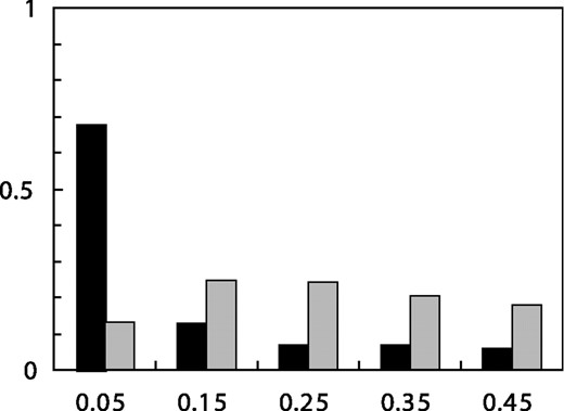
Frequency distribution predicted by Mitchell et al. in gray compared with the actual values of our data shown in black. We obtained quantitative predictions of the model by running 100 coalescent simulations of SNP discovery in 94 chromosomes, using a constant population size and nucleotide diversity of 8.0 × 10⁻⁴. Following the model of Mitchell et al., the true genotypes generated by the coalescent simulations were altered by replacing heterozygous calls with homozygous calls with a probability of 0.99 if the minor allele was observed only in the heterozygous state; allele frequency and other statistics in the text were tabulated only for the sites that remained polymorphic after this procedure.
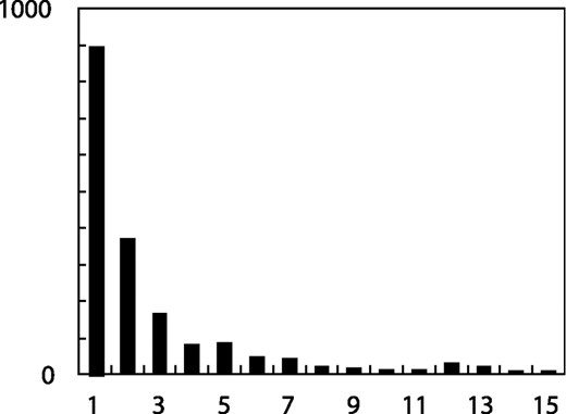
Number of SNPs without the minor allele observed in the homozygous state plotted against the number of minor allele observations.
Comparison between Carlson data and Mitchell model
| Data ε2 | ε4 | Nucleotide diversity (π) | Nucleotide diversity (θ) | Fraction false positives | Fraction singletons | Tajima's D | Fraction heterozygous SNPsa |
|---|---|---|---|---|---|---|---|
| 0 | 0 | 0.00081 | 0.00081 | 0 | 0.20 | 0.01 | 0.498 |
| 0 | 0.99 | 0.00061 | 0.00034 | 0 | 0.05 | 2.70 | 0.002 |
| 1e − 7 | 0.99 | 0.00061 | 0.00035 | 0.01 | 0.06 | 2.67 | 0.002 |
| 5e − 7 | 0.99 | 0.00062 | 0.00035 | 0.03 | 0.08 | 2.55 | 0.002 |
| 1e − 6 | 0.99 | 0.00062 | 0.00036 | 0.05 | 0.10 | 2.41 | 0.002 |
| 5e − 6 | 0.99 | 0.00062 | 0.00044 | 0.21 | 0.25 | 1.49 | 0.002 |
| 1e − 5 | 0.99 | 0.00063 | 0.00053 | 0.35 | 0.38 | 0.70 | 0.002 |
| 2e − 5 | 0.99 | 0.00065 | 0.00071 | 0.52 | 0.54 | −0.27 | 0.003 |
| 3e − 5 | 0.99 | 0.00067 | 0.00089 | 0.61 | 0.63 | −0.84 | 0.004 |
| 4e − 5 | 0.99 | 0.00069 | 0.00108 | 0.68 | 0.70 | −1.22 | 0.006 |
| 5e − 5 | 0.99 | 0.00071 | 0.00126 | 0.73 | 0.74 | −1.48 | 0.008 |
| 1e − 4 | 0.99 | 0.00081 | 0.00217 | 0.84 | 0.85 | −2.15 | 0.028 |
| 5e − 4 | 0.99 | 0.00161 | 0.00929 | 0.96 | 0.94 | −2.84 | 0.382 |
| 1e − 3 | 0.99 | 0.00261 | 0.01783 | 0.98 | 0.94 | −2.94 | 0.702 |
| (Carlson et al.) | 0.00075 | 0.00096 | 0.001b | 0.33 | −0.79 | 0.511 |
aFraction of SNPs with the minor allele observed only in the heterozygous state, after removing the singletons.
bEstimated from confirmation by independent techniques.
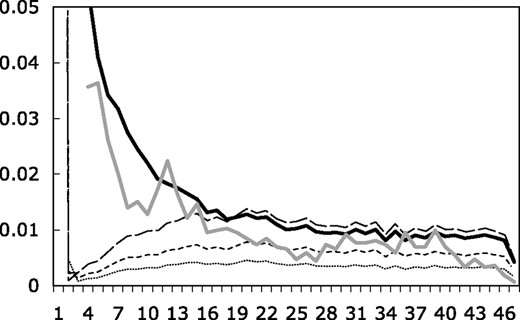
Fraction of all SNPs with a given number of observations of the minor allele for models with ε2 = 0.0001 (dashed line), ε2 = 0.00005 (dotted line) and ε2 = 0.00002 (dashed-dotted line), as well as error-free simulated data (solid black line) and the data of Carlson et al. (solid gray line). We have cut off the y-axis for the singleton bin (minor allele observed only once). The singletons comprise 85 (ε2 = 0.0001), 74 (ε2 = 0.00005) and 54% (ε2 = 0.00002) of all SNPs in these simulations. The singletons comprise 20% of SNPs in the error-free simulated dataset and 33% in our data.
REFERENCES
Mitchell, A.A., Zwick, M.E., Chakravarti, A., Cutler, D.J.
Carlson, C.S., Eberle, M.A., Rieder, M.J., Smith, J.D., Kruglyak, L., Nickerson, D.A.
Hudson, R.R.
Halushka, M.K., Fan, J.B., Bentley, K., Hsie, L., Shen, N., Weder, A., Cooper, R., Lipshutz, R., Chakravarti, A.
Cargill, M., Altshuler, D., Ireland, J., Sklar, P., Ardlie, K., Patil, N., Lane, C.R., Lim, E.P., Kalayanaraman, N., Nemesh, J., et al.

