


Abstract
Missing values (MVs) can adversely impact data analysis and machine-learning model development. We propose a novel mixed-model method for missing value imputation (MVI). This method, ProJect (short for Protein inJection), is a powerful and meaningful improvement over existing MVI methods such as Bayesian principal component analysis (PCA), probabilistic PCA, local least squares and quantile regression imputation of left-censored data. We rigorously tested ProJect on various high-throughput data types, including genomics and mass spectrometry (MS)-based proteomics. Specifically, we utilized renal cancer (RC) data acquired using DIA-SWATH, ovarian cancer (OC) data acquired using DIA-MS, bladder (BladderBatch) and glioblastoma (GBM) microarray gene expression dataset. Our results demonstrate that ProJect consistently performs better than other referenced MVI methods. It achieves the lowest normalized root mean square error (on average, scoring 45.92% less error in RC_C, 27.37% in RC_full, 29.22% in OC, 23.65% in BladderBatch and 20.20% in GBM relative to the closest competing method) and the Procrustes sum of squared error (Procrustes SS) (exhibits 79.71% less error in RC_C, 38.36% in RC full, 18.13% in OC, 74.74% in BladderBatch and 30.79% in GBM compared to the next best method). ProJect also leads with the highest correlation coefficient among all types of MV combinations (0.64% higher in RC_C, 0.24% in RC full, 0.55% in OC, 0.39% in BladderBatch and 0.27% in GBM versus the second-best performing method). ProJect’s key strength is its ability to handle different types of MVs commonly found in real-world data. Unlike most MVI methods that are designed to handle only one type of MV, ProJect employs a decision-making algorithm that first determines if an MV is missing at random or missing not at random. It then employs targeted imputation strategies for each MV type, resulting in more accurate and reliable imputation outcomes. An R implementation of ProJect is available at https://github.com/miaomiao6606/ProJect.
INTRODUCTION
Missing values (MVs) refer to information points being present in some samples but not others. They are also referred to as ‘missing data’ or ‘data holes’ [1]. MV is thought to make up approximately 50% of the MS/MS-based proteomic data, while the percentage of proteins with at least one MV can reach 90% [2]. The presence of data holes hinders the complete and accurate extraction of quantitative and functional information, particularly for tasks such as differential analysis, machine learning or drug prediction. Consequently, addressing MV appropriately poses a significant challenge for proteomic studies [3].
MVs pose a critical issue in high-throughput data analysis, as they can result in unreliable outcomes and poorly trained predictive models. Real-world applications, such as biomarker discovery or personalized medicine, rely on accurate data interpretation, making MV handling essential. Mishandling MVs can seriously compromise data analysis, resulting in wrong selection of data features (false positives) or lead to mis-trained machine-learning models. MVs are dealt with using a range of techniques known collectively as missing value imputation (MVI). To date, an extensive library of MVIs has been developed [1]. MVs abound across various high-throughput technologies and are seen as an important problem. Thus, there are benchmarking studies identifying best MVI methods across various platforms such as genomics [4], proteomics [5], metabolomics [6] and even clinical trials [7].
There are different kinds of MVs, each with its unique characteristics (and causes) and requiring a different MVI approach. MVs are categorized into three types: missing at random (MAR), missing not at random (MNAR) and missing completely at random (MCAR). In general, MCAR refers to missing data that are unpredictable and are neither data nor platform dependent (e.g. randomly incomplete derivatization or ionization [6]). MNAR MVs, on the other hand, are associated with actual values of the missing data and can depend on data-specific or platform-specific factors. For example, MNARs that come about due to detection limits are usually also associated with low-abundance issues (e.g. in a data-dependent acquisition process, only the most abundant ions are selected for analysis during the MS2 stage [8]). MAR do not depend on the missing value itself, but instead on other sub-variables from the same data, such as sample- or batch-related information (e.g. different class of data may be dependent on specific experimental treatments, with the likelihood of MV being influenced by these factors). In proteomics, actual values of MAR and MCAR MVs often exhibit correlation with other values in high-dimensional datasets. Therefore, from an MVI perspective, MAR/MCAR are often regarded as the same.
Existing MVI methods can be categorized into three main types: single-value approaches, local-similarity approaches and global-structure approaches.
Single-value approaches, such as MEAN imputation, handle MVs in a naïve way by replacing the MVs with a constant, random value, or in this case, the mean.
Local-similarity approaches, on the other hand, impute MVs based on the similar intensity neighbors in the same dataset. K-Nearest neighbors (KNN) and local least squares (LLS) are popular techniques for this form of MVI. KNN is a simple supervised machine-learning method that selects the most similar neighbors based on Euclidean distance and subsequently replaces the MV with the weighted average of the neighbors. Similarly, LLS selects the nearest neighbors by calculating the Pearson correlation coefficient, then performs a linear regression to determine the imputation value. Both KNN and LLS were developed to handle MAR/MCAR MVs. Thus, to accommodate MNAR MVs, methods have also been developed to impute for left-censored data. For example, KNN-Truncation (KNN-TN) is a modification to KNN, which assumes that the distribution of the complete data follows a truncated normal distribution. Like LLS, the Quantile Regression Imputation of Left-Censored data (QRILC) is another regression-based method. However, it uses quantile regression to estimate parameters for a left truncated normal distribution before randomly drawing values from this distribution for MVI.
Finally, global-structure approaches apply dimensional reduction methods to decompose the dataset and then reconstruct the missing values. For example, probabilistic principal component analysis (PPCA) and Bayesian principal component analysis (BPCA) are two methods that make use of the eigenvalue decomposition of the matrix using PCA, combined with an expectation maximization (EM) approach, and incorporates either a probabilistic model or Bayesian model, respectively. These MVI methods reconstruct MVs based on the reduced features such that the major dimensions of the data are retained.
However, whether a single-value, local-similarity or global-structure approach is used, most MVIs from any of these categories face three significant challenges. First, most MVI methods are primarily designed for either MAR/MCAR or MNAR, with very few capable of handling mixed MVs (combinations of MAR, MCAR and MNAR). This limitation is problematic since real-world data are usually composed of mixtures of various MVs, rendering these MVI methods impractical or error prone. KNN-TN is one of few MVI methods capable of dealing with mixed MVs [9]. Although it deals with both MNAR and MAR, its reliance on nearest neighbors may cause inaccurate imputation in the presence of batch effects, strong class effects or high variations between samples.
Second, most MVI methods perform stably only when the sample size is large [10]. Although dimensionality reduction methods, such as PPCA and singular vector thresholding, perform well on genomic datasets with hundreds of samples [11, 12], they falter on proteomic datasets, where sample sizes tend to be smaller. A good MVI should have a robust algorithm such that it works well on any given data size. Furthermore, the ‘curse of dimensionality’ arises when feature size is much larger than sample size, as is often the case in proteomic datasets. Most proteomic datasets have large feature sizes (thousands) with relatively small samples (tens). This imbalance can lead to bias when algorithms cannot precisely filter out unrelated information. This consequence becomes more obvious when the missing rate (the proportion of MVs in the data against the entire data matrix) is low, and many irrelevant features are included in the model. Feature-based methods, such as decision trees and simple regression models, lack a regulated process to filter irrelevant features, exacerbating this problem.
Lastly, some MVI methods, particularly parameter-based algorithms, assume that the data follow a certain distribution, which leads to limited usage scenarios. For example, EM and certain PCA-based algorithms estimate parameters based on normality assumptions [11, 13], while KNN-TN and QRILC assume a truncated normal distribution [6, 14]. When base data assumptions do not hold, subsequent parameter estimation will fail to correctly estimate the MVs.
To address these challenges, we designed ProJect (short for Protein inJection), a novel mixed-model imputation method that can deal with mixed missingness, is not limited by sample size and does not require data to follow a specific distribution. ProJect provides accurate imputation results across various scenarios. It has been evaluated on two proteomics datasets and two genomics datasets using multiple evaluation criteria, with stable and satisfactory performance outcomes.
MATERIALS AND METHODS
We used four datasets, ovarian cancer (OC), renal cancer (RC), which is further separated to RC full dataset and RC_C dataset, BladderBatch and glioblastoma (GBM) dataset for benchmarking. All datasets have been condensed to a sub-dataset with no MVs. Simulated MVs are then inserted artificially from 10 to 40%, constituting various missing scenarios. For each missingness scenario, we evaluated five distinct combinations of MAR and MNAR, or MCAR and MNAR. We compare ProJect against seven other state-of-the-art methods: QRILC [14], KNN [15], PPCA [11], BPCA [16], LLS [17], KNN-TN [9] and MEAN. Detailed descriptions of the other MVI methods are provided in Supplementary Table 1 and Supplementary Description.
Datasets
Renal cancer acquired using DIA-SWATH
The renal cancer (RC) DIA-SWATH data of Guo et al. [18] contains a group of 24 runs of 12 kidney tissues obtained from 6 patients with clear cell renal cell carcinoma. For each patient, one tumorous and one non-tumorous tissue are collected. Each sample has two technical duplicates. The SWATH map is generated by TripleTOF 5600 MS operated in SWATH acquisition mode. All SWATH runs are processed by OpenSWATH, and the library search is performed against a kidney tissue SWATH assay library. The SWATH assay library contains 49 959 reference spectra. In total, under a precursor false discovery rate (FDR) of 0.1% cutoff, 2375 proteins were identified from the union of samples and had 36% MVs. There are two assigned data classes in the RC dataset; tumorous samples are designated as RC cancer (RC_C), while non-tumorous samples are designated as RC normal (RC_N). In our experiment, we use RC cancer and full RC data (the union of RC_C and RC_N data).
Ovarian cancer dataset acquired using DIA-MS
The ovarian cancer (OC) dataset is a reduced dataset derived from previous literature [19]. A set of 20 high-grade serous ovarian cancer patients diagnosed with Stage III/IV disease is used in this study. The chromatograms are extracted and assigned using OPENSWATH, with a FDR of identification <1% in at least one dataset file. The individual patient tumor proteomic dataset is downloaded from ProteomeXchange (ID PXD023040). The OC dataset is a subset of the patient tumor dataset, from which we only extracted tumor samples that contained at least one technical replicate. The OC dataset contains 9 samples, with 6077 proteins identified and around 7% missingness.
Bladder (BladderBatch) microarray gene expression dataset
The BladderBatch [20] package contains microarray gene expression data that can be used to examine the gene expression patterns in superficial transitional cell carcinoma (sTCC) with and without surrounding carcinoma in situ (CIS) [20]. The data contain gene expression data of 57 samples that have been normalized with Robust Multi-array Average (RMA) and pre-processed according to a previously defined protocol [21]. To test an MVI method’s ability to distinguish different classes and batches, our benchmark extracts the first 16 samples, with 8 normal samples and 8 cancer samples from three different batches. Of the cancer samples, four of them are sTCC samples with CIS and four of them are sTCC samples without CIS. For faster simulation, we only include randomly 2000 genes for analysis.
Glioblastoma microarray transcriptomic dataset
The glioblastoma (GBM) dataset, as detailed by Gerber et al. [22], provides comprehensive transcriptome data from seven long-term survivors (LTS) who lived beyond the expected 48 months after their GBM diagnosis. The LTS patients’ transcriptomes reveal a distribution across diverse GBM subtypes, including proneural (n = 2), neural (n = 2), classical (n = 2) and mesenchymal (n = 1). The Affymetrics U133 2.0 microarray was employed to perform a meticulous expression analysis of the tumors. The gene matrix can be found in GEO database [23] with accession number GSE54077. To ensure the efficiency of our experiment, we focused our analysis on a subset of 2000 genes, chosen at random. Given the dataset’s structure of three classes spread over seven samples, we limited our analysis to include only MCAR and MNAR simulations.
ProJect algorithm
ProJect comprises four steps: sample scaling, input matrix construction, mixed-model imputation and outlier optimization. A simple workflow is shown in Figure 1.
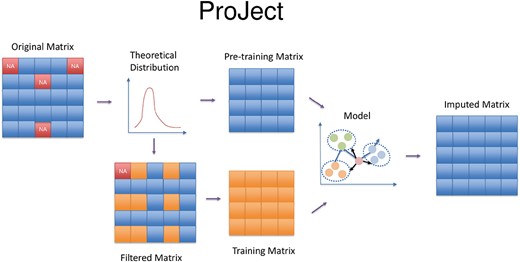
ProJect algorithm workflow. The theoretical distribution is generated to provide a basis for the imputation of missing values in a matrix. To facilitate this process, the original matrix is split into two components: a pre-training matrix, which is used to train the model parameters, and a filtered matrix, which serves as input to the model. The missing values are then replaced by the prediction of the model and formed the imputed matrix.
Previous methods often assume normality for data fitting [11, 13]. However, based on our observations and previous literature, the sample typically does not strictly follow a typical normal distribution. For example, KNN-TN uses truncated normal for metabolic samples [9], and Combat-seq assumes RNA data follow a negative binomial distribution [24]. Directly assuming normal distribution and calculating mean and standard deviation can lead to bias as it ignores the MVs’ distribution. Our observations suggest that using skew normal distribution provides a better fit for the data.
To address non-normality, we first generate a skewed normal distribution, which generalizes the normal distribution to allow for non-zero skewness. The scaling parameters are estimated using maximum penalized likelihood estimation with the R package sn [25]. Then, each sample is scaled based on its estimated mean and standard deviation.
Next, we construct a set of input matrices, one at a time, one for each MV. Each input matrix |$M$| corresponds to a target sample |$y$|, a missing protein |${y}_i$| in |$y$| and a set of reference samples |$X$|. In this input matrix, the rows represent the set |$R$| that consists of protein |${y}_i$| and proteins non-missing in |$y$|. The columns represent the set |$S$|, which is a union of |$y$| and |$X$|, where |$X$| is the samples for which all the proteins in |$R$| are non-missing. If the sample y has so many MVs besides |${y}_i$| such that |$\mid R\mid$| is too small, in this case, extra proteins, which are missing in no more than 20% of samples in |$X$|, are included in |$R$|. When an extra protein is included in |$R$|, MVs of this protein are imputed by the average value from the non-missing samples in |$X$|.
In the third step, we perform mixed-model imputation, which is the most crucial step. We build two supervised learning models and ensemble based on the trained parameters. We impute the missing |${y}_i$| inside |$y$| in each input matrix M one by one. If there are insufficient reference samples (<3 by default) or proteins (<5 times the number of reference samples), the model performs mean imputation due to lack of information. Otherwise, ProJect uses two models to predict MVs.
The first model is built based on an optimized partial least squares regression [26]. Suppose we have |$X$| and |$y$|, where |$y$| denotes the target sample that contains an MV to be imputed, and |$X$| denotes the reference samples that can be used to infer that MV in |$y$|. In our method, both X and y are obtained from the input matrix. |$X$| is a |$n\ast m$| matrix where|$n$| represents proteins and |$m$| represents samples. |$y$|is a |$n\ast 1$| matrix, having the same number of proteins as |$X$|. In this model, our goal is to find a low-dimensional subset of |$X$| that is most correlated with |$y$|.
First, we need to find the direction of a unit vector |$v$| and a scalar |$w$| that maximize the correlation between the projection of |$X$| onto the unit vector and the projection of |$y$| onto the scalar. Based on this, we can obtain
Here, |$z$| is the score of |$X$| with respect to |$v$|, and |$r$| is the score of |$y$| respect to |$w$|.
Our goal can be further represented as |${argmax}_{v,w}\left(z\cdotp r\right)$|.
Since both |$z$| and |$r$| are |$n^{\ast} 1$| matrix, |$z\cdotp r={(z)}^Tr$|. The above formula can be changed to
By Lagrange multipliers, we can get |$v,w$| as the left and right singular value of |${X}^Ty$|.
Based on singular vector decomposition,
Since y only has one column, it is easy to get
Now, we can predict y:
where
An accurate prediction cannot be fulfilled with only one set of latent variables. We need to determine the second, third … significant components. To determine the second significant component, we need to remove the component used in the first round and examine the remaining components with the highest correlation output.
After determining multiple significant components iteratively,
We can gain the relationship between |$X$| and |$y$|:
|$\dagger$| denotes the pseudoinverse of the matrix. Based on the relationship, we can predict |${y}_i$| based on the above equation by using the values from |$X$| of protein |$i$|. The derived |${y}_i$| from model 1 is presented as |${y}_{i,1}$|.
The second model calculates and sorts the samples inside |$X$| based on the Pearson correlation distance with target sample |$y$|. Since the data have been scaled previously, for each sample |${x}_j$| in X, the correlation with |$y$| can be represented as
The model selects |$k$|closest training samples |${x}_{j1},{x}_{j2},\dots, {x}_{jk}$| for imputation. |$k$| is determined by the components with 90% explanatory power from model 1. The MV |${y}_i$| is imputed based on the weighted scheme, which is denoted as |${y}_{i,2}$|:
Next, ProJect combines results from the two independent models. Using a subset of the original dataset, ProJect trains to determine the combination parameter of the mixed model. This subset is selected using a method similar to step 2, excluding all MVs. The actual values of |$y$| are masked and used to train the combination parameter. During the process, outliers will be deleted if the gap of |${y}_{i,1}$| and |${y}_{i,2}$| is higher than the threshold. The rest of the |${y}_{i,1}$| and |${y}_{i,2}$| is combined and compared against the real value and the error is weighted by root mean square error (RMSE). The final combination parameter |$\alpha$| is decided based on the lowest RMSE. ProJect applies the combination parameter |$\alpha$| to the results of the mixed model to provide the imputed value |${y}_i$|, viz.
Finally, the user can specify parameters to treat the MV as either normal or purely MNAR. If it is treated as purely MNAR and the predicted value exceeds the minimum intensity of proteins in |$y$|, we optimize the imputed result by randomizing between the minimum intensity of y and the overall minimum intensity of all proteins in the input matrix.
After the above steps, the ProJect algorithm ends and outputs the imputed result. The brief and layman description can be found in Supplementary Description 2.
Missing value simulation
To simulate a combination of MCAR and MNAR missingness in the dataset, we first remove all proteins with at least one MV from the raw dataset to create a complete sub-dataset. Then, we artificially insert MCAR and MNAR values into the sub-dataset. If the dataset contains multiple classes, we also generate combinations of MAR and MNAR values. The simulation process is shown in Figure 2.
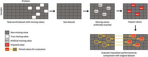
Visualization of the experimental workflow. We first remove all proteins in the real-world dataset that contain at least one MV, creating a “subset data” with no missing values. We then artificially insert missing values into the subset data. The imputed values generated by MVI methods are then compared to the original values to evaluate their accuracy using multiple evaluation metrics.
MCAR- and MNAR-combined MVs are generated as follows: in the |$N\ast M$| dataset, |$N$| denotes samples and |$M$| denotes features (proteins), |$a$| is the proportion of missingness due to MCAR and |$b$| is the proportion of missingness due to MNAR. First, we introduce MNAR by replacing all values in each sample that are below the |$b$|th quantile with ‘Not Available’ (NA). Then, we generate MCAR by randomly choosing |$N\ast M\ast a\ast \left(1-b\right)$| number of values inside the remaining data and replace them with NA. Rows with only NA values are deleted.
To generate a combination of MAR and MNAR in the dataset, we first create MNAR values using the process described above. Next, we generate MAR, where γ represents the proportion of missingness due to MAR. To do this, we randomly select a set of proteins per class and drop values only within the selected proteins. For example, in a |$N\ast M$| dataset of multiple classes with |$n$| samples each, we randomly choose a different set of |$m$| proteins for each class and drop |$n\ast M\ast \gamma \ast \left(1-b\right)$| number of proteins among these |$m\ast n$| proteins.
We inject a total missingness |$\left(a+b\right)$| for MCAR/MNAR missingness and |$\left(\gamma +b\right)$| for MAR/MNAR from 10 to 40%. Inside the total missingness, |$a$| or γ is assigned from 0 to 100% of total missingness with increments of 20% (0, 20, 40, 60, 80 and 100%). For example, if the total missingness is 10%, then |$a$| or γ would be 0, 2, 4, 6, 8 and 10%, respectively. The imputed values are then evaluated against the original values using multiple MVI methods.
Performance evaluation
Normalized root mean square error
To evaluate imputation performance, the normalized root mean square error (NRMSE) is used. NRMSE is a common method for evaluating similarity between the real and imputed data while minimizing the impact of sample variation.
The RMSE is the sum of squares of mean error between each feature of the real dataset |${S}_{ij}$| and imputed dataset |${O}_{ij}$|. The NRMSE is calculated by dividing the standard deviation of RMSE between samples in the real dataset. The formula is shown below:
Procrustes sum of squared error
Procrustes is a method for comparing the consistency of two sets of data by analyzing the shape distribution. Unlike NRMSE, which calculates the error directly, Procrustes transform the data to make the comparison more objective and reasonable. It translates, rotates and scales the imputed data while minimizing the sum of squared difference with the original data matrix. First, dimension-reduction algorithms, such as PCA, partial least squares discriminant analysis or linear discriminant analysis, are introduced to select top components for both datasets [27, 28]. Then, based on the top components, the Procrustes analysis is performed. Finally, the sum of squared difference (SS) is calculated between the estimated and original datasets as a measurement of similarity. Smaller Procrustes SS indicates better imputed outcome. We used the vegan package implementation for Procrustes analysis. The sum of squared error is adapted for evaluation.
Correlation coefficient
Finally, to examine relationship consistency, as a proxy for data integrity, we calculate the Pearson correlation coefficient (r) for all proteins in the real-world dataset against the same set of proteins in the imputed dataset [29]. Higher correlation coefficient suggests the imputation provided an outcome that more closely resembles real-world data.
Functional analysis
For datasets with two classes, we may perform comparative analysis. Welch’s t-test is performed between two classes to identify differential features (e.g. proteins or genes). This is repeated for both original and imputed datasets with P-values adjusted using Benjamini–Hochberg correction [10]. In the original dataset, features with P-value smaller than 0.05 and logFC larger than 1 are named as original-positive (|$P$|), and the remaining features are called original-negative (|$N$|). Similarly, in the imputed dataset, features with P-values smaller than 0.05 are called impute-positive (|${P}^{\prime }$|) and features with P-values larger than 0.05 are called impute-negative (|${N}^{\prime }$|) [30]. The true positive (|$TP$|), false positive (|$FP$|), true negative (|$TN$|) and false negative (|$FN$|) can be derived as shown below.
| Original-positive (|$P$|) | Original-negative (|$N$|) | |
|---|---|---|
| Impute-positive (|${P}^{\prime }$|) | |$TP=\mid{P}^{\prime}\cap P\mid$| | |$FP=\mid{P}^{\prime}\cap N\mid$| |
| Impute-negative (|${N}^{\prime }$|) | |$FN=\mid{N}^{\prime}\cap P\mid$| | |$TN=\mid{N}^{\prime}\cap N\mid$| |
| Original-positive (|$P$|) | Original-negative (|$N$|) | |
|---|---|---|
| Impute-positive (|${P}^{\prime }$|) | |$TP=\mid{P}^{\prime}\cap P\mid$| | |$FP=\mid{P}^{\prime}\cap N\mid$| |
| Impute-negative (|${N}^{\prime }$|) | |$FN=\mid{N}^{\prime}\cap P\mid$| | |$TN=\mid{N}^{\prime}\cap N\mid$| |
| Original-positive (|$P$|) | Original-negative (|$N$|) | |
|---|---|---|
| Impute-positive (|${P}^{\prime }$|) | |$TP=\mid{P}^{\prime}\cap P\mid$| | |$FP=\mid{P}^{\prime}\cap N\mid$| |
| Impute-negative (|${N}^{\prime }$|) | |$FN=\mid{N}^{\prime}\cap P\mid$| | |$TN=\mid{N}^{\prime}\cap N\mid$| |
| Original-positive (|$P$|) | Original-negative (|$N$|) | |
|---|---|---|
| Impute-positive (|${P}^{\prime }$|) | |$TP=\mid{P}^{\prime}\cap P\mid$| | |$FP=\mid{P}^{\prime}\cap N\mid$| |
| Impute-negative (|${N}^{\prime }$|) | |$FN=\mid{N}^{\prime}\cap P\mid$| | |$TN=\mid{N}^{\prime}\cap N\mid$| |
Based on this, we can obtain specificity and sensitivity using the below formula:
The positive and negative classes are often imbalanced in real-world data. This renders traditional standards such as accuracy and F1-score unfeasible as they are affected by imbalanced issues [31]. Hence, we elect to use the geometric mean (GM) of sensitivity and specificity instead.
RESULTS
ProJect provides stable yet accurate imputation performance across all kinds of missingness
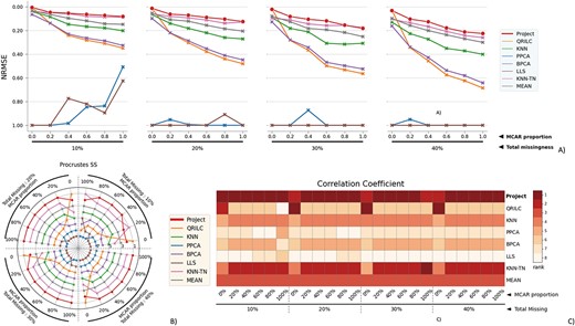
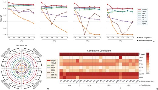
To assess ProJect’s performance on datasets with small sample sizes, we conduct experiments using the OC dataset, which comprises nine samples. Figure 3 provides a visual comparison of the performance of all methods across a range of conditions in the OC dataset. The figure shows how each method performs on accuracy and consistency. ProJect, represented by the red dot, consistently outperforms all other methods (or at minimum, ranks among the top).
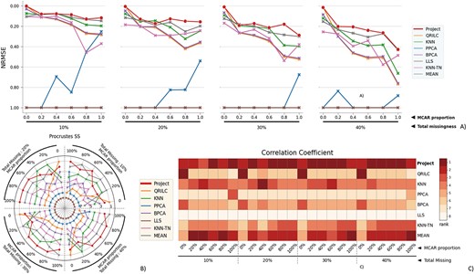
The performance evaluation of 8 different MVI methods on the OC dataset. The figure is divided into 4 blocks, each block representing a different missingness range from 10% to 40%, with missingness being combined of MNAR and MCAR. The x-axis in each block indicates the proportion of MCAR within the combination. The three subfigures within each block provide different perspectives on the performance of the MVI methods. A) The NRMSE score across all combinations, with a lower score indicating a smaller error. For better comparison, the y-axis is labeled from 1.00 at the bottom to 0.00 at the top, so that the better-performing methods are displayed at the top of the chart. B) The rank of Procrustes SS across all combinations, with a smaller rank indicating better performance. The rank is numbered from 1 to 8. C) The heatmap of the rank of the Correlation coefficient, with the darker color indicating a smaller rank. The Correlation coefficient measures the similarity between two datasets, and a smaller rank indicates a better performance of the MVI method in terms of preserving the original relationship between the variables in the data.
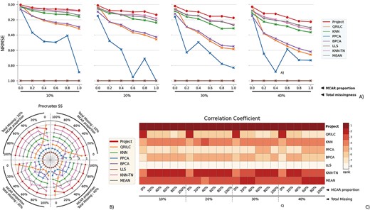
The performance evaluation of 8 different MVI methods on the RC cancer (RC_C) dataset. The figure is divided into 4 blocks, each block representing a different missingness range from 10% to 40%, with missingness being combined of MNAR and MCAR. The x-axis in each block indicates the proportion of MCAR within the combination. The three subfigures within each block provide different perspectives on the performance of the MVI methods. A) The NRMSE score across all combinations, with a lower score indicating a smaller error. For better comparison, the y-axis is labeled from 1.00 at the bottom to 0.00 at the top, so that the better-performing methods are displayed at the top of the chart. B) The rank of Procrustes SS across all combinations, with a smaller rank indicating better performance. The rank is numbered from 1 to 8. C) The heatmap of the rank of the Correlation coefficient, with the darker color indicating a smaller rank. The Correlation coefficient measures the similarity between two datasets, and a smaller rank indicates a better performance of the MVI method in terms of preserving the original relationship between the variables in the data.
BPCA, PPCA, KNN and LLS are known to be specialized tools against MAR. Yet, we see that in the four purely MAR missing scenarios, ProJect obtained the lowest error and highest correlation coefficient. Compared with QRILC that focuses solely on MNAR, ProJect can match its performance on MNAR. In mixed MV missing scenarios with varying MAR proportions (0.2 to 0.8), ProJect consistently dominates.
Traditional local-similarity approaches, such as KNN, only considers local samples and features, lacking consideration of the dataset’s global structure. Conversely, purely global methods, such as PCA, only focus on dominant features, ignoring local and relevant features near MVs.
ProJect optimally combines both local and global approaches using a two-pronged approach of feature-level (i.e. Model 1) and sample-level (i.e. Model 2) supervised learning. ProJect uses an adaptive dimensionality-reduction process by projecting the feature set iteratively when modeling on the feature level, so as to mitigate overfitting that may happen on data with too-high dimension. Yet, ProJect is not limited by the model obtained after dimension reduction and takes into account the whole sample to build a separate model when dealing with higher weighted samples. This balances the pros and cons of imputation on both approaches. In addition, ProJect uses combination parameters specific to the specific dataset obtained through prediction training, resulting in high adaptability to the training dataset and optimal performance.
ProJect tolerates sample differentiation
Compared with OC, the RC_C dataset is more challenging as it has small sample size, large inter-sample variance and non-normal data distribution. Even so, it is clear that ProJect is generally unaffected by these data problems (Figure 4), showing strong yet stable performance across various MV combinations. Unlike BPCA and PPCA that wrongly assume normality when estimating hyper parameters, ProJect assumes a skewed normal distribution, allowing for accuracy and tolerance of skewness. KNN-based methods like KNN-EU and KNN-TN are also outperformed by ProJect as they rely on accurate neighbor identification, which can be impacted by small sample size and large variance between samples.
To assess the robustness of ProJect, we conducted a sensitivity analysis by introducing artificial outliers into the dataset. We created these outliers by randomly choosing 1% of the samples inside the data and replacing them with extreme or non-extreme outliers (Supplementary Figures 1 and 2). Given the high skewness of the RC dataset, we characterized extreme outliers as 2–3 times the global maximum and non-extreme outliers as 1–1.2 times the global maximum. Despite the presence of a few such cases, ProJect continued to outperform other methods. This proves that even when the dataset included anomalous values, ProJect demonstrated a unique capability to successfully separate and impute without these outliers.
ProJect differs from other MVI methods through its mixed-model approach. The first model utilizes the regression process where samples are projected onto a single projection plane and the variance between samples is reduced during the process. This approach assists ProJect in effectively handling datasets where, despite a substantial variance between the number of samples, the underlying trends within each sample on the latent space are similar. It also allows ProJect to identify unusual data points, separate them from the rest and then fill in missing or corrupted data with only relevant information. This process ensured the integrity of the data and allowed for more accurate imputation. The second model is more adaptive, determining the number of selected samples based on their explanatory power, which is not a fixed parameter. This method introduces an element of flexibility that is not commonly found in other MVI methods, allowing ProJect to adapt to the specific characteristics of the dataset it is working with.
By combining these two models, ProJect is less dependent on the size of the sample and the distribution of the data. It maintains strong performance even when faced with less-than-ideal data conditions, making it a highly versatile and robust tool for MVI.
ProJect is robust when dealing with datasets containing confounding effects
The RC full dataset contains two classes, normal and cancer tissues, with each class having two technical replicates. When the data are split by technical replicate, a strong batch effect is observed. Similarly, BladderBatch, a widely used genomic microarray dataset used to evaluate batch effects, also contains two classes from three batches that exhibit a noticeable batch effect. For standard MVI methods, the class effect and batch effect can act as major confounding factors that impact imputation accuracy, as they introduce bias within the dataset [32].
Similar to the OC and RC_C datasets, ProJect demonstrates impressive results on the RC full dataset, displaying the smallest errors while maintaining the highest inter-sample correlations across various missingness rates and both combinations of MCAR/MNAR (Figure 5) and MAR/MNAR (Figure 6). The results show that ProJect is capable of effectively handling class and batch effects by self-differentiating classes and determining correlations between samples. ProJect can recognize the closest samples, i.e. those from the same class and batch, and can also leverage information from sub-nearest samples from different batches and even different classes by transforming the data through projection. This ability is particularly evident in scenarios with high missingness rates and pure MAR missingness, where ProJect demonstrates a dominant performance. With 40% pure MAR missing data (Figure 6), the performance of ProJect highlights its strength in utilizing information from samples in different classes and batches to make up for the lacking information in samples from the same class. Other MVI methods, being less stable and robust, result in inferior performance when compared to even the basic MEAN imputation. Our simulation results show that MEAN imputation, which replaces MVs with the average from all other samples for a particular protein, performs poorly without considering class or batch information. MEAN completely ignores any confounding factors and diminishes the sample variance. ProJect accounts for confounding factors and adjusts correspondingly. The regression step in ProJect self-optimizes and adjusts the feature parameters to minimize variance within the data. In addition, the iterative updating of sample weights in ProJect prioritizes samples with minimal influence from bias.
The performance evaluation of 8 different MVI methods on the full RC dataset. The figure is divided into 4 blocks, each block representing a different missingness range from 10% to 40%, with missingness being combined of MNAR and MCAR. The x-axis in each block indicates the proportion of MCAR within the combination. The three subfigures within each block provide different perspectives on the performance of the MVI methods. A) The NRMSE score across all combinations, with a lower score indicating a smaller error. For better comparison, the y-axis is labeled from 1.00 at the bottom to 0.00 at the top, so that the better-performing methods are displayed at the top of the chart. B) The rank of Procrustes SS across all combinations, with a smaller rank indicating better performance. The rank is numbered from 1 to 8. C) The heatmap of the rank of the Correlation coefficient, with the darker color indicating a smaller rank. The Correlation coefficient measures the similarity between two datasets, and a smaller rank indicates a better performance of the MVI method in terms of preserving the original relationship between the variables in the data.
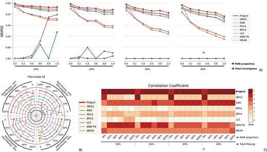
The performance evaluation of 8 different MVI methods on the full RC dataset. The figure is divided into 4 blocks, each block representing a different missingness range from 10% to 40%, with missingness being combined of MNAR and MAR. The x-axis in each block indicates the proportion of MAR within the combination. The three subfigures within each block provide different perspectives on the performance of the MVI methods. A) The NRMSE score across all combinations, with a lower score indicating a smaller error. For better comparison, the y-axis is labeled from 1.00 at the bottom to 0.00 at the top, so that the better-performing methods are displayed at the top of the chart. B) The rank of Procrustes SS across all combinations, with a smaller rank indicating better performance. The rank is numbered from 1 to 8. C) The heatmap of the rank of the Correlation coefficient, with the darker color indicating a smaller rank. The Correlation coefficient measures the similarity between two datasets, and a smaller rank indicates a better performance of the MVI method in terms of preserving the original relationship between the variables in the data.
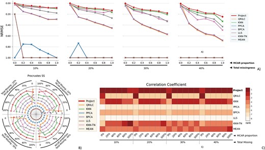
The performance evaluation of 8 different MVI methods on the BladderBatch dataset. The figure is divided into 4 blocks, each block representing a different missingness range from 10% to 40%, with missingness being combined of MNAR and MCAR. The x-axis in each block indicates the proportion of MCAR within the combination. The three subfigures within each block provide different perspectives on the performance of the MVI methods. A) The NRMSE score across all combinations, with a lower score indicating a smaller error. For better comparison, the y-axis is labeled from 1.00 at the bottom to 0.00 at the top, so that the better-performing methods are displayed at the top of the chart. B) The rank of Procrustes SS across all combinations, with a smaller rank indicating better performance. The rank is numbered from 1 to 8. C) The heatmap of the rank of the Correlation coefficient, with the darker color indicating a smaller rank. The Correlation coefficient measures the similarity between two datasets, and a smaller rank indicates a better performance of the MVI method in terms of preserving the original relationship between the variables in the data.
ProJect’s performance extends beyond proteomics data, as evidenced by its impressive results on the BladderBatch dataset, which is commonly used for benchmarking batch effect in genomic data (Figures 7 and 8). However, it is noteworthy to consider the comparative performance of other techniques, such as KNN and KNN-TN. Despite these models relying on unsupervised learning, utilizing automated clustering to differentiate information, they exhibit less proficiency in discerning truly pertinent information when imputing class-specific variables.
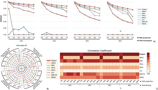
The performance evaluation of 8 different MVI methods on the BladderBatch dataset. The figure is divided into 4 blocks, each block representing a different missingness range from 10% to 40%, with missingness being combined of MNAR and MAR. The x-axis in each block indicates the proportion of MAR within the combination. The three subfigures within each block provide different perspectives on the performance of the MVI methods. A) The NRMSE score across all combinations, with a lower score indicating a smaller error. For better comparison, the y-axis is labeled from 1.00 at the bottom to 0.00 at the top, so that the better-performing methods are displayed at the top of the chart. B) The rank of Procrustes SS across all combinations, with a smaller rank indicating better performance. The rank is numbered from 1 to 8. C) The heatmap of the rank of the Correlation coefficient, with the darker color indicating a smaller rank. The Correlation coefficient measures the similarity between two datasets, and a smaller rank indicates a better performance of the MVI method in terms of preserving the original relationship between the variables in the data.
Similar outcomes are evident with the GBM microarray dataset. Despite its complexity and small size (comprising only seven samples across three classes), the task of imputation is challenging due to the lack of adequate class reference information. Nevertheless, ProJect consistently proves to be the most effective method (Figure 9). KNN-TN has demonstrated commendable results, securing the second position in terms of performance. However, it is worth noting that ProJect still outshines it, reinforcing ProJect’s supremacy in dealing with diverse data sources.
The performance evaluation of 8 different MVI methods on the GBM dataset. The figure is divided into 4 blocks, each block representing a different missingness range from 10% to 40%, with missingness being combined of MNAR and MCAR. The x-axis in each block indicates the proportion of MCAR within the combination. The three subfigures within each block provide different perspectives on the performance of the MVI methods. A) The NRMSE score across all combinations, with a lower score indicating a smaller error. For better comparison, the y-axis is labeled from 1.00 at the bottom to 0.00 at the top, so that the better-performing methods are displayed at the top of the chart. B) The rank of Procrustes SS across all combinations, with a smaller rank indicating better performance. The rank is numbered from 1 to 8. C) The heatmap of the rank of the Correlation coefficient, with the darker color indicating a smaller rank. The Correlation coefficient measures the similarity between two datasets, and a smaller rank indicates a better performance of the MVI method in terms of preserving the original relationship between the variables in the data.
Conversely, it is intriguing to observe that other models, despite their theoretical advantage of discovering inherent patterns in data, have underperformed when dealing with the GBM dataset. In fact, they have shown results that are even inferior to the simple MEAN method. This further underlines the robustness of ProJect and its ability to adapt effectively to different data types and structures. The advantage of ProJect lies in its superior ability to handle complex data and its enhanced precision in extracting useful information, making it highly versatile and effective.
Taken together, the results demonstrate ProJect’s unique strengths, even in the face of challenges such as small sample size, high dimensionality, skewed distribution and unavoidable confounding factors. Unlike other methods that make direct assumptions, ProJect uses a mixed-model optimization approach and trains its parameters, allowing it to effectively adapt to the unique characteristics of the data and maintain robustness, making it a highly reliable algorithm.
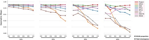
Geometric mean of the 8 methods on simulated RC dataset. For clearer observations, the numbers are log transformed and scaled.

Geometric mean of the 8 methods on BladderBatch dataset. For clearer observations, the numbers are log transformed and scaled.
ProJect preserves the most functional perspective inside the dataset
Like batch-effect correction, MVI also can affect data integrity. Earlier, we used correlation as a rough indicator of data integrity being maintained if the mutual correlations between samples/biological features are retained. Another approach involves conducting a differential analysis and assessing whether the selected genes or proteins are relevant to the phenotypes under comparisons.
To overcome the lack of prior knowledge on differential proteins, we simulate using the RC normal dataset. We create a simulated dataset, referred to as the ‘known set’, containing six normal and six cancer samples. To simulate positive proteins (differentially expressed proteins) inside the cancer samples, we multiply the original expression levels with a random number from a truncated normal distribution. The number of positive and negative proteins is controlled as 1:1 and is chosen randomly. Then, MVs are introduced into the dataset and imputed. The performance of the imputation is evaluated using the GM score.
The GM score of the simulated RC dataset (Figure 10) indicates that ProJect excels in preserving the original biological patterns, thus ranking among the top-performing methods. However, when the missing rate is high and the MAR rate is low, ProJect’s performance is slightly weaker. This may be due to the assumption of a truncated normal distribution in the simulation, which does not accurately reflect the actual shape of the data, particularly for values with low abundance.
The BladderBatch dataset, which contains both cancer and normal microarray data and which has been widely studied, is used to further assess ProJect’s ability to maintain original information. Figure 11 shows that although the GM score decreases slightly with increasing total missing rate, ProJect remains the best and most reliable method for preserving the original features. Other methods, including some sophisticated ones, were unable to retain the biological information. This highlights the effectiveness of ProJect to maintain the original biological features.
DISCUSSION
ProJect is a highly effective MVI method. Its performance is consistent across various datasets that cover diverse high-throughput platforms and evaluation criteria. Despite its versatility in handling MCAR, MAR and MNAR patterns, it still achieves satisfactory results with missing rates as high as 40%. This is attributed to its sophisticated mixed-model approach and adaptable parameter adjustment during training, allowing it to maintain a high tolerance to the inherent characteristics of the data.
Based on the previous result, we found that KNN-TN is the second-best performing method in most cases. However, when compared with ProJect, it exhibits less stability and accuracy. Upon further examination of the sensitivity analysis performance for these two methods, it reveals that ProJect demonstrates a significantly smaller increase in error when outliers are introduced from one sample to two samples (as seen in Supplementary Figures 4 and 5). To understand why ProJect outperforms KNN-TN, we need to delve into the principles behind both methods.
ProJect employs an optimal regression approach for imputation, focusing on the set of correlated features. This approach allows for a more targeted and potentially accurate imputation since it capitalizes on existing relationships within the data. By using only the correlated features, ProJect minimizes the impact of noise or less relevant data points, enhancing the quality of imputation. In addition, ProJect incorporates information from the weighted sample. This strategy lends itself to further improving the accuracy of imputation, as it considers the local data structure around the missing data points. It essentially borrows information from surrounding information, which are likely to be similar due to the spatial correlation in the data.
In contrast, KNN-TN focuses on estimating MVs by identifying similarities in complete data items, without discarding unrelated patterns or outliers. This approach might lead to less precise imputations, particularly in complex datasets where discerning useful subsets and understanding inherent relationships within the dataset play a crucial role.
Furthermore, KNN-TN, by design, assumes that data are truncated normally distributed, an assumption that may not hold true in many real-world datasets. On the other hand, ProJect’s approach does not rely on such assumptions, making it a more versatile tool that can handle a wider variety of data types and distributions.
KNN, similar to what we have discussed, also faces the same issue. It does not discard unrelated patterns or outliers and operates under the assumption of normally distributed data, which is not always the case. Unlike ProJect, KNN does not utilize correlated features specifically or consider the local data structure around missing data points, potentially leading to less accurate imputation.
PPCA is a statistical technique that treats missing data as random variables. It then uses EM to estimate these random variables. This method assumes that both the observed data and the missing data are normally distributed. Similarly, BPCA incorporates a Bayesian framework where it uses prior distributions for parameters and computes a posterior normal distribution, which may not be a valid assumption in real-world scenarios. Furthermore, PPCA and BPCA do not have a built-in mechanism to effectively deal with outliers. Outliers can significantly distort the imputation process, leading to inaccurate results. Unlike PPCA and BPCA, ProJect does not rely on the normality assumption and has mechanisms in place to mitigate the impact of outliers, thus leading to more robust imputation.
LLS performs generally the worst in our benchmark datasets. This method constructs a local linear regression model for each MV using complete data entries, and then fills the MV with the prediction from this local model. However, in high-dimensional datasets like ours, this approach can lead to overfitting, where the model becomes too attuned to the training data and fails to generalize well. Furthermore, the inclusion of noisy or irrelevant features can negatively impact the quality of the imputation. In contrast, ProJect takes a more selective approach to imputation by focusing exclusively on a set of correlated features. This specificity enables ProJect to better capture the underlying data structure, thereby minimizing the impact of less relevant features or noise. This approach results in more robust and accurate imputations, even in high-dimensional datasets.
The MEAN imputation method was ranked top 4 popular MVI method based on published literature [1]. Although widely used, one of the most significant drawbacks is that it tends to underestimate the variability in the data. Consequently, MEAN imputation can skew results in downstream analyses, particularly those that depend on data variance. This method struggles particularly with datasets that include class effects, as evidenced by its subpar performance with GBM, RC full and BladderBatch data. Due to the same reason, MEAN does not perform well when dealing with non-normally distributed data or in the presence of outliers, as proven in the sensitivity analysis. This is because MEAN is sensitive to extreme values, so if the data have outliers, the mean value might not be representative of the underlying data distribution.
Another major limitation is that MEAN does not provide real biological information. It merely fills in the gaps in the data without considering the possible biological implications of the MVs. This lack of biological context can lead to misleading conclusions in downstream analyses, particularly when studying complex biological systems where MVs may have significant implications.
In comparison, methods like ProJect that focus on the correlations between features and consider the local data structure can provide more meaningful and biologically relevant imputations, leading to more robust and accurate downstream analyses.
Lastly, the QRILC method is specifically designed as a pure MNAR imputation approach. It establishes the distribution of complete data by employing the quantile regression model and then uses this inferred normal distribution to impute the MVs. MNAR frequently arises in proteomics, where proteins of low abundance might not be detected. Some studies suggest that methods like QRILC, which handle left-censored data, are particularly suitable for proteomics data for this very reason [8].
However, it is crucial to acknowledge that real-world data often comprises a mixture of different types of MVs. In proteomics, for instance, MVs can emerge due to a range of factors such as limitations in detection thresholds, variability in sample preparation or experimental errors. This results in a complex mix of MCAR, MAR and MNAR.
Although QRILC might excel when all MVs are MNAR, its performance becomes unsatisfactory when confronted with a mixture of missing types. QRILC does not possess the capability to distinguish between these different types of missingness. Consequently, the application of QRILC might be limited in complex, real-world datasets.
In contrast, ProJect features a parameter that allows users to stipulate that all MVs in the dataset are MNAR. This feature is crucial given that although ProJect is equipped to perform imputation through multiple approaches, it must still predict the nature of missingness for each MV based on the available data.
When the ‘purely MNAR’ parameter is activated, ProJect adjusts its prediction values for MVs that exceed a specific threshold. This adjustment leads to improved accuracy, as illustrated in Supplementary Figure 3. However, it is important to exercise caution when specifying this parameter and only do so after thoroughly understanding the dataset. If there is any doubt that the missingness is purely MNAR, the default parameters should be used.
Although ProJect’s mixed modeling approach significantly enhances its accuracy, it does come with increased computational costs and complexity. The training phase of the method, which is the third step, requires numerous iterations, resulting in extended run times. In future work, we aim to improve ProJect’s computational speed. One approach we are considering is re-implementing the method in a language optimized for better memory usage, such as Scala, which would help mitigate computational demands.
ProJect is particularly adept at handling datasets with biological replicates or similar type clinical tissues. The initial phase of ProJect’s algorithm focuses on extracting relationships between features and samples. Consequently, if the samples are largely independent, the performance of ProJect may be compromised. Moving forward, we plan to enhance the algorithm by further exploiting inter-sample relationships and correlations found in biology. For instance, using reference networks could allow us to incorporate biological reasoning, thereby bolstering the reliability of the missing value imputation results.
CONCLUSIONS
Addressing MVs in high-throughput data is crucial for accurate data analysis and effective model development. We introduce ProJect, a novel mixed-model imputation method, as a powerful and versatile solution for handling MVs in diverse data modalities, including genomics and mass spectrometry-based proteomics. ProJect demonstrates consistent and superior performance as evidenced by its success on various benchmark datasets. ProJect achieves the lowest NRMSE and Procrustes SS, along with the highest correlation coefficient across all MV combinations. One key strength of ProJect is its ability to effectively manage different types of MVs commonly found in real-world data, thus providing versatility not seen in most MVI methods designed for a single type of MV. This adaptability is achieved through the utilization of a decision-making algorithm and targeted imputation strategies tailored to the nature of the MVs, leading to more reliable imputation outcomes. ProJect signifies a major advancement in MVI methodologies, presenting a robust and efficient solution for imputing MVs in high-throughput data across diverse modalities and MV types.
ProJect is effective at imputing missing values in diverse high-throughput data from various modalities, including genomics and mass spectrometry-based proteomics.
ProJect is versatile in handling different types of missing values, including mixture of missing at random, missing completely at random and missing not at random.
ProJect’s sophisticated mixed-model approach and adaptable parameter adjustment during training allow it to maintain a high tolerance to the inherent characteristics of the data.
ProJect achieves consistent outstanding performance across various benchmark datasets and can handle missing rates as high as 40%.
FUNDING
This work is supported in part by a Singapore Ministry of Education tier-2 grant (MOE2019-T2-1-042) and a Singapore Ministry of Education tier-1 grant (RG35/20).
AUTHORS’ CONTRIBUTIONS
W.J.K. implemented the analyses, performed initial drafting of the manuscript and developed the figures. B.W.J.H. helped with the manuscript and in arranging the figures. H.H.H. and L.K.P. helped with figures and revision. Y.W. helped with data collection and initial processing. L.W. and W.W.B.G. conceptualized, supervised, provided critical feedback and co-wrote the manuscript.
Author Biographies
Weijia Kong is a thrid year PhD student at Nanyang Technological University. Her research interest include missing protein identification and recovery.
Bertrand Wong Jern Han is a undergraduate student at Nanyang Technological University. He is now pursuring his PhD at Harvard University. His research interest include proteomics and multi-omic analysis.
Harvard Wai Hann Hui is a graduate student at Nanyang Technological University. His research interests include missing value imputation and batch effect correction.
Lim Kai Peng is a final year student at Nanyang Technological University. His research interests includes batch correction for the analysis of proteomics data.
Yulan Wang is a professor of Metabolomics at Lee Kong Chian School of Medicine, Nanyang Technological University. Her research is focused on metabolomics technological development and applications.
Limsoon Wong is Kwan-Im-Thong-Hood-Cho-Temple Chair Professor in the School of Computing at the National University of Singapore (NUS). He was inducted as a Fellow of the ACM, for his contributions to database theory and computational biology. He currently works mostly on knowledge discovery technologies and their application to biomedicine.
Wilson Wen Bin Goh received his undergraduate training in Life Science from National University of Singapore. He was then awarded a Wellcome Trust Scholarship to pursue an MSc in Bioinformatics and PhD in Computing at Imperial College London. Following an EMBO Fellowship at ETH Zurich and a brief stint in Harvard Medical School, Wilson established the Bio-Data Science and Education (BDSE) laboratory in Nanyang Technological University (NTU). Wilson now straddles between the Lee Kong Chian School of Medicine (LKCMed) and School of Biological Sciences (SBS). He serves the academic community as its Director (PhD Programmes), Director (Biomedical Data Science Graduate Programme, Head (Good Research Practice Office) and the Academic Lead of the Data Science Research Programme.
REFERENCES
Hastie T, Tibshirani R, Narasimhan B, Chu G
Song J, Yu C.
Author notes
First Author(s): Weijia Kong
