


Abstract
Circular RNA (circRNA) is closely associated with human diseases. Accordingly, identifying the associations between human diseases and circRNA can help in disease prevention, diagnosis and treatment. Traditional methods are time consuming and laborious. Meanwhile, computational models can effectively predict potential circRNA–disease associations (CDAs), but are restricted by limited data, resulting in data with high dimension and imbalance. In this study, we propose a model based on automatically selected meta-path and contrastive learning, called the MPCLCDA model. First, the model constructs a new heterogeneous network based on circRNA similarity, disease similarity and known association, via automatically selected meta-path and obtains the low-dimensional fusion features of nodes via graph convolutional networks. Then, contrastive learning is used to optimize the fusion features further, and obtain the node features that make the distinction between positive and negative samples more evident. Finally, circRNA–disease scores are predicted through a multilayer perceptron. The proposed method is compared with advanced methods on four datasets. The average area under the receiver operating characteristic curve, area under the precision-recall curve and F1 score under 5-fold cross-validation reached 0.9752, 0.9831 and 0.9745, respectively. Simultaneously, case studies on human diseases further prove the predictive ability and application value of this method.
INTRODUCTION
With the development of sequencing technology, non-coding RNA has been proven to have biological functions, such as participating in cell activities and regulating gene expression. As a type of non-coding RNA, circular RNA (circRNA) is more stable in expression than standard linear RNA because of its special closed-loop structure and for being difficult to degrade. Moreover, circRNA can participate in the expression of pathogenic genes by interacting with microRNA and proteins; consequently, circRNA has attracted considerable attention [1]. Numerous studies have shown that circRNA is related to a variety of human diseases, such as cardiovascular diseases, diabetes, Alzheimer’s disease and cancer. For example, CircFndc3b interacts with the RNA-binding protein fused in a sarcoma to regulate the expression and signalling of the vascular endothelial growth factor; moreover, the overexpression of CircFndc3b in cardiac endothelial cells enhances angiogenic activity and reduces cardiomyocyte apoptosis [2]. CircRNA can also serve as a reliable biomarker and pharmacological target because of its high stability and remarkable tissue specificity. For example, has-circ-0137439 is significantly upregulated in bladder cancer samples [3]. Has-circ-0000190 is down regulated in the plasma of patients with gastric cancer [4]. Therefore, the potential association between circRNA and diseases can provide new possibilities for the early detection and subsequent treatment of diseases.
Conducting molecular biology experiments to study the complex regulatory mechanisms of small molecules and diseases results in blindness in the selection of research objects and requires a high cost. Therefore, researchers have proposed a large number of effective computational models to assist in subsequent biological experiments, such as identifying disease-related biomolecules [5–8], discovering drug target genes and intergenic regulatory mechanism [9–14]. Currently available computational models that predict disease-associated circRNA and provide candidates for subsequent experiments can be roughly divided into three categories: network-based, traditional machine learning-based and deep learning-based models. Network-based algorithms can integrate multiple biological information and flexibly choose similarity calculation methods [15–19]. Lei et al. [20] proposed the PWCDA model, which uses the path weighted method in a heterogeneous network constructed by circRNA similarity network, disease similarity network and circRNA–disease association (CDA) network. PWCDA effectively utilizes the topology of heterogeneous networks, but it only captures path information within three steps and uses a naive decay function. Li et al. [21] developed the DWNCPCDA model for predicting CDAs based on DeepWalk and network consensus projection algorithms. DeepWalk can obtain the topological similarity learning node features of a heterogeneous network to a greater extent, and network consistency projection further uses node features to reveal potential associations. However, the model is still limited by the lack of known associations. To address the sparsity problem of heterogeneous networks caused by insufficient known associations, Deng et al. [22] presented the KATZCPDA model. This model solves the problem of association prediction by introducing protein–disease association information to calculate the similarity of nodes in heterogeneous networks. The additional introduced protein information can increase the number of edges in the heterogeneous network, effectively improving the prediction accuracy. Network-based models can achieve good results; however, this type of model cannot effectively predict disease associations without any known associated circRNA. With the widespread use of traditional machine learning methods in bioinformatics [23–25], the problem of CDA prediction has been transformed into solving various optimization models based on known associations and similarities. Ding et al. [26] developed the RWLR model based on random walk and logistic regression to predict CDAs. RWLR uses random walk with restart to obtain the global information of each circRNA. It utilizes the Gene Ontology terms of related genes to calculate the functional similarity of circRNA. RWLR achieves the prediction of new circRNA that has no known association with any disease. However, it cannot predict the association with circRNA of new diseases that do not have any known association with circRNA. For diseases with no or few known associations with circRNA, Lei et al. [27] proposed a model called ICFCDA. This model uses a collaborative filtering algorithm for solving cold-start problems in recommender systems and adds circRNA sequence similarity, circRNA functional annotation semantic similarity and disease functional similarity to obtain reliable recommendation information. Zuo et al. [28] proposed a DMCCDA model based on double matrix completion. The proposed model uses circRNA sequence information and disease semantic information to update the association matrix to alleviate the problem of insufficient known association. The MLCDA method proposed by Wang et al. [29] integrates circRNA sequence information, circRNA functional similarity information, disease MeSH information and disease DO information, and predicts circRNA–disease association score through inductive matrix completion. This method attempts various methods to integrate similarity information and examines the influence of similarity calculation on the performance of the model. The RNMFLP method proposed by Peng et al. [30] uses a robust non-negative matrix factorization to initially predict the association score on the basis of using matrix multiplication to alleviate the impact of false-negative samples and then uses label propagation to obtain the final association score. The traditional machine learning method maps artificially constructed features to the target space to complete classification [31, 32]. However, finding the classification hyperplane based on the input features to separate positive and negative samples in the training data is difficult. Therefore, some models attempted to train classifiers through the features learned via deep learning and then complete the association inference [33–37]. The CNNCDA model [38] early proposed by Wang et al. uses a convolutional neural network to extract the potential features of circRNA–disease fusion descriptors and input them into an extreme learning machine classifier for prediction. Deepthi et al. [39] further developed the AE-RF ensemble method on the basis of unsupervised learning autoencoders and random forests to predict circRNA–disease associations. Niu et al. [40] combined graph autoencoder and variational inference to capture the structural information of association networks; they proposed the GMNN2CD method, which uses the graph Markov neural network for feature inference. The GATCL2CD model proposed by Peng et al. [41] utilizes a multi-head attention mechanism to dynamically aggregate the feature representations of nodes in a graph. Although the existing models achieved good accuracy in predicting potential associations of circRNA–diseases, they are still limited by data noise caused by insufficient known associations and relying too much on known associations. Therefore, we fully exploit the potential multi-hop connection information of the circRNA–disease association network to alleviate the insufficient known associations and reduce the dependence on known associations through semi-supervised learning.
In this work, we proposed a model, called MPCLCDA, on the basis of automatically selected meta-paths and contrastive learning to predict potential CDAs. First, we dynamically select effective multi-hop connections via meta-paths in the circRNA–disease heterogeneous network to fully utilize the known information of circRNA and diseases. This network is constructed by integrating similarity and known associations. We also reduce the feature dimensions of circRNAs and diseases, respectively, to reduce noise in the data. Then, we use CDAs as nodes for building a topological network and a semantic network to further explore the interaction between CDAs. Thereafter, we utilize GCNs to extract node features in the two networks and generate collaborative contrast loss through comparison and optimization. Finally, a multilayer perceptron (MLP) is used to predict whether potential CDAs exist. The proposed model is compared with advanced methods on four datasets. The average area under the receiver operating characteristic curve (AUC), area under the precision-recall curve (AUPR) and F1 score under 5-fold cross-validation (CV) reach 0.9752, 0.9831 and 0.9745, respectively. Case studies on colorectal cancer, gastric cancer and hepatocellular carcinoma further confirmed that the proposed model can effectively screen candidate circRNA for human diseases and help in subsequent biological experiments.
MATERIALS AND METHODS
In this study, a learning framework called MPCLCDA was proposed to predict CDAs. MPCLCDA first learns the representations of circRNA and diseases by using combinations of a graph transformer network [42] and contrastive learning [43], and then, it employs features to train the classification model and yield the final prediction results. As shown in Figure 1, MPCLCDA consists of the following modules:
(i) Identify useful meta-paths and multi-hop connections on integrated similarities and known associations to learn the low-dimensional representations of circRNA and diseases, respectively.
(ii) Construct a topological network and a semantic network. Calculate collaborative comparison loss and optimize node characteristics with the comparison optimization module.
(iii) Predict the association of circRNA with diseases through MLP.
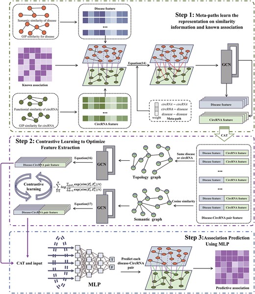
The flowchart of MPCLCD. Step 1, the similarity information and known associations are used to identify useful meta-paths and multi-hop connections to learn representations of circRNAs and diseases, respectively; Step 2, the topological network and semantic network of CDA are constructed, and each node of the two networks is a concatenation of circRNA and disease representation. The node features in the two networks are extracted based on GCN, and the feature extraction is optimized using contrastive learning; Step 3, MLP is used to predict the association between circRNA and disease.
Datasets
To evaluate the performance of the end-to-end heterogeneous graph representation learning-based framework for CDA prediction, we test our model on four benchmark datasets: CircR2Disease [44], circRNADisease [45], Circ2Disease [46] and circAtlas [47]. Four standard datasets are obtained after removing duplicates and non-human disease associations. The CircR2Disease data set collected 650 pairs of associations involving 585 circRNA and 88 diseases. The Circ2Disease data set collected 270 pairs of experimentally validated associations involving 249 circRNA and 59 diseases. The circRNADisease data set collected 310 pairs of experimentally validated associations involving 298 circRNA and 33 diseases. The circAtlas data set collected 930 pairs of experimentally validated associations involving 848 circRNA and 110 diseases. Association matrix A is constructed on the basis of verified associations on the data set, and experiments are performed in the default data set CircR2Disease unless otherwise stated. |${A}_{i,j}=1$| if a verified association exists between circRNA |${c}_i$| and disease |${d}_j$|; |${A}_{i,j}=0$|, otherwise.
Construction of disease similarity
Disease information includes semantic similarity and Gaussian interaction profile (GIP) kernel similarity. The semantic similarity is calculated on the basis of the Diseases Ontology data set, in which diseases are represented as a directed acyclic graph [48]. Then, the semantic similarity between two diseases can be calculated as follows:
where |${N}_{d_i}$| involves |${d}_i$| and its all ancestors, and |${C}_{d_j}(x)$| represents the semantic contribution of disease |$x$| to |${d}_i$|:
where |$\rho$| is the semantic contribution factor, which is assigned as 0.5. However, because of the incomplete annotation, some diseases may be unable to calculate their semantic similarities. In this context, the GIP similarity can be used to supplement the missed disease semantic similarity. The GIP similarity between diseases |${d}_i$|and |${d}_j$| is calculated as follows:
where |$\mathrm{IP}\left({d}_i\right)$| represents the disease interaction profile that corresponds to the ith column of the association matrix A and Nd is the number of diseases. Finally, the disease similarity can be obtained by using the following formula:
Construction of circRNA similarity
CircRNA similarity consists of the circRNA functional similarity and the GIP similarity for circRNA. In accordance with the hypothesis that functionally similar circRNA is associated with the same diseases [49], we calculate the functional similarity through known associations and the disease similarity. In particular, we calculate the functional similarity CFS between circRNA |${c}_i$| and |${c}_j$|.
where |${D}_i$| is the set of diseases associated with |${c}_i$|. |$S\left({d}_p,{D}_i\right)$|represents the similarity between diseases |${d}_p$| and |${D}_i$|. It can be calculated as follows:
Similar to disease, we supplement the data with the GIP similarity for circRNA, which can be calculated as follows:
where |$\mathrm{IP}\left(\bullet \right)$| corresponds to the ith row in the association matrix A and Nc is the number of circRNA. Therefore, the integrated similarity of circRNA can be obtained as follows:
Representation learning based on meta-path
A meta-path is a connecting path composed of multiple types of edges in a heterogeneous network. The potential association formed by different types of edges between objects can be mined using a meta-path [50]. Considering that a CDA network is a heterogeneous network with multiple entities and associations, we use meta-paths to capture its higher-order neighbour information to learn efficient node representations. Simultaneously, to avoid the difficulty of manually designing meta-paths and accurately selecting all meaningful paths, a graph transformer network is used to flexibly select edge types and combination relationships to form meta-paths. Given a set of adjacency matrices |$M=\left\{{M}_1,\cdots, {M}_k\right\}$| (|$k$| is the number of edge types, i.e. circRNA–circRNA, disease–disease and circRNA–disease), new heterogeneous networks are generated using automatically selected meta-paths. In this work, let |$M=\left\{ CS,A, DS\right\}$|. Then, the possible meta-paths are as follows:
where |$A$| is the known association, |$CS$| is the circRNA similarity and |$DS$| is the disease similarity. Then, the weights of each meta-path can be calculated by multiplying |$CS$|, |$DS$| and |$A$|.
To achieve automatic selection of meta-paths, all edge types are trained weights and performed matrix multiplication. Then, a new graph |${M}_{\mathrm{new}}$| of meta-paths is constructed, which consists of two steps:
where |$\bigotimes$| represents the selection of different edge types with weights in |$M$|, and |${W}_l=\left[{\alpha}_1,{\alpha}_2,\cdots, {\alpha}_k\right]$| is the corresponding weight vector. In this manner, different combinations of meta-paths are extracted. Equation (13) generates the new network structure represented by the adjacency matrix obtained through meta-paths, where L combinations are used. The formula is expressed as follows:
where |$k$| is the number of edge types and |${\alpha}_{k_l}^l$| is the weight of edge |${k}_l$| on path length |$l$|.
After obtaining the new meta-path graph, GCN is utilized to learn the feature representations of both disease and circRNA. Afterwards, the feature representation of a circRNA–disease pair can be formed by concatenating these learned representations:
where || represents the catenation operator, |$C$| is the number of meta-paths, |${D}^{-1}$| is the degree matrix of |${M}_{\mathrm{new}}+I$|, |$X$| is the matrix composed of the initial node feature representation and |$W$| is the trainable weight matrix.
Prediction and optimization
Contrastive learning is a self-supervised method that maps similar samples closer and dissimilar samples farther apart [51]. It aims to encode similar samples similarly and make the encoded results of different types of samples as different as possible, for use in similarity-based tasks like classification or clustering. To capture the deep relationships between circRNA and diseases, contrastive learning is used to optimize the feature extraction between circRNA–disease pairs.
Before this process, a topology graph |${H}_t$| and a semantic graph |${H}_s$| should be constructed. In the topology graph, two circRNA–disease pairs (nodes) will be linked if they have the same disease or circRNA. For the semantic graph, the circRNA–disease pair (node) will be linked with its k most similar nodes by calculating the cosine similarity. Finally, two GCNs are respectively used to learn the node features from the topology and semantic graphs:
where |$\overset{\sim }{H}=H+I$|, |$I$| is an identity matrix, |${D}_t$| is the diagonal degree matrix of |${H}_t+I$| and |$W$| is the weight matrix of GCN.
For node |$i$| in the topology graph, node |$j$| from the same node in the semantic graph and node |$j$|’s directly related neighbours are selected as positive samples, whereas the others are regarded as negative samples. InfoCNE divides noise samples into multiple categories and computes the loss between sample features based on their similarity. Contrastive loss, which is calculated using InfoNCE, is utilized to enhance prediction consistency and amplify the dissimilarity between positive and negative samples. It is expressed as follows:
where N is the number of nodes, |${P}_i$| is the set of all positive samples in the semantic graph corresponding to node |$i$| and |$\tau$| is an adjustable scalar parameter.
The features extracted by the nodes in the topological graph and the semantic graph are concatenated and inputted into the MLP to predict whether an association exists between circRNA and disease. MLP can leverage data labels to optimize the model performance and the cross-entropy function is used to calculate the classification loss. The formula of the cross-entropy loss function is as follows:
where |${y}_i$| represents the label of sample |$i$| and |${P}_i$| represents the predicted association probability of the sample. The final loss function is defined as follows:
where |${L}_{cl}$| is the loss function for contrastive learning and |${L}_m$| is the classification loss computed using the cross-entropy function. |$\lambda$| is a hyperparameter between 0 and 1 for balancing the ratio between contrastive and classification losses. |$\Omega (w)$| is the L2 regularization of the parameters to prevent the model from overfitting.
RESULTS
In this section, we used 5-fold CV to compare MPCLCDA with other advanced models on multiple datasets to prove that the proposed model exhibits superior performance. For the model, we analyzed the parameters to find the optimal parameter set, tested the effects of different classifiers on prediction performance and conducted ablation experiments to prove the rationality of the model design. Finally, case studies further demonstrated the validity of the model prediction. In the experiment, we adopted evaluation metrics that are commonly used in machine learning, namely, accuracy (Acc), sensitivity (Sen), precision (Pre), F1 score (F1), AUC and AUPR:
where TP, FP, TN and FN denote the numbers of true positives, false positives, true negatives and false negatives, respectively.
Benchmarking
We chose five other methods, namely, RNMFLP [30], DMCCDA [28], MLCDA [29], AE-RF [39] and GMNN2CD [40], to conduct 5-fold CV comparison on multiple datasets, respectively. To make the experimental results more convincing, we obtained similar results on the CircR2Disease data set and then conducted experiments on the other data sets.
On the CircR2Disease data set, the AUC of MPCLCDA, RNMFLP, DMCCDA, MLCDA, AE-RF and GMNN2CD under 5-fold CV was 0.9877, 0.9512, 0.9615, 0.8619, 0.9514 and 0.9531, respectively. The detailed results are presented in Table 1. MPCLCDA had the highest AUC, which was 2.67% higher than the second place (DMCCDA). Given the extremely small proportion of known CDAs, all unknown associations were used as negative samples in some comparison methods, and accurately judging the effect of the algorithm without sample balance was difficult for Acc. Pre was only slightly lower than that of the GMNNN2CD model, indicating that MPCLCDA exhibited good ability to predict potential CDAs. Although Acc, Sen and Pre did not reach their highest values, they reached the highest values in three levels of indicators (AUC, AUPR and F1), indicating that the model achieved the overall optimal result. That is, it can accurately infer potential associations whilst correctly judging the no association condition.
The performance of different methods on CircR2Disease
| Methods | AUC | AUPR | F1 | Acc | Sen | Pre |
|---|---|---|---|---|---|---|
| MPCLCDA | 0.9877 | 0.9892 | 0.9878 | 0.9876 | 0.9954 | 0.9806 |
| RNMFLP | 0.9512 | 0.2194 | 0.3779 | 0.9753 | 0.5954 | 0.2768 |
| DMCCDA | 0.9615 | 0.7351 | 0.7016 | 0.9920 | 0.5599 | 0.9393 |
| MLCDA | 0.8619 | 0.0373 | 0.1388 | 0.8433 | 1.0000 | 0.0746 |
| AE-RF | 0.9514 | 0.9692 | 0.9177 | 0.9196 | 0.9317 | 0.9043 |
| GMNN2CD | 0.9531 | 0.6717 | 0.6985 | 0.9941 | 0.5394 | 0.9907 |
Note: The highest value for each metric is shown in bold.
To further prove the superiority of the proposed model, we compared it with other methods on the Circ2Disease, circRNADisease and circAtlas datasets. The AUC values obtained under 5-fold CV are listed in Table 2. DMCCDA failed to converge with the default parameters on the Circ2Disease and circRNADisease datasets. The two datasets were not used in their study, and thus, we changed some parameters of the model to obtain results. As indicated in Table 2, MPCLCDA could perform well on all datasets, and it achieved the highest AUC on three datasets, and only slightly lower than that of DMCCDA on the circRNADisease data set. Although MPCLCDA was less effective than DMCCDA on the circRNADisease data set, its performance on circAtlas was considerably better than that of DMCCDA, indicating that our model demonstrated better adaptability and generalization ability for an increase in the number of circRNA and diseases. GMNN2CD also achieved good results in the four datasets, but they were all weaker than MPCLCDA. In addition, the paired t-test is utilized to measure the statistical differences between MPCLCDA and other methods, and the results are documented in Table 3. The results show that the effect size of the MPLCDA method compared with other methods, as measured by Cohen value, was >0.8, indicating a large difference between the methods. Through the preceding analysis, a conclusion could be drawn that MPCLCDA can predict disease-related circRNA more accurately than other advanced methods on multiple data sets.
The AUC of different methods on four data sets
| Dataset | MPCLCDA | RNMFLP | DMCCDA | MLCDA | AE-RF | GMNN2CD |
|---|---|---|---|---|---|---|
| CircR2Disease | 0.9877 | 0.9512 | 0.9615 | 0.8619 | 0.9514 | 0.9531 |
| Circ2Disease | 0.9799 | 0.8852 | 0.9700 | 0.8204 | 0.9497 | 0.9343 |
| circRNADisease | 0.9743 | 0.9329 | 0.9878 | 0.8053 | 0.9655 | 0.9735 |
| circAtlas | 0.9587 | 0.8012 | 0.8267 | 0.8006 | 0.8489 | 0.9532 |
Note: The highest value for each metric is shown in bold.
Measurement of the statistical differences between MPCLCDA and other methods
| MPCLCDA VS | RNMFLP | DMCCDA | AE-RF | GMNN2CD | MLCDA |
|---|---|---|---|---|---|
| Mean difference | 0.080 | 0.040 | 0.050 | 0.020 | 0.150 |
| t-value | 2.921 | 1.202 | 2.105 | 1.976 | 16.259 |
| P-value | 0.061 | 0.316 | 0.126 | 0.143 | 0.001 |
| Cohen’s value | 1.460 | 0.601 | 1.053 | 0.988 | 8.129 |
Finally, to demonstrate the excellence of our method comprehensively, we present the performance comparison of all methods on all four datasets in Table 4. AUC, AUPR and F1 were mostly used for evaluation, and the bold text in the table indicates the optimal performance of this metric in the dataset. Our method outperforms the majority of other methods across all datasets.
Comparison of AUC, AUPR and F1 of different methods on four data sets
| Data set | Metrics | MPCLCDA | RNMFLP | DMCCDA | MLCDA | AE-RF | GMNN2CD |
|---|---|---|---|---|---|---|---|
| CircR2Disease | AUC | 0.9877 | 0.9512 | 0.9615 | 0.8619 | 0.9514 | 0.9531 |
| AUPR | 0.9892 | 0.2194 | 0.7351 | 0.0373 | 0.9690 | 0.6761 | |
| F1 | 0.9878 | 0.3779 | 0.7016 | 0.1388 | 0.9177 | 0.6985 | |
| Circ2Disease | AUC | 0.9799 | 0.8852 | 0.9700 | 0.8204 | 0.9497 | 0.9343 |
| AUPR | 0.9830 | 0.1418 | 0.7564 | 0.0743 | 0.9569 | 0.7394 | |
| F1 | 0.9799 | 0.2730 | 0.7982 | 0.2584 | 0.8854 | 0.7665 | |
| circRNADisease | AUC | 0.9743 | 0.9329 | 0.9878 | 0.8053 | 0.9655 | 0.9735 |
| AUPR | 0.9851 | 0.3281 | 0.9265 | 0.0446 | 0.9791 | 0.8891 | |
| F1 | 0.9736 | 0.42 | 0.8967 | 0.1638 | 0.9163 | 0.8889 | |
| circAtlas | AUC | 0.9587 | 0.8012 | 0.8267 | 0.8006 | 0.8489 | 0.9532 |
| AUPR | 0.9787 | 0.0903 | 0.1745 | 0.0395 | 0.8608 | 0.6943 | |
| F1 | 0.9568 | 0.1651 | 0.1863 | 0.1466 | 0.7811 | 0.6576 |
Note: The highest value for each metric is shown in bold.
Performance analysis of MPCLCDA
The MPCLCDA model has several parameters. By analyzing its parameters, the optimal parameter set is found to maximize the potential of the model. In the following sections, we discuss the meta-path length |$l$|, the number of channels |$C$|, the feature dimension |$d$| extracted by the meta-path and the balance loss parameter |$\lambda$|. Meanwhile, as the major parts of MPCLCDA, meta-path and contrastive learning play key roles. We also observe the performance of the model by removing them in turn to understand their roles accurately. Finally, we test different existing classifiers to verify the effect of using MLP as the final choice in the current study.
Parameter analysis
In this section, we analyze the effects of model parameters on performance. Parameter |$l$| in Equation (14) represents the length of the meta-path adopted in the model. The length of each path increases correspondingly as the value of |$l$| increases. The influence of the change in length |$l$| on each index is depicted in Figure 2. In Equation (15), |$C$| controls the number of distinct meta-paths used in the model. Selected different |$C$| experimental results are presented in Figure 3. The larger the parameter value, the more time and computing resources are consumed. When the values of |$l$| and |$C$| are >2, the model will only change slightly. Therefore, |$l$| = 2 and |$C$| = 2. The influence of the feature dimension |$d$| extracted by the meta-path on the performance of the model is shown in Figure 4. The results show that the model achieves better results as the dimension increases and the model achieves the highest AUC value when the dimension is 128, so the parameter |$d=128$|. Given that the data label and the similarity between data are used to optimize the performance and learning ability of the model, the value of |$\lambda$| in the loss function balances comparison and classification losses, we sequentially select from (1, 0.5, 0.1, 0.05, 0.01). In accordance with the experimental results in Figure 5, when |$\lambda$| = 0.1, the balance between losses is optimal.
Comparison of meta-path length l = 1, 2, 3.

Comparison of meta-path channels C = 1, 2, 3, 4.
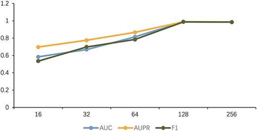
Comparison of dimension d = 16, 32, 64, 128, 256.
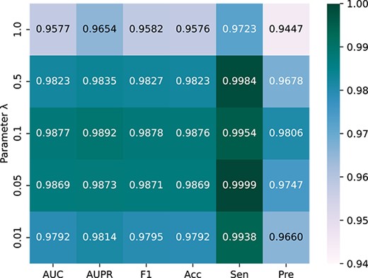
Comparison of parameter λ on model performance.
By adjusting the learning rate (0.005, 0.001, 0.0005, 0.0001, 0.00005, 0.00001), in turn, a more accurate prediction ability of the model is achieved. As shown in Figure 6, the learning rate is 0.0005, which is the highest value of various indicators of the model. To prove the stability of the model, Figure 7 presents the change trend of loss with an increase in epoch during the experiment. When the epoch is 200, the loss tends to be stable, and the model is converged when the epoch reaches 300. We finally adopt this set of optimal parameters |$l$| = 2, |$C$| = 2 and |$\lambda$| = 0.1. We iterate 300 times at a learning rate of 0.0005. In addition, we conducted experiments using different proportions of known associations and the results are shown in Figure 8. When the known correlation exceeds 60%, the model can achieve good results above 0.9 under multiple indicators. Only when the known correlation accounts for 20%, the model performance drops greatly. Therefore, it can be inferred that our model is not sensitive to known correlations.
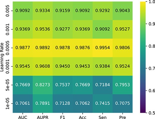
Performance comparison with different learning rates.
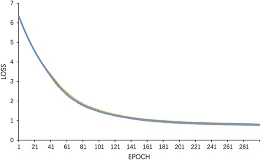
Loss curve of MPCLCDA model.
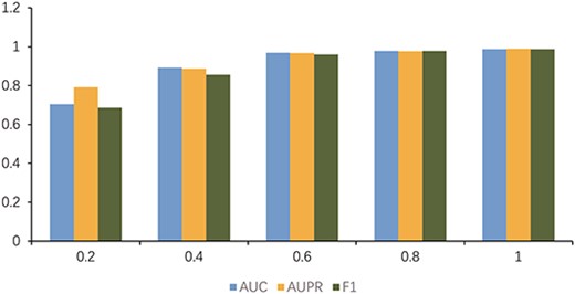
The impact of the proportion of known associations on MPCLCDA.
Ablation experiment
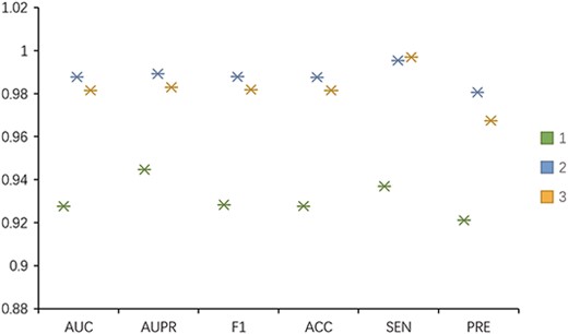
To trace the influences of meta-path and contrastive learning in the model on performance, we remove the parts of meta-path and contrastive learning in turn and conduct 5-fold CV on the CircR2Disease data set to observe the effect on performance under multiple indicators. By removing the meta-path part, we directly use the similarity and known association as the features of nodes for contrastive learning. Then, we use an MLP to obtain the classification results. Without using contrastive learning, the features extracted by the meta-path are concatenated as associated features and inputted into the MLP to obtain the prediction results. The experimental results are presented in Figure 9. The combination of meta-path and contrastive learning is 8% higher than that without meta-path and 4% higher than that without contrastive learning. The meta-path can obtain potentially effective multi-hop connections between circRNA and diseases. It can learn node features in an end-to-end manner to alleviate noise in the data. Contrastive learning can take circRNA–disease as a whole and further learn the interaction between associations by taking advantage of similarities existing amongst associations. From the preceding discussion, the combination of meta-path and contrastive learning is reasonable and can more effectively predict potential association of circRNA with diseases.
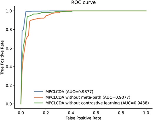
The performance of MPCLCDA, MPCLCDA without meta-path and MPCLCDA without contrastive learning in terms of AUC.
Influences of different classifiers
To verify the influence of the classifier on the prediction ability of the model, we compare MLP with five commonly used classifiers, namely, support vector machine (SVM), random forest (RF), naive Bayes (NB), decision tree (DT) and gradient boost (GB), via 5-fold CV on the CircR2Disease data set. The five classification algorithms are taken from the sklearn library. The parameter probability of the SVM classifier is set to True, and the number of DTs in the RF classifier is 100. The NB classifier adopts the BernoulliNB class, which is suitable for the sample feature to be binary discrete value. We finally achieve the best average AUC values of MLP, SVM, RF, NB, DT and GB, which were 0.9877, 0.8646, 0.9715, 0.7646, 0.8992 and 0.9477, respectively. The experimental results are presented in Figure 10. In the figure, the MLP classifier achieves the highest values amongst all the indicators. Although the RF classifier can achieve similar good results, it requires more computing resources as a method of ensemble learning. The NB classifier performs poorly because of the large attribute correlation between CDAs. Thus, MLP is more suitable for the classification of this model.
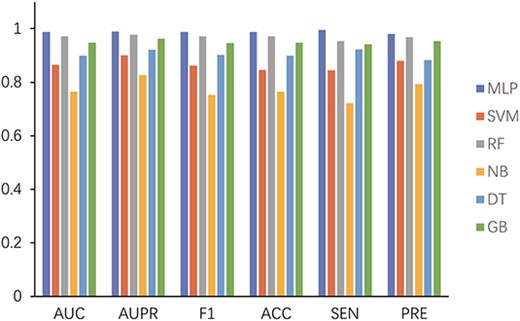
Performance comparison of different classifiers for the MPCLCDA model.
Case study
To demonstrate the model’s ability to predict potential associations, we trained it with all the known associations, and then used it to predict unknown association scores between specific diseases and circRNAs. Finally, in accordance with the predicted probability ranking, we selected the top 10 associated circRNA of three diseases (colorectal cancer, gastric cancer and hepatocellular carcinoma) and verified them by searching the literature in PubMed.
Colorectal cancer is a cancer with high morbidity and mortality, and it remains completely curable. As a common type of cancer, gastric cancer has no evident early symptoms and is less likely to be cured when it develops to an advanced stage. Hepatocellular carcinoma is the most common cause of death amongst patients with cirrhosis, accounting for 90% of liver cancer cases. Therefore, studying these disease-associated circRNA as potential biomarkers is extremely valuable. As indicated in Table 5, at least seven of the top 10 circRNA predicted for these diseases have been documented in the literature. For example, the overexpression of has-circ-0005927 can inhibit the formation of colorectal cancer cells and induce apoptosis; this finding provides a theoretical basis for the targeted therapy of colorectal cancer [52]. CircNOL10 mediates colorectal cancer cell cycle by sponging miR-135a-5p and miR-135b-5p [53]. The expression level of has-circ-0004872 correlates with tumour size and local lymph node metastasis; it forms a negative regulatory loop that consists of has-circ-0004872/miR-224/Smad4/ADAR1 in gastric cancer [54]. P53 and p21, two key cellular senescence regulators, are elevated in cicrLARP4-overexpressed hepatocellular carcinoma cells [55]. Although no literature proves that circ-104916 regulates hepatocellular carcinoma, studies have shown that the expression of circ-104916 is downregulated in gastric cancer tissues [56]. Considering that circRNA CDR1as exerts an effect on the proliferation and migration of hepatocellular carcinoma and gastric cancer cells, circ-104916 may be potentially associated with hepatocellular carcinoma [57, 58]. We conducted a literature search on PubMed to further validate the top 30 predicted circRNA–disease pairs with the highest scores, and the results of this search are documented in Supplementary File (Table S2) of the article for reference and further analysis. Case studies demonstrate the model’s ability to contribute to the understanding of disease mechanisms and provide potential therapeutic candidates.
The top 10 associations identified by MPCLCDA for colorectal cancer, gastric cancer and hepatocellular carcinoma
| Cancer | CircRNA | Evidence |
|---|---|---|
| Colorectal cancer | has-circ-0005927 | PMID: 33732022 |
| circNOL10 | PMID: 32606737 | |
| has-circ-0005075 | PMID: 31476947 | |
| circFAT1 | PMID: 34257702 | |
| has-circ-0035431 | Unconfirmed | |
| circRHOBTB3 | PMID: 34158864 | |
| circ-FBXW7 | PMID: 31519156 | |
| has-circ-0058246 | Unconfirmed | |
| hsa-circRNA-103809 | PMID: 30249393 | |
| hsa-circ-0001821 | PMID: 34298612 | |
| Gastric cancer | hsa-circ-0004872 | PMID: 33172486 |
| has-circ-0000673 | PMID: 35833385 | |
| circ-SHKBP1 | PMID: 32600329 | |
| has-circ-0000064 | PMID: 34245111 | |
| has-circ-0000615 | PMID: 31773689 | |
| has-circ-0067934 | PMID: 35475447 | |
| has-circ-0005015 | Unconfirmed | |
| has-circ-0066922 | Unconfirmed | |
| has-circ-0006988 | PMID: 35975639 | |
| has-circ-0081108 | Unconfirmed | |
| Hepatocellular carcinoma | circLARP4 | PMID: 30520539 |
| has-circ-0085616 | PMID: 31496798 | |
| circ-104916 | Unconfirmed | |
| has-circ-101889 | PMID: 35080329 | |
| has-circRNA-104348 | PMID: 33311442 | |
| has-circ-0015756 | PMID: 32884351 | |
| has-circRNA-103809 | PMID: 32683589 | |
| has-circ-0058246 | Unconfirmed | |
| has-circ-0078710 | PMID: 34139933 | |
| has-circ-0035431 | Unconfirmed |
CONCLUSION
Numerous studies have shown that circRNA can be used as disease biomarkers to guide the prevention, diagnosis and treatment of human diseases [4, 58]. However, the performance of the general calculation model cannot be improved because of the high dimension and unbalance of the data. On the basis of an automatic meta-path method and contrastive learning, this study overcomes the two aforementioned difficulties through multiple extractions of node features. The MPCLCDA model is proposed to predict potential associated circRNA of diseases, providing candidate circRNA for subsequent biological experiment verification. First, we extract latent features of circRNA and diseases in the integrated similarity matrix and known association matrix by automatically selecting meta-paths, respectively. Then, regard CDA as a whole to construct a topological graph and a semantic graph and optimize node feature extraction in the two graphs through contrastive learning. Finally, we use MLP to predict whether CDA exists. The ablation experiment proves the rationality of the model design. The average AUC, AUPR and F1 scores under 5-fold CV on multiple datasets reach 0.9752, 0.9831 and 0.9745, respectively, indicating that MPCLCDA can stably and accurately predict disease-related circRNA. Comparison with other advanced methods on different datasets shows that MPCLCDA has more accurate prediction ability. The case studies further validate the ability of MPCLCDA to predict the potential association of circRNA with diseases.
The reasons for the superior performance of this model are as follows. (i) MPCLCDA effectively explores the multi-hop potential connection between circRNA and disease by automatically selecting meta-paths and learning the feature representation of diseases and circRNA in an end-to-end manner, alleviating data noise. (ii) On the basis of the features extracted from the meta-paths, each association is used as a node to construct a hypergraph. A semantic similarity graph is constructed via cosine similarity, and the interaction between associations is further mined using contrastive learning. (iii) The losses of contrastive learning and classification are integrated to fully utilize data labels and the similarity between CDAs to optimize the performance of the model in a semi-supervised manner.
Although the model can effectively predict CDAs, some limitations still exist. First, the model has several parameters, and the acquisition of suitable parameters requires multiple experiments. Second, the model relies on known associations whilst fully utilizing these associations. At present, known associations are considerably less than unknown associations, affecting the performance of the model. Introducing other biological information to strengthen circRNA and disease similarity or add potential associations may further improve the predictive ability of the model. In addition, circRNA affects diseases by interacting with other small molecules, and thus, introducing interactions between circRNA and other small molecules, predicting circRNA that is potentially associated with diseases and further exploring the pathway of circRNA that affects diseases will help in understanding disease mechanisms.
We propose an MPCLCDA model to predict potential circRNA associated with diseases, providing candidate circRNA for subsequent biological experiment verification.
In MPCLCDA, we explore multi-hop potential connections between circRNA and diseases by automatically selecting meta-paths. Then, we optimize node feature extraction via contrastive learning for circRNA–disease associations as a whole.
Compared with other state-of-the-art methods, MPCLCDA exhibits more accurate prediction ability. The case studies further validate the ability of MPCLCDA to predict potential association of circRNA with diseases.
ACKNOWLEDGEMENTS
The authors would like to thank Xingen Sun for proofreading the manuscript.
FUNDING
The Scientific Research Fund of Hunan Provincial Education Department (Grant Nos 22A0101 and 22A0350).
DATA AVAILABILITY STATEMENT
The code, data and corresponding supplementary materials can be downloaded from https://github.com/XTU-Liu/MPCLCDA.
Author Biographies
Wei Liu is an associate professor at Xiangtan University. His research interest is bioinformatics.
Ting Tang is a graduate student at Xiangtan University. Her research interest is bioinformatics.
Xu Lu is a professor at Guangdong Polytechnic Normal University. His research interest is bioinformatics.
Xiangzheng Fu is a postdoctoral scholar at Hunan University. His research interest is classification of proteins in bioinformatics
Yu Yang is a graduate student at Xiangtan University. His research interest is bioinformatics.
Li Peng is an associate professor at Hunan University of Science and Technology. Her research interest is bioinformatics.
