


Abstract
Multiple sequence alignment is widely used for sequence analysis, such as identifying important sites and phylogenetic analysis. Traditional methods, such as progressive alignment, are time-consuming. To address this issue, we introduce StarTree, a novel method to fast construct a guide tree by combining sequence clustering and hierarchical clustering. Furthermore, we develop a new heuristic similar region detection algorithm using the FM-index and apply the k-banded dynamic program to the profile alignment. We also introduce a win-win alignment algorithm that applies the central star strategy within the clusters to fast the alignment process, then uses the progressive strategy to align the central-aligned profiles, guaranteeing the final alignment's accuracy. We present WMSA 2 based on these improvements and compare the speed and accuracy with other popular methods. The results show that the guide tree made by the StarTree clustering method can lead to better accuracy than that of PartTree while consuming less time and memory than that of UPGMA and mBed methods on datasets with thousands of sequences. During the alignment of simulated data sets, WMSA 2 can consume less time and memory while ranking at the top of Q and TC scores. The WMSA 2 is still better at the time, and memory efficiency on the real datasets and ranks at the top on the average sum of pairs score. For the alignment of 1 million SARS-CoV-2 genomes, the win-win mode of WMSA 2 significantly decreased the consumption time than the former version. The source code and data are available at https://github.com/malabz/WMSA2.
INTRODUCTION
Multiple sequence alignment (MSA) is critical in various aspects of sequence analyses, such as the function and structure prediction of nucleotide sequences, identification of conserved regions, and phylogenetic reconstruction. However, the problem of finding an optimal MSA based on the sum of pairs (SP) score is NP-complete. Currently, most MSA tools, including FMAlign [1], MAFFT [2], CLUSTAL [3], MUSCLE [4], Kalign3 [5], T-Coffee [6], HAlign3 [7] and WMSA [8], are heuristic or approximate methods. There are three main approaches: progressive, central star and combined central-progressive alignment. Furthermore, iterative alignment on the preliminary alignment result can correct the gap errors by repeatedly realigning parts of sequences [9].
Progressive and iterative methods first need to build a guide tree, where each leaf represents a sequence to be aligned. The guide tree determines the sequence alignment order; the most similar sequences must be aligned first. The usual way to construct a guide tree is hierarchical clustering, such as the UPGMA [10] and neighbor-joining [11] algorithm with quadratic [12] or cubic time complexity. However, most alignments adopt an approximate algorithm to compute the distance matrix, which may reduce the accuracy of alignment: such as PartTree in MAFFT [13], mBed in CLUSTALΩ [14], and FastTree2 [15], which lower the time complexity but sacrifice accuracy.
The profile-profile alignment in progressive strategy also requires |$O\left({m}_1{m}_2{L}_1{L}_2\right)$| (|$m$| is the length of the profile, and |$L$| is the number of sequences in the profile) time. Some aligners, such as MAFFT [2], PASTA [16], and MAGUS [17], use the divide-and-conquer algorithm, split the sequences/profile into segments, align each subset individually, then merge them together to speed up the profile-profile alignment. However, MAFFT cannot align large datasets, PASTA is limited to medium and small datasets due to limited memory and time [18], and MAGUS can only align datasets with a maximum of 40 000 sequences [19].
Center star alignment is a simplified tree alignment, which aligns fast without profile-profile alignment, but alignment performance is not good on low-similarity datasets [20]. HAlign [7, 21, 22] is a multiple sequence alignment software that uses the center star alignment method to align ultra-large numbers of similar DNA/RNA datasets. Furthermore, WMSA [8] is the first tool to combine progressive and center star alignment reducing computing time complexity and space on large, highly similar sequences. The main idea of WMSA is divide-and-conquer using clustering. First, WMSA clusters the dataset by modified CD-HIT; Second, each cluster is aligned by a center star method; Last, profiles are aligned by the progressive alignment method using the FFT/K-Band alignment algorithm. Compared with MAFFT, WMSA reduces the alignment time but sacrifices the alignment's accuracy.
In this paper, we presented a fast method WMSA 2 for multiple sequence alignment based on sequence clustering and the full-text index in minute space (FM-index) [23] that accelerates the construction of the guide tree and profile alignment. We first developed CluStar, a new fast-clustering method based on heuristic clustering and sequence length restriction, which can cluster the sequences with similar lengths and high similarity into clusters that would get the best alignment results. By combining CluStar and UPGMA, we proposed StarTree, which generates the main branches of the guide tree through the center sequences in each cluster, creates a subtree for each cluster, then merges the main branches with all subtrees to obtain a final guide tree. For pairwise sequence alignment (PSA) and profile-profile alignment, we first converted the profile into a consensus sequence, then used the FM-index to search for common substrings between two (consensus) sequences to divide the dynamic program (DP) and align the rest part of sequences by k-banded DP [20], which significantly reduce the complexity of the alignment, especially in similar sequences. In the win-win mode, WMSA 2 combines the central and progressive alignment strategies, applies the central alignment within the StarTree clusters to speed up the alignment, then uses FM-index/k-banded DP to progressively align the central-aligned profiles, which immensely fastens the alignment speed while also guaranteeing the high alignment accuracy for big data sets.
METHOD
CluStar
CluStar is based on a heuristic sequence cluster method combining sequence length information and the similarity of sequences, which is the number of matches divided by the alignment length. For the similarity threshold of clustering, five thresholds (0.8\0.85\0.9\0.95\0.99) were tested on the simulated RNA datasets shown in Table 1. The results show that with the increase of similarity threshold, the time and memory of alignment will increase, but the alignment accuracy is not necessarily improved. And the similarity of 0.9 is better than other thresholds in the TC score, shown in Table 2. In the Q score, 0.9, 0.95 and 0.99 are better than 0.8 and 0.85 and they all have close scores. Therefore, we chose 0.9 as the default parameter of the similarity threshold, which reduces the alignment memory and time and guarantees alignment accuracy. Two sequences whose length difference is greater than 10% must have a similarity of lower than 0.9. Therefore, the default parameter of the length clustering threshold is set to 10% accordingly, indicating that the sequences with a length difference of less than 10% would be assigned to the same cluster. The details of the algorithm are shown in Algorithm 1.
CluStar for sequence clustering
| Input: nucleotide sequences Output: clusters |${c}_j\ \left(j\ge 1\right)$| 1. Divide the sequences with length difference less than 10% into one block |${B}_i\left(i\ge 1\right)$| 2. Align each block using center star alignment (used to compute the sequence similarities fast and accurately) 3. For each block |${B}_i$| a. Pick the longest sequence in the block |${B}_i$| b. Compute the similarities between the longest and remaining sequences in the block |${B}_i$|. c. Pick the sequences for which the similarity is greater than the threshold of 0.9. These sequences and the longest one form a new cluster |${c}_j$|. d. If the block |${B}_i$| is not empty, return to step a. 4. All blocks are done. Obtain the clusters |${c}_j\ \left(j\ge 1\right)$|. |
| Input: nucleotide sequences Output: clusters |${c}_j\ \left(j\ge 1\right)$| 1. Divide the sequences with length difference less than 10% into one block |${B}_i\left(i\ge 1\right)$| 2. Align each block using center star alignment (used to compute the sequence similarities fast and accurately) 3. For each block |${B}_i$| a. Pick the longest sequence in the block |${B}_i$| b. Compute the similarities between the longest and remaining sequences in the block |${B}_i$|. c. Pick the sequences for which the similarity is greater than the threshold of 0.9. These sequences and the longest one form a new cluster |${c}_j$|. d. If the block |${B}_i$| is not empty, return to step a. 4. All blocks are done. Obtain the clusters |${c}_j\ \left(j\ge 1\right)$|. |
The summary of datasets
| Dataset | Number | Number of the repeat sets | Average length | Min length | Max length |
|---|---|---|---|---|---|
| Simulation RNA | 255 | 10 | 1527 | 1518 | 1542 |
| 511 | 1528 | 1518 | 1542 | ||
| 1023 | 1527 | 1517 | 1542 | ||
| 2047 | 1527 | 1517 | 1542 | ||
| 4095 | 1527 | 1516 | 1542 | ||
| 8191 | 1527 | 1514 | 1542 | ||
| SARS-CoV-2-like simulated genomes with various mean similarities (90%–99%) | 100 | 9 | 29 837 ± 114 | 29 650 ± 237 | 29 996 ± 5 |
| SARS-CoV-2-like simulated genomes with varying scales of tree length (0.05–15) | 29 675 ± 178 | 29 404 ± 316 | 30 000 ± 0 | ||
| Mitochondrial-like simulated genomes with various mean similarities (90%–99%) | 15 860 ± 115 | 15 719 ± 220 | 15 992 ± 12 | ||
| Mitochondrial-like simulated genomes with varying scales of tree length (0.05–5) | 15 840 ± 87 | 15 675 ± 169 | 16 000 ± 3 | ||
| Ancient human partial mitochondrial DNA | 393 | \ | 372 | 341 | 413 |
| SARS-CoV-2 genome | 1020 | \ | 27 656 | 64 | 29 981 |
| 1000000 | 29 774 | 21 111 | 29 891 |
Suppose there are 𝑛 nucleotide sequences with an average length of 𝑚. In that case, the time complexity of the clustering is |$O\left[n\left( km+{p}_2\right)\right]$| (the higher the similarity of the sequences in one cluster is, the lower |$k$| is; |$k$| is the width of banded dynamic programming, the same as the following; |${p}_1$| is the number of clusters after sequence clustering; |${p}_2$| is the number of clusters after similarity clustering and |${p}_1\le{p}_2$|): Step 1 in Algorithm 1 requires |$O\left(n{p}_1\right)$| time; Step 2 involves |$O(kmn)$| time since there will be |$n$| pairwise sequence alignments whose time complexity is |$O(km)$| (see more details in 2.4 profile-profile alignment); Step 3 has a time complexity of |$O\left(n{p}_2\right)$| time. The central alignments in blocks |${B}_i$| result in higher time complexity but guarantee more reliable clustering.
StarTree
Inspired by the idea of divide and conquer, we developed a new method to build the guide tree by combining CluStar and the UPGMA. The algorithm details are shown in Algorithm 2 and Figure 1A (WMSA 2 progressive mode). If there are |$ n. $| nucleotide sequences with an average length of |$ m $|, the time complexity of building the guide tree is |$ O\left[n\left( km+{p}_2+n/{p}_2\right)\right] $|, which includes the time complexity of CluStar clustering and UPGMA. The time complexity of UPGMA is |$ O\left(\frac{n^2}{p_2}+{p}_2^2\right) $|.
StarTree for building the guide tree
| Input: nucleotide sequences |$S$| Output: a guide tee |$T$| |${c}_j/{t}_j$|represents the cluster/subtree belonging to cluster |$j$|. 1. Cluster the sequences |$S$| using the CluStar method. Obtain the clusters |${c}_j\ \left(j\ge 1\right)$|. 2. For each |${c}_j$|, build a UPGMA subtree |${t}_j$|. 3. Pick the central sequence (the longest one) in each cluster |${c}_j$|, form a new |${S}^{\prime }$|, and build a main branch of the guide tree |${t}^{\prime }$|. 4. Merge the main branch |${t}^{\prime }$| with all subtrees |${t}_j$| to obtain the final guide tree |$T$|. |
| Input: nucleotide sequences |$S$| Output: a guide tee |$T$| |${c}_j/{t}_j$|represents the cluster/subtree belonging to cluster |$j$|. 1. Cluster the sequences |$S$| using the CluStar method. Obtain the clusters |${c}_j\ \left(j\ge 1\right)$|. 2. For each |${c}_j$|, build a UPGMA subtree |${t}_j$|. 3. Pick the central sequence (the longest one) in each cluster |${c}_j$|, form a new |${S}^{\prime }$|, and build a main branch of the guide tree |${t}^{\prime }$|. 4. Merge the main branch |${t}^{\prime }$| with all subtrees |${t}_j$| to obtain the final guide tree |$T$|. |
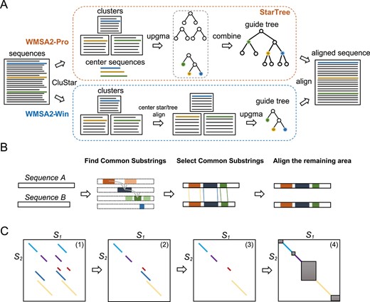
Algorithm diagram of WMSA2. (A) The main procedure of progressive and win-win modes of WMSA 2, and the StarTree algorithm is shown in the orange dash box. (B) The primary process of PSA. The four sets of colored fragments in the second panel represent the total common substrings of sequences A and B. The dashed bar represents the position of sequence A, which together with fragments indicated the location of common substrings accordingly. (C) An example of selecting the common substrings. (1) All common substrings found in |${S}_1$| and |${S}_2$|; (2) when one common substring in |${S}_2$| corresponds to several regions in |${S}_1$| (colored substrings), select the substrings with smaller location offset; (3) use DP to search for the longest and non-overlapped substrings, which filter out the blue string; (4) delete the substrings (red) with a larger offset than its length to filter out possible short tandem repeat. The dark area is ready to be aligned by k-banded DP.
Pairwise sequence alignment
Based on the Burrows–Wheeler transform, FM-index can compress and index the full-text substring by taking up much less space than the suffix array. Therefore, FM-index is first applied to find the common substrings between two sequences to be aligned (Figure 1B). After finding all common substrings (longer than 1% of the length of in |${S}_2$|), the following three situations may occur: one common substring in |${S}_2$| corresponds to several regions in |${S}_1$|, different common substrings in |${S}_2$| overlap in |${S}_1$|, and common substrings have a large location offset. We solve these three problems in three steps: (1) filter out the substrings with bigger location offset when one common substring in |${S}_2$| corresponds to several regions in |${S}_1$|; (2) use DP to search for the longest and non-overlapped substrings combination; (3) delete the substrings with a larger offset than its length to filter out possible short tandem repeat (Figure 1C). The final optimized common substring pairs can be used as part of the alignment result, which saves DP time and memory complexity. The rest substring pairs are individually aligned by k-banded dynamic programming [20], as shown in Algorithm 3.
PSA with FM-index
| Input: nucleotide sequences |${S}_1\ \mathrm{and}\ {S}_2$| Output: aligned sequences |$S{\prime}_1\ \mathrm{and}\ S{\prime}_2$| Assume |$\mathrm{length}\left({S}_1\right)\ge \mathrm{length}\left({S}_2\right)$| 1. Build the FM-index for |${S}_1$|. 2. While |$i< len\left({S}_2\right)$|, |$i$| starts at 1. Begin index |$i$| in |${S}_2$| to find the longest common substrings |$lc{s}_j$| in |${S}_1$|. i + = len(lcsj) 3. The selection of optimized longest and non-overlapped common substring combinations. 4. Align the optimized common substrings directly, and use k-banded DP to align the remaining segments individually. Join segments and common substrings. Return the aligned sequences |$S{\prime}_1\ \mathrm{and}\ S{\prime}_2$|. |
| Input: nucleotide sequences |${S}_1\ \mathrm{and}\ {S}_2$| Output: aligned sequences |$S{\prime}_1\ \mathrm{and}\ S{\prime}_2$| Assume |$\mathrm{length}\left({S}_1\right)\ge \mathrm{length}\left({S}_2\right)$| 1. Build the FM-index for |${S}_1$|. 2. While |$i< len\left({S}_2\right)$|, |$i$| starts at 1. Begin index |$i$| in |${S}_2$| to find the longest common substrings |$lc{s}_j$| in |${S}_1$|. i + = len(lcsj) 3. The selection of optimized longest and non-overlapped common substring combinations. 4. Align the optimized common substrings directly, and use k-banded DP to align the remaining segments individually. Join segments and common substrings. Return the aligned sequences |$S{\prime}_1\ \mathrm{and}\ S{\prime}_2$|. |
The DP in WMSA 2 uses affine gap penalties, which usually require three matrices of size |$\left({m}_1+1\right)\left({m}_2+1\right)$| (|$m$| is the sequence length) to store the score and also increase the space consumption. Here instead, WMSA 2 uses three matrices of size |$\left({m}_1+1\right)$| to only store the current DP scores and an additional matrix size |$\left({m}_1+1\right)\left({m}_2+1\right)$| to store all the state transitions, adapted from Kalign 3. Once the state transition was recorded, the three matrices of size |$\left({m}_1+1\right)$| can be renewed with the DP score of the next state.
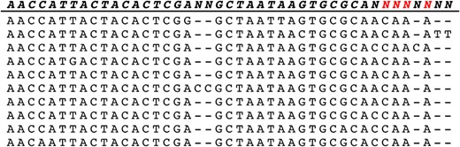
Modified consensus sequence. ‘N’ in red were modified sites.
Building the FM-index requires |$O\left(m\log m\right)$| time in step 1. Steps 2 and 3 have linear time complexity. The time complexity of step 4 mainly comes from the k-banded dynamic programming. Since in most cases, |$O\left(m\log m\right)\ll O(kq)$|, thus, the time complexity of PSA in WMSA 2 is equal to |$O(kq)$| which is the time complexity of the alignment of the longest segment (|$k$| represents the bandwidth, and |$q$| represents the longest segment length). Our method can significantly reduce PSA's time and memory costs for similar sequences compared to general dynamic programming; for dissimilar sequences, it still saves space for improving the DP score storing.
Profile-profile alignment
Profile-profile alignment is more complicated than sequence alignment since all sites become a one-dimensional vector instead of one value, which causes the FM-index to be inapplicable. Therefore, it is impossible to find identical segments between profiles directly. In WMSA 2, by taking advantage of the idea of consensus sequence, we transform the profile into a modified consensus sequence based on the consistency and continuity of columns. For example, in Figure 2, the bases (A/T/C/G) whose percentage is greater than 90% in a given column will be shown in the consensus sequence; otherwise, it will be recorded as the character ‘N’. Then, only keep the bases (A/T/C/G) that consecutively occur at more than 15 sites; otherwise, the bases will be modified into the character ‘N’. Thus, similar to the PSA above, profile-profile alignment can benefit from the FM-index and k-banded DP methods, as shown in Algorithm 4, which will dramatically lower the time complexity in similar sequences.
Profile alignment with FM-index
| Input: nucleotide profiles |${P}_1\ \mathrm{and}\ {P}_2$| Output: aligned profiles |${P}_{a1}\ \mathrm{and}\ {P}_{a2}$| Assume |$len\left({P}_1\right)\ge len\left({P}_2\right)$| 1. Simplify |${P}_1\ \mathrm{and}\ {P}_2$| as two modified consensus sequences |${S}_1\ \mathrm{and}\ {S}_2$|. 2. Build the FM-index for |${S}_1$|. 3. While |$i< len\left({S}_2\right)$|, |$i$| starts at 1. Begin index |$i$| in |${S}_2$| to find the longest common substrings |$lc{s}_j$| in |${S}_1$|. i + = len(lcsj) 4. The selection of optimized longest and non-overlapped common substring combinations. 5. Directly align the profile region relative to the optimized common substrings, and use k-banded DP to align the remaining profile segments individually. Join all aligned segments together to return the aligned profiles |${P}_{a1}\ \mathrm{and}\ {P}_{a2}$| |
| Input: nucleotide profiles |${P}_1\ \mathrm{and}\ {P}_2$| Output: aligned profiles |${P}_{a1}\ \mathrm{and}\ {P}_{a2}$| Assume |$len\left({P}_1\right)\ge len\left({P}_2\right)$| 1. Simplify |${P}_1\ \mathrm{and}\ {P}_2$| as two modified consensus sequences |${S}_1\ \mathrm{and}\ {S}_2$|. 2. Build the FM-index for |${S}_1$|. 3. While |$i< len\left({S}_2\right)$|, |$i$| starts at 1. Begin index |$i$| in |${S}_2$| to find the longest common substrings |$lc{s}_j$| in |${S}_1$|. i + = len(lcsj) 4. The selection of optimized longest and non-overlapped common substring combinations. 5. Directly align the profile region relative to the optimized common substrings, and use k-banded DP to align the remaining profile segments individually. Join all aligned segments together to return the aligned profiles |${P}_{a1}\ \mathrm{and}\ {P}_{a2}$| |
Progressive and win-win modes of WMSA 2
Although we optimize the construction of the guide tree and profile alignment, which significantly reduces the time complexity, facing ultra-large datasets requires a high time cost due to the increased time complexity of progressive alignment. Therefore, we develop a win-win heuristic method for ultra-large datasets by combining center star and progressive alignment. As shown in Figure 1A, the WMSA2-Pro represents the progressive alignment mode, which depends on the guide tree built by the StarTree algorithm. The WMSA2-Win stands for the win-win mode of combining the center star and progressive alignment that aligns the sequences within the CluStar clusters by the central strategy, then progressively aligns the central-aligned profiles based on the guide tree built from the center sequences of each cluster. WMSA2-Win mode can significantly reduce the computational costs with a slighter decrease in the alignment accuracy, which is sufficiently low and acceptable since sequences in one cluster are highly similar.
RESULTS
We conducted two sets of experiments, including comparing the performance of StarTree with PartTree and mBed and comparing WMSA 2 and other MSA programs, including the previous version of WMSA v0.4.4 [8], FMAlign [1], HAlign v3.0.0_rc1 [7], MAFFT v7.490 [2], ClustalΩ v1.2.4 [3], MUSCLE v3.8.31 [4] and Kalign v3.3.2 [5]. The analyses were implemented on a server with fifty-six 3.5 GHz 4-core CPUs, 512 GB of memory and a 64-bit Ubuntu operating system. We used the Q and TC scores calculated by the MUSCLE Q-Score [4] to evaluate the alignment accuracy for simulated datasets with reference alignment to compare. To evaluate the alignment accuracy of real datasets, we chose the average sum-of-pairs score value, equal to the sum of every pairwise alignment score [21, 22] divided by the number of sequences.
During the comparations, the simulated datasets we used are: (1) an extensive simulation RNA dataset (CIPRES simulation data) [24]. The number of sequences in the simulation RNA dataset ranges from 255 to 8191 (Table 1). (2) Hierarchical tree simulated datasets [7], two sets of SARS-CoV-2-like and two sets of mitochondrial-like genome datasets. We also compared three real datasets: (1) an ancient human partial mitochondrial DNA [25] dataset downloaded from GenBank (https://www.ncbi.nlm.nih.gov/genbank/) under the accession numbers KF600801-KF601193; (2) a small dataset with 1020 SARS-CoV-2 genomes [7, 26], which has a large sequence length variation; (3) an big dataset with 1 million (1 M) SARS-CoV-2 genomes [7]. More specific details are given in Table 1. All datasets can be downloaded from the link in Table 1.
Performance comparison on simulated RNA datasets with a similarity threshold of 0.8, 0.85, 0.9, 0.95 and 0.99
| Datasets | Similarity threshold | Q | TC | Memory (GB) | Time (min) |
|---|---|---|---|---|---|
| RNA-255 | 0.8 | 0.979 | 0.753 | 0.249144 | 0.0865 |
| 0.85 | 0.977 | 0.779 | 0.258788 | 0.083 | |
| 0.9 | 0.979 | 0.77 | 0.292468 | 0.0875 | |
| 0.95 | 0.982 | 0.771 | 0.315456 | 0.098333 | |
| 0.99 | 0.98 | 0.782 | 0.335812 | 0.1 | |
| RNA-511 | 0.8 | 0.928 | 0.541 | 0.449184 | 0.118167 |
| 0.85 | 0.94 | 0.552 | 0.476004 | 0.123167 | |
| 0.9 | 0.941 | 0.576 | 0.525592 | 0.122667 | |
| 0.95 | 0.941 | 0.56 | 0.607832 | 0.128833 | |
| 0.99 | 0.94 | 0.56 | 0.726308 | 0.1355 | |
| RNA-1023 | 0.8 | 0.964 | 0.567 | 0.868212 | 0.155 |
| 0.85 | 0.972 | 0.598 | 0.924364 | 0.1645 | |
| 0.9 | 0.975 | 0.623 | 1.119212 | 0.194 | |
| 0.95 | 0.976 | 0.625 | 1.21642 | 0.187333 | |
| 0.99 | 0.973 | 0.608 | 1.348644 | 0.2015 | |
| RNA-2047 | 0.8 | 0.9 | 0.342 | 1.357644 | 0.255333 |
| 0.85 | 0.891 | 0.349 | 1.35318 | 0.2915 | |
| 0.9 | 0.895 | 0.362 | 1.345952 | 0.336667 | |
| 0.95 | 0.891 | 0.349 | 1.345912 | 0.3605 | |
| 0.99 | 0.889 | 0.347 | 1.34692 | 0.407833 | |
| RNA-4095 | 0.8 | 0.687 | 0.363 | 1.364532 | 0.434333 |
| 0.85 | 0.725 | 0.383 | 1.369564 | 0.575 | |
| 0.9 | 0.763 | 0.409 | 1.407104 | 0.731667 | |
| 0.95 | 0.764 | 0.395 | 1.354636 | 0.868667 | |
| 0.99 | 0.752 | 0.4 | 1.3491 | 1.009 | |
| RNA-8191 | 0.8 | 0.871 | 0.212 | 1.368952 | 1.114833 |
| 0.85 | 0.925 | 0.236 | 1.380232 | 1.691333 | |
| 0.9 | 1.04 | 0.243 | 1.42806 | 2.129333 | |
| 0.95 | 1.08 | 0.243 | 1.36974 | 2.701 | |
| 0.99 | 1.05 | 0.245 | 1.396428 | 3.194333 |
Experiment 1. Compare the performance of StarTree with PartTree and mBed
Traditional methods for building a guide tree, such as the UPGMA, have high time and space complexity for large datasets. Thus, we developed StarTree, a fast method for building a guide tree. We selected two sets of simulated datasets, one with an increasing number of sequences (ranging from 255 to 8191) and the other with distinct sequence similarities (the datasets with tree lengths from 7.5 to 15 have an average sequence similarity from 0.75 to 0.8, the longer the tree length, the lower the similarity). During the comparations, we use UPGMA, StarTree, PartTree and mBed methods to build guide trees, respectively, then progressively align the datasets by the PSA and profile-profile alignment algorithms of WMSA 2, based on these different guide trees. The alignment accuracy, time and space consumption during tree building were compared.
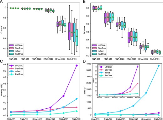
Performance comparison based on simulation RNA Datasets. (A) Comparison of Q scores (mean ± SD). (B) Comparison of TC scores (mean ± SD). (C) Comparison of memory (mean) during guide tree building. (D) Comparison of time (mean) during guide tree building. The inset indicates the zoomed-in results of UPGMA, StarTree and PartTree.
Figure 3 shows that the alignment accuracy based on the four guide trees is close according to the Q and TC scores. But overall, the alignment accuracy of UPGMA and StarTree is higher than the other two methods, and StarTree has an advantage on TC score. UPGMA took much more space than others (Figure 3C). The time taken to build a guide tree with the mBed is much larger than others, and PartTree is the fastest, followed by StarTree (Figure 3D). In the datasets with 4095 and 8191 sequences, UPGMA takes 2–3-folds of time than StarTree. Therefore, StarTree effectively reduces time and space consumption while maintaining alignment accuracy on datasets with thousands of sequences. In the simulated SARS-CoV-2-like genome datasets with relatively lower similarities, the comparison also showed that StarTree has a higher score value than mBed and PartTree, and is very close to UPGMA (Figure S1) while taking similar time and space to UPGMA, since the small number of (100) sequences in each dataset. Thus, StarTree can also maintain high alignment accuracy on datasets with low similarity.
Experiment 2.1. Comparison of WMSA 2 with the other aligners on simulated datasets
In this comparison, we tested all the aligners on four sets of simulated datasets: SARS-CoV-2-like and mitochondrial-like genomes simulated by different gradients of tree length (the longer the tree length is, the similarity is lower) or mean similarity. Except for WMSA 2, default parameters were used for all aligners. The alignment accuracy, consumption time and space were compared, as shown in Figure 4 and Figure S2. Regarding the Q score, MUSCLE is the highest, followed by the WMSA2-Pro and Kalign3, while ClustalΩ and the previous version of WMSA are lower than others. MUSCLE, WMSA2-Pro and Kalign3 have close Q scores (the difference is lower than 0.01). Furthermore, the alignment accuracy of aligners differs in TC score, and WMSA2-Pro has a more significant advantage (Figure 4A and B and Figure S2). The maximum memory usage of the aligners increases when the sequence similarity decreases. However, ClustalΩ, MUSCLE, FMAlign and MAFFT need more memory than WMSA2-Pro, Kalign3, and the previous version of WMSA (Figures 4C and S2). HAlign has a minor time consumption since it only adopts the center star strategy, and WMSA2-Pro takes the minimum time cost except for HAlign (Figures 4D and S2). Therefore, the progressive alignment mode of WMSA 2 ranks at the top of the state-of-art aligner. The Q and TC scores of WMSA2-Win mode are close to MUSCLE, Kalign3, FMAlign, and MAFFT, and higher than HAlign, WMSA and ClustalΩ. The time and memory consumption of WMSA2-Win, slightly less than WMSA2-Pro, ranked at the forefront of nine aligners. It indicates that combining the center star strategy with the progressive strategy sacrificed alignment accuracy while promoting alignment efficiency. Besides, the improvements in time and memory consumption of WMSA2-Win to WMSA2-Pro are not significant, possibly due to the number of sequences of simulated datasets not being big enough to show.
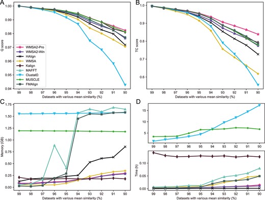
Performance comparison of WMSA 2, HAlign v3.0.0_rc1, WMSA v0.4.4, Kalign v3.3.2, MAFFT v7.490, ClustalΩ v1.2.4, MUSCLE v3.8.31 and FMAlign based on hierarchical tree simulated Mitochondrial-like genome datasets (nine replicates for each dataset with similarity of 99%, 98%, 97%, 96%, 95%, 94%, 93%, 92%, 91% and 90%). (A) Comparison of Q scores (mean ± SD). (B) Comparison of TC scores (mean ± SD). (C) Comparison of alignment memory (mean). (D) Comparison of alignment time (mean).
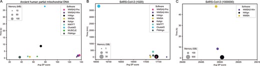
Performance comparison among WMSA 2, HAlign v3.0.0_rc1, WMSA v0.4.4, Kalign v3.3.2, MAFFT v7.490, ClustalΩ v1.2.4, MUSCLE v3.8.31 and FMAlign based on the ancient human partial mitochondrial DNA dataset and SARS-CoV-2 genome datasets. (A) Performance comparison of the eight programs based on the ancient human partial mitochondrial DNA dataset. (B) Performance comparison of the seven programs based on the SARS-CoV-2 (1020) genome dataset, MUSCLE cannot complete the alignment of this dataset. (C) Performance comparison among WMSA2-Win, HAlign and WMSA based on the SARS-CoV-2 (1M) genome dataset; other tools cannot complete the alignment of this dataset.
Experiment 2.2. Comparison of WMSA 2 with the other aligners on real datasets
On the real datasets of mitochondria and SARS-CoV-2 genomes, the average sum-of-pairs score is used to evaluate the alignment accuracy since the absence of reference alignment. WMSA2-Win and WMSA2-Pro modes were used in the comparison, and the other alignment tools were set in their default parameters. As shown in Figure 5, WMSA2-Win and WMSA2-Pro perform well in the two small datasets regarding memory and time cost, and the average sum-of-pairs scores are better than aligners (Figure 5A and B). For the big dataset, which has 1 million SARS-CoV-2 genomes, only WMSA2-Win, former WMSA, and HAlign can complete the alignments (Figure 5C), implying that there are significant time-consuming drawbacks in aligning big data using progressive methods. The consumption time, memory and SP score of WMSA2-Win are improved compared to the former WMSA. With a very close average SP score, WMSA2-Win takes much less space than central strategy representative HAlign and makes the alignment of the big dataset possible in a modified progressive strategy.
DISCUSSION AND CONCLUSION
Among the state-of-the-art tools in the paper, ClustalΩ is a time-consuming multiple sequence alignment tool that cannot align large datasets such as the SARS-CoV-2 (1M) genome. Furthermore, its alignment accuracy is the lowest. MUSCLE also needs to spend more time, but it gets the highest score in Q-score. MAFFT can speed up the alignment of similar sequence datasets because of the divide-and-conquer strategy, such as the SARS-CoV-2 genome. Still, it cannot align the ultra-large SARS-CoV-2 (1M) genome datasets. Kalign has an advantage in memory cost and alignment accuracy but requires more time on large datasets like the SARS-CoV-2 genome. FMAlign is a software based on MAFFT, which can reduce the alignment time in similar sequences but has a lower accuracy than MAFFT in our experiments. HAlign is the fastest software in our experiments and receives a high average sum-of-pairs score in the alignment of SARS-CoV-2 genomes. Still, HAlign consumes much more memory and has a lower Q and TC score in the simulated datasets. The previous version of WMSA is a fast alignment software developed on the alignment tool MAFFT and CD-HIT clustering methods, sacrificing alignment accuracy. WMSA 2 is one of the most rapid tools that can complete the alignment of the big dataset, takes much less space than HAlign (the representative of the center star alignment tool), and achieves high Q and TC scores.
Center star alignment is a particular tree alignment that uses a central sequence to align the remaining sequences. Thus, star alignment has low time complexity since it does not build an approximate guide tree and perform profile alignment. Therefore, it only works with highly similar sequences. On the other hand, progressive alignment is applicable for various sequences but has much higher time complexity. By conducting sequence clustering, sequences in one cluster are highly similar; within a highly similar sequence cluster, applying the center star alignment would probably reduce the time consumption. This work presents WMSA 2, a new multiple nucleotide sequence alignment method with two modes: WMSA2-Pro and WMSA2-Win. Both alignment modes rank at the top compared to their similar tools. WMSA2-Pro employs the standard progressive alignment method to obtain high accuracy; WMSA2-Win, combining the center star and progressive alignment, achieves a better balance between accuracy and efficiency and is more applicable with ultra-large datasets such as SARS-CoV-2 (1M).
StarTree is a fast way to build a guide tree, using sequence similarity and length to cluster datasets to divide and conquer the UPGMA tree build process.
FM-index searching for common substrings, modified consensus sequence, and k-banded DP significantly reduced the calculation complexity on PSA and profile-profile alignment.
The win-win mode of WMSA 2 combines the central and progressive alignment strategies, immensely fastening the alignment speed while guaranteeing high alignment accuracy for big data sets.
FUNDING
National Natural Science Foundation of China (62250028, 62271353, 62102065 and 62001311); Sichuan Provincial Science Fund for Distinguished Young Scholars (2021JDJQ0025); Natural Science Foundation of Sichuan Province (2022NSFSC0926); Municipal Government of Quzhou (2022D020); Joint Funds for the innovation of science and Technology, Fujian province (2022J05055); Fujian Medical University Research Foundation of Talented Scholars (XRCZX2022003).
DATA AVAILABILITY
All test data sets are available on the website (http://lab.malab.cn/soft/WMSA2) and are described in Table 1.
Author Biographies
Juntao Chen is a master student at Quzhou People’s Hospital, Quzhou Affiliated Hospital of Wenzhou Medical University, Quzhou, China, Yangtze Delta Region Institute (Quzhou), University of Electronic Science and Technology of China, Quzhou, China, and the Institute of Fundamental and Frontier Sciences, University of Electronic Science and Technology of China, Chengdu, China.
Jiannan Chao is a master student at Yangtze Delta Region Institute (Quzhou), University of Electronic Science and Technology of China, Quzhou, China, and the Institute of Fundamental and Frontier Sciences, University of Electronic Science and Technology of China, Chengdu, China.
Huan Liu is a research fellow at School of Computer Science and Technology, Southwest University of Science and Technology, Mianyang, China.
Fenglong Yang is an associate professor at Department of Bioinformatics, Fujian Key Laboratory of Medical Bioinformatics, School of Medical Technology and Engineering, Fujian Medical University, Fuzhou, China.
Quan Zou is a professor at Yangtze Delta Region Institute (Quzhou), University of Electronic Science and Technology of China, Quzhou, China and the Institute of Fundamental and Frontier Sciences, University of Electronic Science and Technology of China, Chengdu, China.
Furong Tang is a special associate researcher at Quzhou People’s Hospital, Quzhou Affiliated Hospital of Wenzhou Medical University, Quzhou, China, and Department of Basic Medical Sciences, School of Medicine, Tsinghua University, Beijing, China.
