


Abstract
The discovery of drug–target interactions (DTIs) is a pivotal process in pharmaceutical development. Computational approaches are a promising and efficient alternative to tedious and costly wet-lab experiments for predicting novel DTIs from numerous candidates. Recently, with the availability of abundant heterogeneous biological information from diverse data sources, computational methods have been able to leverage multiple drug and target similarities to boost the performance of DTI prediction. Similarity integration is an effective and flexible strategy to extract crucial information across complementary similarity views, providing a compressed input for any similarity-based DTI prediction model. However, existing similarity integration methods filter and fuse similarities from a global perspective, neglecting the utility of similarity views for each drug and target. In this study, we propose a Fine-Grained Selective similarity integration approach, called FGS, which employs a local interaction consistency-based weight matrix to capture and exploit the importance of similarities at a finer granularity in both similarity selection and combination steps. We evaluate FGS on five DTI prediction datasets under various prediction settings. Experimental results show that our method not only outperforms similarity integration competitors with comparable computational costs, but also achieves better prediction performance than state-of-the-art DTI prediction approaches by collaborating with conventional base models. Furthermore, case studies on the analysis of similarity weights and on the verification of novel predictions confirm the practical ability of FGS.
INTRODUCTION
A crucial step in drug discovery is identifying drug–target interactions (DTIs), which can be reliably conducted via laborious and expensive in vitro experiments. To reduce the expensive workload of the wet-lab based verification procedure, computational approaches are adopted to efficiently filter potential DTIs from a large amount of candidates for subsequent biological experiments [1]. Computational approaches rely on machine learning techniques, such as kernel machines [2], matrix factorization [3], network mining [4] and deep learning [5], to build a prediction model, with the goal of accurately estimating undiscovered interactions based on the chemogenomic space that incorporates both drug and target information.
In the past, the primary information used by computational approaches was the chemical structure of drugs and the protein sequence of targets, from which a single drug and target similarity matrix could be obtained to describe the relationship between drugs and targets in the chemogenomic space [6]. For instance, matrix factorization methods [7, 8] decompose the interaction matrix into latent drug and target feature matrices that preserve the local invariance of entities in the chemogenomic space. WkNNIR [9], a neighborhood method, recovers possible missing interactions of known drugs (targets) and predicts interactions for new entities using proximity information characterized by chemical structure and protein sequence-based similarities. Apart from computing similarities, other solutions to describe characteristics of drug structures and target sequences include utilizing handcrafted molecular fingerprints and protein descriptors [10, 11], as well as learning more robust high-level drug and target representations by graph, recurrent and transformer neural networks [12–14].
With the advancement of biological databases, there is a renewed interest in utilizing various drug and target-related information retrieved from heterogeneous data sources to improve the effectiveness of DTI prediction models. Multiple similarities could be derived and calculated upon diverse types of drug (target) information, assessing the relation between drugs (targets) in complementary aspects. There are two main schemes used by DTI prediction methods to handle multiple similarities: (i) building a prediction model capable of directly processing multiple similarities, and (ii) combining multiple similarities into a fused one, and then learning a prediction model upon the integrated similarities [15–17]. Approaches following the first strategy jointly learn a linear combination of multiple similarities and train a prediction model, which is usually a matrix factorization or kernel-based model [2, 3, 18]. On the other hand, the second strategy can shrink the dimension of input space via the similarity integration procedure, improving the computational efficiency of prediction models. Furthermore, flexibility is another merit of the second strategy, since any similarity integration method and DTI prediction model can be used.
Similarity integration is a crucial step in the second strategy, which determines the importance and reliability of the input similarities for the DTI prediction model, and further influences the accuracy of the predictions. Linear similarity integration methods accumulate multiple similarity matrices, each of which is multiplied by a weight value to indicate the importance of the corresponding similarity view to the DTI prediction task [2, 16, 17, 19]. However, the linear weights are defined according to the whole similarity matrices, failing to distinguish the utility of each similarity view for different entities (drugs or targets). For example, a drug similarity view is useful for drugs sharing the same interactivity in proximity, but is detrimental to others surrounded by neighbors interacting with different targets. Similarity Network Fusion (SNF) [20], a nonlinear integration method, can enhance the relationships between drugs that are proximate in multiple views via inter-view information diffusion. Nevertheless, it completely discards the supervised interaction information. In DTI prediction, SNF usually collaborates with similarity selection to remove noisy and redundant similarity views, but it processes similarity matrices in a global way, neglecting the entity-wise utility [15, 21].
In addition to calculating multiple similarities, another way to deal with multi-source biological information is to construct a heterogeneous DTI network, composed of various types of entities (nodes) and edges. Network-based methods learn topology-preserving representations of drugs and targets via graph embedding approaches to facilitate DTI prediction. However, they usually conduct embedding generation and interaction prediction as two independent tasks, failing to fully exploit supervised interaction information in the embedding generation step [4, 22]. Deep learning models, especially graph neural networks, have also been successfully applied to infer new DTIs from a heterogeneous network due to their capacity to capture complex underlying information [5, 23–25]. Although deep learning models have achieved improved performance, they require larger amounts of training data and are computationally intensive.
This study focuses on the similarity integration approach, which preserves crucial information from heterogeneous sources, i.e. similarity views that can identify drugs (targets) sharing the same interactivity as similar ones, and provides more compact and informative drug and target similarity matrices as input for any similarity-based DTI prediction model. To tackle the limitations of prevalent similarity fusion methods in DTI prediction, we propose a Fine-Grained Selective similarity integration approach (FGS), which uses an entity-wise weighting strategy to distinguish the utility of similarity views for each drug and target in both similarity selection and combination procedures. It defines a local interaction consistency-based weight matrix to indicate the importance of each type of similarity to each entity, resolves zero-weight vectors of known entities with a global vector and infers weights for all new entities. In addition, similarity selection is conducted to filter noisy information at a finer granularity. FGS follows the linear fusion manner, achieving comparable computational complexity with other efficient linear methods. Extensive experimental results under various settings demonstrate the effectiveness and efficiency of FGS. Furthermore, a qualitative analysis of the similarity weights demonstrates the importance of entity-wise utility in similarity integration. The practical ability of FGS is also confirmed by verifying newly discovered DTIs.
The rest of this paper is organized as follows. Section 3 defines the problem formulation and briefly reviews existing similarity integration methods used in DTI prediction. The proposed FGS is described in Section 4. Experimental evaluation results and corresponding discussions are given in Section 5. Finally, Section 6 concludes this work.
PRELIMINARIES
Problem Formulation
DTI Prediction
Let |$D=\{d_i\}_{i=1}^{n_d}$| be a set of drugs and |$T=\{t_i\}_{i=1}^{n_t}$| be a set of targets, where |$n_d$| and |$n_t$| are the number of drugs and targets, respectively. Let |$\{\mathbf{S}^{d,h}\}_{h=1}^{m_d}$| be a drug similarity matrix set with a cardinality of |$m_d$|, where each element |$\mathbf{S}^{d,h} \in \mathbb{R}^{n_d \times n_d}$|. Likewise, |$\{\mathbf{S}^{t,h}\}_{h=1}^{m_t}$| is a set containing |$m_t$| target similarity matrices, with each entry |$\mathbf{S}^{t,h} \in \mathbb{R}^{n_t \times n_t}$|. The interactions between |$D$| and |$T$| are represented as a binary matrix |$\mathbf{Y} \in \{0,1\}^{n_d \times n_t}$|, where |$Y_{ij}=1$| if |$d_i$| and |$t_j$| have been experimentally verified to interact with each other, and |$Y_{ij} = 0$| if their interaction is unknown. The drugs (targets) that do not have any known interaction are called new (unknown) drugs (targets), e.g. |$d_i$| is a new drug if |$\mathbf{Y}_{i\cdot }=\mathbf{0}$|, where |$\mathbf{Y}_{i\cdot }$| is the |$i$|-th row of |$\mathbf{Y}$|. Let |$D_n=\{d_i|\mathbf{Y}_{i\cdot }=\mathbf{0}, d_i \in D \}$| and |$T_n=\{t_j|\mathbf{Y}^\top _{j\cdot }=\mathbf{0}, t_i \in T\}$| be the sets of new drugs and targets, respectively. Entities with at least one known interaction are considered as known drugs or targets.
The DTI prediction model aims to estimate the interaction scores of unknown drug–target pairs, relying on the side information of drugs and targets as well as the known interactions. Those unknown pairs with higher prediction scores are considered to have potential interactions.
Similarity Integration
The goal of similarity integration is to fuse multiple drug (target) similarity matrices into one matrix that captures crucial proximity from diverse aspects and provides more concise and informative input for DTI prediction models. Formally, similarity integration defines or learns a mapping function |$f: \{\mathbb{R}^{n \times n},..., \mathbb{R}^{n \times n}\} \to \mathbb{R}^{n \times n}$| to derive the fused similarity matrix, i.e. |$f\left (\{\mathbf{S}^{d,h}\}_{h=1}^{m_d}\right ) \to \mathbf{S}^{d}$| and |$f\left (\{\mathbf{S}^{t,h}\}_{h=1}^{m_t}\right ) \to \mathbf{S}^{t}$|, where |$\mathbf{S}^{d} \in \mathbb{R}^{n_d \times n_d}$| and |$\mathbf{S}^{t} \in \mathbb{R}^{n_t \times n_t}$| are the fused drug and target similarity matrices, respectively.
Related Work
In this part, we review similarity integration approaches used in the DTI prediction task, including four linear and two nonlinear methods. A brief introduction of representative DTI prediction approaches can be found in Supplementary Section A1.
Linear Methods
Linear similarity integration combines multiple drug or target similarities as follows:
where the weight |$w^{\alpha }_h$| denotes the importance of |$\boldsymbol{S}^{\alpha ,h}$|, |$\sum _{h=1}^{n_\alpha }w^{\alpha }_h=1$|, and the superscript |$\alpha$| indicates whether the similarity integration is conducted for drugs or targets. An essential component of linear similarity integration methods is the definition of similarity weights. Considering that both linear and nonlinear methods usually integrate drug similarities and target similarities in the same way, we only introduce the drug similarity integration process for simplicity.
AVE [2] is the most intuitive linear approach that simply averages multiple similarities by assigning the same weight to each view:
AVE treats each similarity view equally and does not consider interaction information in the integration process. The complexity of computing the weights of AVE is |$O(m_d)$|. The complexity of linear similarity combination, which is identical to other linear methods, is |$O(m_dn_d^2)$|.
Kernel Alignment (KA) [19] evaluates the importance of each similarity matrix, also known as kernel, according to its alignment with the ideal similarity derived from the interaction information. Let |$\mathbf{Z}^d=\mathbf{Y}\mathbf{Y}^\top$| be the ideal drug similarity matrix. The alignment between |$\mathbf{S}^d_h$| and |$\mathbf{Z}^d$| is computed as follows:
where |$\langle \mathbf{S}^{d,h},\mathbf{Z}^d \rangle _{F} = \sum _{i=1}\sum _{j=1}{S}^{d,h}_{ij}{Z}^d_{ij}$| is the Frobenius inner product. A higher alignment value indicates that |$\mathbf{S}^{d,h}$| is closer to the ideal one. The weight of each drug similarity matrix in KA is defined as
The fused similarity generated by KA tends to have the utmost alignment to the ideal similarity. The complexity of the weight computation in KA is |$O(m_dn_d^2)$|.
Hilbert–Schmidt Independence Criterion (HSIC) [17] based multiple kernel learning obtains an optimally combined similarity that maximizes the dependence of the ideal similarity via an HSIC-based measure, which is defined as
where |$\mathbf{H}=\mathbf{I}-\mathbf{e}\mathbf{e}^\top /n_d$|, |$\mathbf{e}$| is the |$n_d$|-dimensional vector with all elements being 1, and |$\mathbf{I} \in \mathbb{R}^{n_d \times n_d}$| is an identity matrix. A larger |$HSIC$| value indicates a stronger dependence between the two input similarity matrices. Based on Eq. (5), HSIC obtains the optimal integrated similarity by maximizing the following objective:
where |$\mathbf{L}=\mathbf{\Lambda }-\mathbf{U}$|, |$\mathbf{U} \in \mathbb{R}^{m_d \times m_d}$| stores the alignment between each pair of drug similarity matrices, e.g. |$U_{ij}=A({\mathbf{S}^{d,i}},{\mathbf{S}^{d,j}})$|, and |$\mathbf{\Lambda } = \textrm{diag}(\mathbf{U}\mathbf{e})$| is a diagonal matrix with row sum of |$\boldsymbol{U}$|. Eq. (6) is a quadratic optimization problem, where the first term rewards the dependence between |$\mathbf{S}^d$| and |$\mathbf{Z}^d$|, and the last two terms favor smooth similarity weights. The complexity of solving the problem in Eq. (6) is |$O(m_dn_d^3+rm_d^3)$| with |$r$| being the number of iterations.
Motivated by the guilt-by-association principle, Local Interaction Consistency (LIC) [16] emphasizes the similarity view in which more proximate drugs or targets have the same interactions. Let |$\mathbf{C}^{d,h} \in \mathbb{R}^{n_d \times n_t}$| be the local interaction consistency matrix of |$\mathbf{S}^{d,h}$|. |$C^{d,h}_{ij}$| denotes the local interaction consistency of |$d_i$| for |$t_j$| under the similarity view |$\mathbf{S}^{d,h}$|:
where |$\mathcal{N}^{k,h}_{d_i}$| denotes the |$k$|-nearest neighbors (|$k$|NNs) of |$d_i$| retrieved according to |$\boldsymbol{S}^{d,h}_{i\cdot }$| and |$[\![ \cdot ]\!]$| is the indicator function. The local interaction consistency of a whole similarity matrix is obtained by averaging the |$C^{d,h}_{ij}$| of all interacting pairs:
where |$P_1 =\{(i,j)|Y_{ij}=1,\ i=1,\cdots ,n_d,\ j=1,\cdots ,n_t\}$|. A higher |$c^d_h$| indicates that similar drugs tend to have the same interactivity. In LIC, similarity weights are calculated by normalizing |$\mathbf{c}^d$|:
The computational complexity of computing LIC-based weights is |$O(m_d(n_d^2+n_d k\log (k)+|P_1|))$|.
Nonlinear Methods
SNF [20] is a nonlinear method that iteratively delivers information across diverse similarity views to converge to a single fused similarity matrix. Given a similarity matrix |$\mathbf{S}^{d,h}$|, its normalized matrix |$\mathbf{P}^{d,h} \in \mathbb{R}^{n_d \times n_d}$|, which avoids numerical instability, and its |$k$|NN sparsified matrix |$\mathbf{Q}^{d,h} \in \mathbb{R}^{n_d \times n_d}$|, which preserves the local affinity, are defined as follows:
To merge the information of all similarities, SNF iteratively updates each similarity matrix using the following rule:
Each update of |$\mathbf{P}^{d,h}$| produces |$m_d$| parallel interchanging diffusion processes on |$m_d$| similarity matrices. Once the fusion process converges or the terminal condition is reached, the final integrated similarity matrix is calculated as follows:
If the two drugs are similar in all views, their similarity will be augmented in the final matrix and vice versa. The complexity of SNF, which mainly depends on the iterative update, is |$O(rm_dn_d^3)$|, where |$r$| is the number of iterations.
In DTI prediction, SNF usually collaborates with similarity selection strategies to integrate only informative similarities. SNF with Heuristic similarity selection (SNF-H) [15] applies the fusion process to a set of useful similarities, which are obtained by filtering less informative similarities with high entropy values and deleting redundant similarities based on the Euclidean distance between each pair of matrices. The major weakness of SNF-H is its ignorance of interaction information. As similarity selection is much faster than similarity fusion, the complexity of SNF-H is |$O(rm^{\prime}_dn_d^3)$|, where |$m^{\prime}_d$| is the number of selected similarities.
SNF with Forward similarity selection (SNF-F) [21] determines the optimal similarity subset via sequentially adding similarity matrices in a greedy fashion until no predicting performance improvement is observed, and then fuses the selected similarities in a nonlinear manner. Although SNF-F implicitly utilizes interaction information by choosing similarities based on the DTI prediction results, this greedy selection fashion is more time-consuming, because it requires training one model for each similarity combination candidate. The complexity of SNF-F is |$O(m_d^2\Theta (n_d,n_t)+r^{\prime}m_dn_d^3)$|, where |$\Theta (n_d,n_t)$| is the complexity of training a DTI prediction model.
METHODS
Fine-Grained Selective Similarity Integration
FGS distinguishes the utility of similarities per each drug (target) and linearly aggregates selected informative similarities from multiple views at a finer granularity. To distinguish the different distribution and property of each drug, we define a fine-grained weight matrix |$\mathbf{W}^{d} \in \mathbb{R}^{n_d \times m_d}$|, with each element |$W^{d}_{ih}$| denoting the reliability of similarities regarding |$d_i$| in the |$h$|-th view, i.e. |$\mathbf{S}^{d,h}_{i\cdot }$|. Based on |$\mathbf{W}^{d}$|, we obtain the integrated drug similarity matrix |$\mathbf{S}^{d}$|, with each row linearly combining the corresponding weighted similarity vectors:
Figure 1 schematically depicts the workflow of FGS. The procedure of target similarity fusion in FGS is the same as that of drugs. Therefore, we will mainly describe FGS for drug similarities.
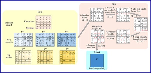
The workflow of FGS. The input to FGS includes the interaction matrix (|$\mathbf{Y}$|), drug similarities (|$\{\mathbf{S}^{d,h}\}_{h=1}^{3}$|) and LIC matrices (|$\{\mathbf{C}^{d,h}\}_{h=1}^{3}$|) computed according to Eq. (7). Diagonals of similarity matrices and LIC matrix values corresponding to non-interacting pairs (|$Y_{ij}=0$|), which are not used in FGS, are not shown in the figure for simplicity. We use |$k=2$| and |$\rho =1/3$| in this example, and similarity values of each drug’s 2-nearest neighbors (2NNs) are underlined. The whole procedure of FGS consists of six steps. (1) Initialize weight matrix using |$\mathbf{Y}$| and |$\{\mathbf{C}^{d,h}\}_{h=1}^{3}$|. (2) Complete zero-weights for known drugs (|$d_2$|). (3) Infer weights for new drugs (|$d_5$|), where |$W^d_{51}$| is the sum of |$W^d_{11}$| and |$W^d_{13}$| because |$d_1$| and |$d_3$| are the 2NNs of |$d_5$| in the first similarity view, and |$W^d_{52}$| (|$W^d_{53}$|) is the sum of |$d_3$| and |$d_4$|’s weight for |$\mathbf{S}^{d,2}$| (|$\mathbf{S}^{d,3}$|), i.e. |$W^d_{32}$| and |$W^d_{42}$| (|$W^d_{33}$| and |$W^d_{43}$|). (4) Select similarities by setting the smallest value in each row of the weight matrix to zero. (5) Normalize the weight matrix row-wise. (6) Integrate multiple similarities |$\{\mathbf{S}^{d,h}\}_{h=1}^{3}$| using fine-grained weight (|$\mathbf{W}^{d}$|) to obtain the fused similarity |$\mathbf{S}^{d}$|.
Initialization. In FGS, the local interaction consistency is employed to initialize the fine-grained weights due to its effectiveness in reflecting interaction distributions of proximate drugs. Specifically, given |$\{\mathbf{C}^{d,h}\}_{h=1}^{m_d}$| defined in Eq. (7), |$\mathbf{W}^{d}$| is initialized by aggregating all local interaction consistencies of interacting pairs for each drug similarity view:
Zero-Weights Completion for Known Drugs. There may be some known drugs whose similarity weights are all ‘0’s, i.e. |$\mathbf{W}^{d}_{i\cdot }=\mathbf{0}$|. The zero-weight vector indicates that all types of similarities regarding the corresponding drug are totally useless, which would lead to an invalid integration. To avoid this issue, we define a global weight vector |$\mathbf{v}^{d} = \sum _{i=1}^{n_d}\mathbf{W}^d_{i\cdot }$| which reflects the utility of each type of similarity over all drugs, and assign |$\mathbf{v}^d$| to all drugs associated with zero-valued weight vectors:
Inferring Weights for New Drugs. Since new drugs lack any known interacting target, their initialized weights, calculated according to Eq. (15), are all zeros as well. However, the global weight vector based imputation is not suitable for new drugs. As different new drugs may have different potential interactions, assigning a unique weight vector to every new drug fails to reveal their distinctive properties. In FGS, we extend the guilt-by-association principle, assuming that similarity weights of a drug are also approximate to its neighbors. Specifically, given a new drug |$d_x$|, we infer its weights by aggregating the weights of its |$k$| nearest known drugs in each similarity view:
Fine-Grained Similarity Selection. A lower local interaction consistency indicates that similar drugs usually interact with different targets, which further implies that noisy information is possessed by the corresponding similarity view. To mitigate the influence of noise, we conduct a fine-grained selective procedure to filter corrupted similarities for each drug by sparsifying the weight matrix. Specifically, for each row of |$\mathbf{W}^{d}$|, its |$\rho m_d$| smallest weights, whose corresponding similarities are considered as noisy, are set to 0:
where |$\mathcal{H}_i$| is a set containing indices of the |$\rho m_d$| smallest values in |$\mathbf{W}^{d}_{i\cdot }$|, and |$\rho$| is the filter ratio. Similarities with zero weights are discarded, while those with non-zero weights are eventually used to generate the integrated similarity matrix. Different from existing similarity selective strategies that delete whole similarity matrices, the selection process in FGS evaluates similarities at a finer granularity. For each similarity view, FGS gets rid of noisy similarities for some drugs, while retaining informative similarities for others. As shown in the step 4 of Figure 1, the first similarity view is filtered for drugs |$d_1$| and |$d_5$|, but retained for the rest three drugs.
Normalization. The row-wise normalization is applied to the fine-grained similarity weight matrix, so as to keep the range of similarity values unchanged:
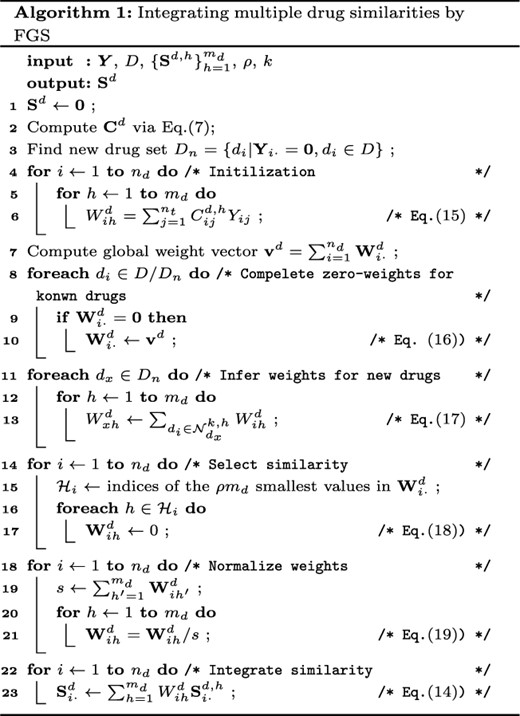
The process of fusing multiple drug similarities by FGS is summarized in Algorithm 1. The procedure of integrating target similarities with fine-grained weights is achieved in the same way, except for replacing |$Y_{ij}$| with |$Y_{ij}^\top$| in Eq. (15) and substituting superscript |$d$| with |$t$| in Eq. (14)-(19).
Computational Complexity Analysis
In FGS, the computational complexity of fine-grained weight initialization, including computing |$\{\mathbf{C}^{d,h}\}_{h=1}^{m_d}$|, is equal to |$O(m_d(n_d^2+n_dk\log (k)))$|. The computational costs of zero-weights imputation for known and new drugs are |$O(m_dn_d)$| and |$O(m_d|D_n|k\log (k))$|, respectively, where |$|D_n|$| is the number of new drugs. The computational complexity of similarity selection and weight normalization is |$O(m_dn_d)$|. Considering |$|D_n|<n_d$|, the computational complexity of the fine-grained weight calculation is |$O(m_d(n_d^2+n_dk\log (k)))$|. For weighted similarity integration, its computational complexity is |$O(m_dn_d^2)$|, which is the same as other conventional linear combination approaches using a singular weight value for each similarity matrix. The overall complexity of FGS is therefore |$O(m_d(n_d^2+n_dk\log (k)))$|.
Overview of Similarity Integration Methods
Table 1 summarizes the characteristics and computational complexity of the proposed FGS and other similarity integration methods introduced in Section 3.2.
Summarization of Similarity Integration Approaches.
| Method | Type | Supervised | Capturing entity-wise utility | Computational complexity | ||
|---|---|---|---|---|---|---|
| Similarity selection | Similarity integration | Weight calculation | Similarity integration | |||
| AVE [2] | Linear | |$\times$| | - | |$\times$| | |$O(m_d)$|. | |$O(m_dn_d^2)$| |
| KA [19] | Linear | |$\checkmark$| | - | |$\times$| | |$O(m_dn_d^2)$| | |$O(m_dn_d^2)$| |
| HSIC [17] | Linear | |$\checkmark$| | - | |$\times$| | |$O(m_dn_d^3+rm_d^3)$| | |$O(m_dn_d^2)$| |
| LIC [16] | Linear | |$\checkmark$| | - | |$\times$| | |$O(m_d(n_d^2+n_d k\log (k)+|P_1|))$| | |$O(m_dn_d^2)$| |
| SNF-H [15] | nonlinear | |$\times$| | |$\times$| | |$\checkmark$| | - | |$O(rm^{\prime}_dn_d^3)$| |
| SNF-F [21] | nonlinear | |$\checkmark$| | |$\times$| | |$\checkmark$| | - | |$O(m_d^2\Theta (n_d,n_t)+rm^{\prime}_dn_d^3)$| |
| FGS (ours) | Linear | |$\checkmark$| | |$\checkmark$| | |$\checkmark$| | |$O(m_d(n_d^2+n_dk\log (k)))$| | |$O(m_dn_d^2)$| |
First, compared with other linear similarity integration approaches, FGS incorporates similarity selection to filter noisy information and is aware of the distinctive properties of drugs (targets) in each similarity view. In addition, the computational complexity of similarity integration in FGS is the same as other linear methods, which is linear to the number of similarity views and quadratic to the number of drugs (targets).
The advantages of FGS over nonlinear methods are twofold. First, FGS selects similarity at a fine granular perspective, while the two nonlinear methods discard whole similarities without considering the entity-wise utility of similarity views. Second, FGS is more computationally efficient than the two SNF-based approaches, whose computational cost is cubic to the number of drugs (targets).
EXPERIMENTS
Dataset
In the experiments, we utilize five benchmark DTI datasets, including four collected by Yamanishi [26], namely Nuclear Receptors (NR), G-protein coupled receptors (GPCR), Ion Channel (IC) and Enzyme (E), and one obtained from [22] (denoted as Luo). Table 2 summarizes the information of these datasets. More details on similarity calculations can be found in Supplementary Section A2.
Characteristic of DTI datasets, where different colors denotes similarities derived from data diverse sources.
| Dataset | NR | GPCR | IC | E | Luo |
|---|---|---|---|---|---|
| Drug | 54 | 223 | 210 | 445 | 708 |
| Target | 26 | 95 | 204 | 664 | 1512 |
| Interaction | 166 | 1096 | 2331 | 4256 | 1923 |
| Sparsity | 0.118 | 0.052 | 0.054 | 0.014 | 0.002 |
| Drug Similarity (Source) |$^\ddag$| | SIMCOMP, LAMBDA, MARG, MINMAX, SPEC, TAN (CS) ; AERS-b, AERS-f, SIDER (SE) | TAN (CS), DDI, DIA, SE | |||
| Target Similarity (Source)|$^\S$| | SW, MIS-k3m1, MIS-k4m1, MIS-k3m2, MIS-k4m2, SPEC-k3, SPEC-k4 (AAS) ; PPI; GO | SW (AAS), PPI, TIA | |||
|$\ddag$| CS: chemical structure, SE: drug side effect, DDI: drug–drug interaction, DIA: drug–disease association |$\S$| AAS: amino-acid sequence, PPI: protein–protein interaction, GO: Gene Ontology annotation, TIA: target–disease association
Yamanishi datasets only contain interactions discovered before they were constructed (in 2007). Therefore, we update them by adding newly discovered DTIs recorded in the up-to-date version of KEGG, DrugBank and ChEMBL databases [27]. There are 175, 1350, 3201 and 4640 interactions in the updated NR, GPCR, IC and E datasets. Nine drug and nine target similarities from [2] are used to describe the drug and target relations in various aspects. Six drug similarities are constructed based on chemical structure (CS) with various metrics, while the other three are derived from drug side effects (SE). Seven target similarities are calculated based on protein amino-acid sequence (AAS) using different similarity assessments, while the other two are obtained from Gene Ontology (GO) terms and protein–protein interactions (PPI), respectively.
Luo dataset includes 1923 DTIs obtained from DrugBank 3.0. The similarities of the Luo dataset are obtained from [22]. Specifically, four types of drug similarity are computed based on CS, drug–drug interactions (DDI), SE and drug–disease associations (DIA). Three kinds of target similarities are derived from AAS, PPI and target–disease associations (TIA).
Experiment Setup
In the empirical study, we first compare the proposed FGS with six similarity integration methods, namely AVE [2], KA [19], HSIC [17], LIC [16], SNF-H [15] and SNF-F [21]. The similarity integration method needs to collaborate with a DTI prediction model to infer unseen interactions. Therefore, we employ five DTI prediction approaches, including WKNNIR [9], NRLMF [8], GRMF [7], BRDTI [28] and DLapRLS [17], as base models of similarity integration methods. Each base model is trained on the fused drug and target similarities generated by each similarity integration method. Within each base model, better prediction performance indicates the superiority of the corresponding similarity integration approach.
In addition, we further compare FGS, which collaborates with well-performing base models, with state-of-the-art DTI prediction models that can directly handle heterogeneous information. Specifically, the competitors include four traditional machine learning-based approaches (MSCMF [18], KRLSMKL [2], MKTCMF [3] and NEDTP [4]) and four deep learning models (NeoDTI [23], DTIP [5], DCFME [24] and SupDTI [25]).
To verify the effectiveness of our method, three more challenging prediction settings that estimate interactions for new drugs and/or new targets are considered. Three types of cross validation (CV) are utilized accordingly [29]:
CVS|$_d$|: 10-fold CV on drugs to predict DTIs between new drugs and known targets, where one drug fold is split as a test set.
CVS|$_t$|: 10-fold CV on targets to predict DTIs between known drugs and new targets, where one target fold is split as a test set.
CVS|$_{dt}$|: |$3 \times 3$|-fold CV on both drugs and targets to infer DTIs between new drugs and new targets, where one drug fold and one target fold are split as a test set.
Area under the precision-recall curve (AUPR) and the receiver operating characteristic curve (AUC) are employed as evaluation metrics. In FGS, we set |$k=5$| for all datasets. The filter ratio |$\rho$| is set as 0.5 for Yamanishi datasets. For the Luo dataset, |$\rho =0.2$| in CVS|$_d$| and CVS|$_{dt}$| and |$\rho =0.7$| in CVS|$_t$|. The hyperparameters of comparing similarity integration methods, DTI prediction models and base prediction models are set based on the suggestions in the respective articles or chosen by grid search (see Supplementary Table A1 and Section A3).
FGS versus Similarity Integration Methods
Table 3 summarizes the average ranks of FGS and the six similarity integration competitors with the five base prediction models. Detailed results can be found in Supplementary Tables A2–A7. FGS achieves the best average rank under all prediction settings in terms of both AUPR and AUC. Furthermore, as shown in Table 4, FGS achieves statistically significant improvement over all competitors under all three prediction settings, according to the Wilcoxon signed-rank test with Bergman–Hommel’s correction [30] at 5% level. This demonstrates the effectiveness of the selective fine-grained weighting scheme in FGS. LIC and SNF-F are the second and third methods. Although LIC also relies on local interaction consistency-based weights, it does not include fine-grained similarity weighting and selection. SNF-F is outperformed by FGS, mainly because its global similarity selection cannot exploit the utility of similarity views for individual drugs and targets. The following two methods, KA and HSIC, do not remove noisy information and do not exploit the entity-wise similarity utility. AVE and SNF-F are the two worst approaches, since they totally ignore any interaction information, which is vital in the DTI prediction task.
Average ranks of similarity integration methods under three prediction settings.
| Metric | Setting | AVE | KA | HSIC | LIC | SNF-H | SNF-F | FGS |
|---|---|---|---|---|---|---|---|---|
| AUPR | CVS|$_d$| | 5.3 | 4.7 | 4.4 | 2.52 | 6.68 | 3.2 | 1.2 |
| CVS|$_t$| | 5.26 | 4.14 | 4.8 | 2.9 | 5.04 | 3.92 | 1.94 | |
| CVS|$_{dt}$| | 5.3 | 4.9 | 4.8 | 2.44 | 6.92 | 2.24 | 1.4 | |
| Summary | 5.29 | 4.58 | 4.67 | 2.62 | 6.21 | 3.12 | 1.51 | |
| AUC | CVS|$_d$| | 4.98 | 4.65 | 4.48 | 2.73 | 6.85 | 2.78 | 1.55 |
| CVS|$_t$| | 4.43 | 4.45 | 4.08 | 3.3 | 5.73 | 3.48 | 2.55 | |
| CVS|$_{dt}$| | 5.38 | 4.83 | 4.8 | 2.8 | 6.25 | 2.5 | 1.45 | |
| Summary | 4.93 | 4.64 | 4.45 | 2.94 | 6.28 | 2.92 | 1.85 |
P-values of Wilcoxon signed-rank test with Bergman–Hommel’s correction at 5% level for similarity integration methods under each prediction setting, where P-values less than 0.05 are highlighted by bold to indicate that FGS achieves statistically significant improvement over the corresponding competitor.
| Metric | Setting | AVE | KA | HSIC | LIC | SNF-H | SNF-F |
|---|---|---|---|---|---|---|---|
| AUPR | CVS|$_d$| | 1.3e-4 | 1.3e-4 | 1.3e-4 | 1.3e-4 | 1.3e-4 | 1.3e-4 |
| CVS|$_t$| | 2.4e-4 | 5.0e-4 | 2.4e-4 | 6.9e-4 | 4.8e-3 | 4.8e-2 | |
| CVS|$_{dt}$| | 1.3e-4 | 1.3e-4 | 1.3e-4 | 2.6e-4 | 1.3e-4 | 7.7e-3 | |
| AUC | CVS|$_d$| | 1.3e-4 | 1.3e-4 | 1.3e-4 | 5.2e-4 | 1.3e-4 | 5.3e-4 |
| CVS|$_t$| | 5.9e-3 | 4.7e-3 | 5.9e-3 | 9.7e-3 | 3.8e-4 | 3.9e-2 | |
| CVS|$_{dt}$| | 1.3e-4 | 1.3e-4 | 1.3e-4 | 1.4e-4 | 1.3e-4 | 2.6e-2 |
Figure 2 shows the runtime of FGS and other baselines for integrating drug and target similarities of the E dataset. AVE and KA are the two fastest methods due to their efficient linear fusion strategy. LIC and the proposed FGS are slower than the top two, because they search kNNs to calculate the local interaction consistency. The nonlinear approach, SNF-H, which has a cubic computational complexity w.r.t. the drug (target) size, is the fifth. HSIC requires solving a quadratic optimization problem, which leads to the most time-consuming integration procedure.
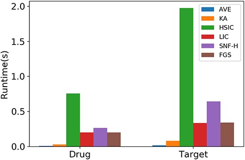
Runtime of similarity integration methods on E dataset.
We further examine the robustness of FGS w.r.t. the variation of base model hyperparameters as well as the test set without homologous drugs, and analyze the sensitivity of hyperparameters in FGS. See Supplementary Section A4.2, A4.3 and A4.4 for more details.
AUPR Results of FGS with WkNNRI and traditional machine learning based competitors.
| Setting | Dataset | MSCMF | KRLSMKL | MKTCMF | NEDTP | FGSWkNNRI |
|---|---|---|---|---|---|---|
| CVS|$_d$| | NR | 0.44(4) | 0.474(3) | 0.415(5) | 0.486(2) | 0.551(1) |
| GPCR | 0.46(2) | 0.302(5) | 0.417(4) | 0.451(3) | 0.547(1) | |
| IC | 0.408(2) | 0.236(5) | 0.337(4) | 0.407(3) | 0.486(1) | |
| E | 0.231(4) | 0.208(5) | 0.256(3) | 0.33(2) | 0.418(1) | |
| Luo | 0.371(4) | 0.452(3) | 0.485(2) | 0.077(5) | 0.49(1) | |
| AveRank | 3.2 | 4.2 | 3.6 | 3 | 1 | |
| CVS|$_t$| | NR | 0.466(4) | 0.497(2) | 0.49(3) | 0.375(5) | 0.565(1) |
| GPCR | 0.583(4) | 0.579(5) | 0.726(2) | 0.684(3) | 0.776(1) | |
| IC | 0.781(4) | 0.744(5) | 0.849(2) | 0.8(3) | 0.855(1) | |
| E | 0.574(4) | 0.464(5) | 0.708(2) | 0.615(3) | 0.725(1) | |
| Luo | 0.08(4) | 0.21(3) | 0.248(2) | 0.046(5) | 0.459(1) | |
| AveRank | 4 | 4 | 2.2 | 3.8 | 1 | |
| CVS|$_{dt}$| | NR | 0.228(3) | 0.191(4) | 0.242(2) | 0.16(5) | 0.251(1) |
| GPCR | 0.284(3) | 0.239(5) | 0.248(4) | 0.29(2) | 0.389(1) | |
| IC | 0.232(3) | 0.131(5) | 0.199(4) | 0.251(2) | 0.339(1) | |
| E | 0.1(3) | 0.091(4) | 0.084(5) | 0.112(2) | 0.241(1) | |
| Luo | 0.018(5) | 0.125(3) | 0.129(2) | 0.03(4) | 0.203(1) | |
| AveRank | 3.4 | 4.2 | 3.4 | 3 | 1 | |
| Summary | 3.53 | 4.13 | 3.07 | 3.27 | 1 | |
| p-value | 3.2e-3 | 3.2e-3 | 3.2e-3 | 3.2e-3 | - | |
AUC Results of FGS with WkNNRI and traditional machine learning based competitors.
| Setting | Dataset | MSCMF | KRLSMKL | MKTCMF | NEDTP | FGSWkNNRI |
|---|---|---|---|---|---|---|
| CVS|$_d$| | NR | 0.779(5) | 0.787(2) | 0.785(4) | 0.786(3) | 0.825(1) |
| GPCR | 0.884(3) | 0.839(5) | 0.855(4) | 0.885(2) | 0.911(1) | |
| IC | 0.795(2) | 0.767(4) | 0.764(5) | 0.794(3) | 0.863(1) | |
| E | 0.75(5) | 0.819(3) | 0.763(4) | 0.837(2) | 0.875(1) | |
| Luo | 0.897(3) | 0.855(5) | 0.89(4) | 0.907(1) | 0.905(2) | |
| AveRank | 3.6 | 3.8 | 4.2 | 2.2 | 1.2 | |
| CVS|$_t$| | NR | 0.755(4) | 0.759(3) | 0.776(2) | 0.726(5) | 0.817(1) |
| GPCR | 0.891(4) | 0.889(5) | 0.916(3) | 0.918(2) | 0.95(1) | |
| IC | 0.941(3) | 0.935(5) | 0.948(2) | 0.939(4) | 0.958(1) | |
| E | 0.902(3.5) | 0.897(5) | 0.902(3.5) | 0.918(2) | 0.933(1) | |
| Luo | 0.826(5) | 0.9(1) | 0.841(4) | 0.86(3) | 0.862(2) | |
| AveRank | 3.9 | 3.8 | 2.9 | 3.2 | 1.2 | |
| CVS|$_{dt}$| | NR | 0.581(3) | 0.552(4) | 0.616(1) | 0.548(5) | 0.603(2) |
| GPCR | 0.814(3) | 0.792(4) | 0.729(5) | 0.816(2) | 0.869(1) | |
| IC | 0.701(3) | 0.637(5) | 0.65(4) | 0.702(2) | 0.768(1) | |
| E | 0.742(4) | 0.754(2) | 0.619(5) | 0.744(3) | 0.821(1) | |
| Luo | 0.752(4) | 0.795(3) | 0.671(5) | 0.822(2) | 0.862(1) | |
| AveRank | 3.4 | 3.6 | 4 | 2.8 | 1.2 | |
| Summary | 3.63 | 3.73 | 3.7 | 2.73 | 1.2 | |
| p-value | 3.2e-3 | 3.2e-3 | 3.2e-3 | 3.2e-3 | - | |
FGS with Base Models versus DTI Prediction Models
In this part, we first compare the proposed FGS combined with WkNNRI, denoted as FGSWkNNRI, with four traditional machine learning-based DTI prediction methods, namely MSCMF, KRLSMKL, MKTCMF and NEDTP, that can directly handle multiple types of similarities. The AUPR and AUC results in three prediction settings are shown in Tables 5 and 6, respectively. FGSWkNNRI is the best method and significantly outperforms all competitors, according to the Wilcoxon signed-rank statistical test with Bergman–Hommel on the results of all prediction settings. This demonstrates the effectiveness of the proposed fine-grained selective similarity fusion manner to extract vital information from multiple similarities. There are some cases, e.g. the Luo dataset in CVS|$_d$| and CVS|$_t$| and the NR dataset in CVS|$_{dt}$|, where AUC results of FGS are slightly lower than the corresponding best comparison method (NEDTP, KronRLSMKL and MKTCMF). Nevertheless, in these cases, the three competitors perform much worse than FGS in AUPR, which is more informative in assessing a model under the extremely sparse interaction distribution.
Furthermore, FGS is compared with four deep learning based DTI prediction models, including NeoDTI, DTIP, DCFME and SupDTI. These four deep learning competitors, inferring new DTIs by mining heterogeneous networks, can only handle the Luo dataset, which could be formulated as a heterogeneous DTI network containing four types of nodes (drugs, targets, diseases and side effects). Besides, considering that the four deep learning competitors mainly focus on predicting new DTIs between known drugs and known targets, we utilize the 10-fold CVs on drug–target pairs, named CVS|$_p$|, to simulate this prediction setting. GRMF and NRLMF that can be applied to CVS|$_p$| are used as the base model of FGS. As per the results shown in Table 7, FGSGRMF and FGSNRLMF are the top two methods in terms of AUPR, which achieve 6.7% and 2.5% improvement over the best baseline (DCFME). DTIP attains the best AUC result, followed by FGSGRMF and FGSNRLMF that are 4.4% and 2.8% lower. However, DTIP suffers a huge decline in AUPR, indicating that it heavily emphasizes the AUC results at the expense of a decrease in AUPR.
Overall, the comparison with various state-of-the-art DTI prediction models under different prediction settings confirms the superiority of FGS.
Investigation of Similarity Weights
Similarity weights play a vital role in the linear similarity integration method, determining the contribution of each view to the final fused similarity space. Hence, we further investigate drug similarity weights on the GPCR dataset generated by FGS and four linear methods.
Results of FGS with GRMF and NRLMF and deep learning competitors on Luo dataset under CVS|$_p$|.
| Metric | NeoDTI | DTIP | DCFME | SupDTI | FGSGRMF | FGSNRLMF |
|---|---|---|---|---|---|---|
| AUPR | 0.573(5) | 0.399(6) | 0.596(3) | 0.585(4) | 0.639(1) | 0.611(2) |
| AUC | 0.921(6) | 0.981(1) | 0.936(4) | 0.933(5) | 0.939(3) | 0.954(2) |
| Metric | NeoDTI | DTIP | DCFME | SupDTI | FGSGRMF | FGSNRLMF |
|---|---|---|---|---|---|---|
| AUPR | 0.573(5) | 0.399(6) | 0.596(3) | 0.585(4) | 0.639(1) | 0.611(2) |
| AUC | 0.921(6) | 0.981(1) | 0.936(4) | 0.933(5) | 0.939(3) | 0.954(2) |
As shown in Figure 3, AVE assigns equal weight to each type of similarity. KA increases the importance of CS-based similarities. HSIC considers SIMCOMP, LAMBDA, MARG and AERS-b similarities more informative than others. LIC emphasizes SIMCOMP and three SE-based similarities. All the above four methods do not discard any noisy similarity, i.e. all weights are nonzero. FGS produces different weight vectors for each drug, so two representative drugs in the GPCR dataset, namely D00559 (pramipexole) and D00607 (guanadrel), are considered in this case study.
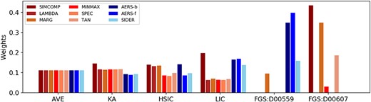
Drug similarity weights for the GPCR dataset. The various red and blue bars denote the weights of different chemical structure (CS) and side effect (SE)-based similarities, respectively.
Pramipexole, a commonly used Parkinson’s disease (PD) medication, interacts with three types of dopaminergic receptors, e.g. DRD2, DRD3 and DRD4, whose genetic polymorphisms are potential determinants of PD development, symptoms and treatment response [31]. D00059 (levodopa), which also interacts with dopaminergic receptors, could be combined with pramipexole to relief the symptoms in PD [32, 33]. The two drugs frequently coexist in reported adverse events, resulting in larger AERS-f and AERS-b similarities. Nevertheless, their chemical structures are discrepant, since they do not share many common substructures. Pramipexole (Figure 4 (A)) is a member of the class of benzothiazoles (C7H5NS) in which the hydrogens at the 2 and 6-pro-S-positions are substituted by amino (-NH2) and propylamino groups (C3H9N), respectively. While levodopa (Figure 4 (B)) is a hydroxyphenylalanine (C9H11NO3) carrying hydroxy substituents (-OH) at positions 3 and 4 of the benzene ring. Therefore, for pramipexole, FGS assigns higher weights to SE-based similarities that are more reliable in identifying drugs interacting with the same targets as pramipexole (e.g. levodopa), and treats most CS-based ones as noise.
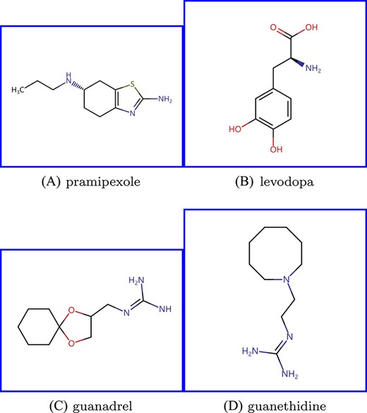
Chemical structures of (A) pramipexole, (B) levodopa, (C) guanadrel and (D) guanethidine.
Guanadrel is an antihypertensive that inhibits the release of norepinephrine from the sympathetic nervous system to suppress the responses mediated by alpha-adrenergic receptors, leading to the relaxation of blood vessels and the improvement of blood circulation [34, 35]. D02237 (guanethidine), another medication to treat hypertension, is pharmacologically and structurally similar to guanadrel, which also interacts with alpha-adrenergic receptors and is identified as the most similar drug to guanadrel based on the SIMCOMP similarity. As shown in Figure 4 (C) and (D), both of them include guanidine (CH5N3). On the other hand, the side effects of guanadrel and guanethidine are not included in the SIDER database and are merely recorded in AERS, causing the invalidity of SE-based similarities. Therefore, when it comes to guanadrel, FGS emphasizes CS-based similarities and discards all SE-based ones.
Compared with other linear integration methods, FGS not only distinguishes the importance of similarities for each drug based on the corresponding pharmacological properties, but also diminishes the influence of noisy similarities.
Discovery of New DTIs
We check the validity of novel DTIs discovered by FGS from the Luo dataset. Specifically, we leverage 10-fold CVs on non-interacting pairs, i.e. using all interacting pairs and nine folds of non-interacting pairs as the training set, and leaving the remaining non-interacting fold as the test set. The top 10 non-interacting pairs with the highest prediction scores across all 10 folds are considered new interacting candidates. Table 8 lists the new DTIs found by FGSGRMF and FGSNRLMF, along with their supportive evidence retrieved from DrugBank (DB) [36] and DrugCentral (DC) [37] databases. There are 18 out of 20 new interactions confirmed by at least one database, which is comparable with other similarity integration methods (Supplementary Table A10), demonstrating the effectiveness of FGS in trustworthy new DTI discovery. In addition, compared with new DTIs predicted by other similarity integration methods (Supplementary Tables A8–A9), there are three novel DTIs (bold ones in Table 8) only discovered by FGS, including two unverified ones.
Top 10 new DTIs discovered by FGSGRMF and FGSNRLMF from the Luo dataset.
| Rank | FGS|$_{\textrm GRMF}$| | FGS|$_{\textrm NRLMF}$| | ||||||||
|---|---|---|---|---|---|---|---|---|---|---|
| Drug ID | Drug Name | Target ID | Target Name | Database | Drug ID | Drug Name | Target ID | Target Name | Database | |
| 1 | DB00829 | Diazepam | P48169 | GABRA4 | DB | DB00829 | Diazepam | P48169 | GABRA4 | DB |
| 2 | DB01215 | Estazolam | P48169 | GABRA4 | DB | DB01215 | Estazolam | P48169 | GABRA4 | DB |
| 3 | DB00363 | Clozapine | P21918 | DRD5 | DC | DB00363 | Clozapine | P21918 | DRD5 | DC |
| 4 | DB00734 | Risperidone | P28222 | HTR1B | DC | DB06216 | Asenapine | P21918 | DRD5 | DC |
| 5 | DB06800 | Methylnaltrexone | P41143 | OPRD1 | DC | DB06216 | Asenapine | P28221 | HTR1D | DC |
| 6 | DB00652 | Pentazocine | P41143 | OPRD1 | DC | DB00696 | Ergotamine | P08908 | HTR1A | DB, DC |
| 7 | DB06216 | Asenapine | P21918 | DRD5 | DC | DB00543 | Amoxapine | P28223 | HTR2A | DB, DC |
| 8 | DB00333 | Methadone | P41145 | OPRK1 | DC | DB00652 | Pentazocine | P41143 | OPRD1 | DC |
| 9 | DB06216 | Asenapine | P28221 | HTR1D | DC | DB01273 | Varenicline | Q15822 | CHRNA2 | - |
| 10 | DB00734 | Risperidone | P21918 | DRD5 | DC | DB01186 | Pergolide | P34969 | HTR7 | - |
For the two drug–target pairs (DB01273-Q15822 and DB01186-P34969) that have not been recorded in the databases, we check their binding affinities by conducting docking simulations with PyRx1 . The 2D and 3D visualizations of docking interactions of DB01273 with Q15822 and DB01186 with P34969, produced by Discovery Studio2 , are shown in Figure 5 and Supplementary Figure A6. The binding energy between DB01273 and Q15822 is -8.9 kcal|$\backslash \textrm{mol}$|. DB01273 binds with Q15822 by forming a Pi-alkyl bond with Lys104, an attractive charge and a carbon hydrogen bond with Glu80 and Van der Waals bonds with nine amino acid residues. DB01273 (varenicline) is a medicine for smoking cessation via partial agonists at nicotinic acetylcholine receptors, which is more likely to interact with Q15822 (CHRNA2, alpha-2 subtype of neuronal acetylcholine receptor). Regarding DB01186 and P34969, 13 residues of P34969 are involved in Van der Waals interactions, five residues are bonded to DB01186 through Pi-alkyl or alkyl interactions and Met193 is also linked with the ligand through carbon–hydrogen interaction, which results in the binding score of -7.2 kcal|$\backslash \textrm{mol}$|. DB01186 (pergolide), a treatment for Parkinson’s Disease, interacts with 5-hydroxytryptamine receptors (HTR1A, HTR2B, HTR1D, etc.) that have similar function (serotonin receptor activity) with P34969 (HTR7). The docking results of two drug–target pairs indicate that their potential interactions are reliable.
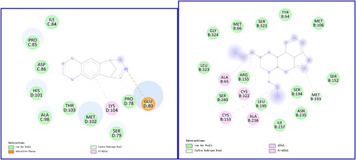
2D visualization of docking results. The left figure shows docking interactions of DB01273 (varenicline) with Q15822 (CHRNA2), and the right figure presents docking interactions of DB01186 (pergolide) with P34969 (HTR7)
CONCLUSION
This paper proposed FGS, a fine-grained selective similarity integration approach, to produce more compact and beneficial inputs for DTI prediction models via entity-wise utility-aware similarity selection and fusion. We conducted extensive experiments under various DTI prediction settings, and the results demonstrate the superiority of FGS to the state-of-the-art similarity integration methods and DTI prediction models with the cooperation of simple base models. Furthermore, the case studies verify the importance of the fine-grained similarity weighting scheme and the practical ability of FGS to assist prediction models in discovering reliable new DTIs.
In the future, we plan to extend our work to handle heterogeneous information from multi-modal views, i.e. drug and target information in different formats, such as drug chemical structure graphs, target genomic sequences, textual descriptions from scientific literature and vectorized feature representations.
FGS is an entity-wise utility-aware similarity integration approach that generates a reliable fused similarity matrix for any DTI prediction model by capturing crucial information and removing noisy similarities at a finer granularity.
Extensive experimental studies on five public DTI datasets demonstrate the effectiveness of FGS.
Case studies further exemplify that the fine-grained similarity weighting scheme used in FGS is more suitable than conventional ones for DTI prediction with multiple similarities.
FUNDING
This work was partially supported by Science Innovation Program of Chendu-Chongqing Economic Circle in Southwest China (grant no. KJCXZD2020027)
DATA AND CODE AVAILABILITY
The source code and data of this work can be found at https://github.com/Nanfeizhilu/FGS_DTI_Predition
Footnotes
Bin Liu is a lecturer at Key Laboratory of Data Engineering and Visual Computing, Chongqing University of Posts and Telecommunications. His research interests include multi-label learning and bioinformatics.
Jin Wang is a Professor at Key Laboratory of Data Engineering and Visual Computing, Chongqing University of Posts and Telecommunications. His research interests include large scale data mining and machine learning.
Kaiwei Sun is an Associate Professor at Key Laboratory of Data Engineering and Visual Computing, Chongqing University of Posts and Telecommunications. His research interests in data mining and machine learning.
Grigorios Tsoumakas is an Associate Professor at the Aristotle University of Thessaloniki. His research interests include machine learning (ensembles, multi-target prediction) and natural language processing (semantic indexing, keyphrase extraction, summarization)
References
