


Abstract
A large number of works have presented the single-cell RNA sequencing (scRNA-seq) to study the diversity and biological functions of cells at the single-cell level. Clustering identifies unknown cell types, which is essential for downstream analysis of scRNA-seq samples. However, the high dimensionality, high noise and pervasive dropout rate of scRNA-seq samples have a significant challenge to the cluster analysis of scRNA-seq samples. Herein, we propose a new adaptive fuzzy clustering model based on the denoising autoencoder and self-attention mechanism called the scDASFK. It implements the comparative learning to integrate cell similar information into the clustering method and uses a deep denoising network module to denoise the data. scDASFK consists of a self-attention mechanism for further denoising where an adaptive clustering optimization function for iterative clustering is implemented. In order to make the denoised latent features better reflect the cell structure, we introduce a new adaptive feedback mechanism to supervise the denoising process through the clustering results. Experiments on 16 real scRNA-seq datasets show that scDASFK performs well in terms of clustering accuracy, scalability and stability. Overall, scDASFK is an effective clustering model with great potential for scRNA-seq samples analysis. Our scDASFK model codes are freely available at https://github.com/LRX2022/scDASFK.
Introduction
Many biological problems involve DNA sequence analysis. Each cell has its unique type and biological function, reflected in the differences between different histology [1]. In recent years, single-cell RNA sequencing (scRNA-seq) has developed rapidly’ and it is a technique that targets the genome or transcriptome of a single cell for sequencing analysis at the single-cell level. scRNA-seq enables more precise measurements of gene expression levels and detects minute amounts of gene expression or rare non-coding RNA. It is essential to discriminate undetected cell types and predict cell states in complex diseases, inferring cell pseudo time trajectories and revealing both gene architecture and cell heterogeneity [2, 3].
Efficient identification of cell types primarily affects the downstream analysis of scRNA-seq samples. However, the low capture efficiency and high missed detection rate of the current scRNA-seq technology, scRNA-seq data are often characterized by high dimensionality, high noise and sparse, which brings great difficulties in identifying and analyzing single-cell samples. Therefore, an efficient method to cluster group scRNA-seq data is urgently needed. In the past few years, a large number of clustering methods for scRNA-seq data have been proposed and developed. For example, GiniClust [4] employs the Gini index to select genes to reduce the dimensionality of the data, and the effect of reducing data noise before cell classification is achieved through density-based clustering. RaceID [5] captures the relationships between cells according to the Pearson correlation coefficient and serves as an input for K-means clustering [6] to identify cell types. SNN-Cliq [7] introduces relationships between cells by constructing a shared nearest neighbor (SNN) and employs quasi-clique-based clustering models to search for potential cell types. Seurat [8, 9] combines in situ RNA data to spatially locate cells, and SNN maps are constructed in later updates and employ the Louvain algorithm to cluster assignments [10]. This community detection algorithm assigns nodes to the community greedily and is more scalable than other graph-based algorithms. CellTree [11] generates the theme histogram based on a document analysis technique—LDA [12] and builds a minimum spanning tree based on a chi-square to find relationships between cells.
However, the characteristics of high noise and sparsity of scRNA-seq data seriously affect the validity and reliability of similarity metric methods and graph structure-based clustering algorithms in classifying single-cell data. SIMLR [13] solves the effect of high noise on clustering accuracy by multi-kernel learning to obtain better cell similarity. SC3 [14] employs Euclidean, Pearson and Spearman to learn cell similarity from different perspectives and employs consensus clustering to get the final result. SCENA [15] obtains multiple cell similarity matrices from different dimensions of single cell data and employs a local affinity matrix to update the similarity matrix to enhance the relationships between cells, then employs consensus clustering to obtain the results. Although these ensemble learning-based methods attenuate the effect of data noise on clustering results, it is difficult to mine the latent information of data, and the growing amount of data with the development of scRNA-seq makes the computational cost of such algorithms substantially increase. SHARP [16] processes large datasets in parallel through a divide-and-conquer strategy and Random projection [17] to reduce computational costs and employs voting strategies to integrate multiple cluster results in its clustering process. However, it is still unable to obtain the latent features of the data for clustering. Overall, traditional machine learning methods are not friendly to large scRNA-seq datasets, and it is difficult to extract latent information in scRNA-seq datasets.
In recent years, deep learning [18] has received great attention as an essential part of machine learning and has been widely used in various scRNA-seq analysis tasks. Deep learning has a powerful fitting ability to approximate any complex function that learns latent information from complex datasets. It does not rely on prior knowledge and can automatically extract essential features from data through end-to-end learning. In addition, deep learning methods handle multiple tasks through a single model or can be adjusted to perform different tasks, which is highly scalable, and the effect of the deep model is more significant with the increase of data [19]. These advantages make deep learning perfectly matched to the characteristics of scRNA-seq data and more attractive to the growing single-cell data.
With the development of deep learning technology, many deep network-based models have been developed. For example, deep count autoencoder network (DCA) [20] proposes a zero inflation negative binomial (ZINB) [21] autoencoder for data denoising better to learn latent features from scRNA-seq data for subsequent clustering. scDeepCluster [22] is a deep embedded clustering method based on the DCA framework developed. It maps scRNA-seq data to a low-dimensional potential space by the ZINB model-based autoencoder while the clustering is performed based on Kullback–Leibler divergence between two distributions. scGMAI [23] is a Gaussian mixture model based on an autoencoder. It reconstructs the log-transformed expression matrix with dropout through an autoencoder. After imputation of the data, it employs fast and independent component analysis (FastICA) [24] for dimensionality reduction and finally employs a Gaussian mixture model to achieve the clustering. Although DCA, scDeepCluster and scGMAI can extract potential features from data, they ignore the relationships between cells, which may make the learned features inaccurate. GraphSCC [25] studies the structural relationship between cells through graph convolution network [26] and combines denoising autoencoder (DAE) [27] to optimize two networks simultaneously through a dual self-supervised module to achieve clustering. scGAE [28] employs multitask graph autoencoder to map high-dimensional data to low-dimensional space while capturing the structural and feature information of the data to achieve a better clustering effect. However, the deep networks used in these models require pretraining and cannot adaptively extract latent cell information for clustering.
To overcome these problems, we propose a deep clustering model (scDASFK) based on DAE and self-attention [29] for efficiently cluster assignments of scRNA-seq data. Specifically, we employ DAE and the idea of the deep adaptive clustering model [30] to denoise the data to enhance the overall robustness of the model, while capturing the relationship between cells and reducing the data dimension. Next, self-attention is used to extract critical features from the low-dimensional latent features again for clustering. However, such preliminary denoising may lose much valuable information, making it challenging to sufficiently represent the original data structure. Therefore, we propose an adaptive feedback mechanism to enable the designed model further to retain as much valuable information as possible and reduce the impact of noise on the final results.
To evaluate the performance of scDASFK, we compare it with six advanced machine learning methods and three deep clustering methods to illustrate the advantages of scDASFK in analyzing scRNA-seq data. We also prove that scDASFK has a good denoising ability through visualization and dimensionality reduction experiments.
Materials and methods
Datasets
In the experiments, we consider for comparison with the highly competitive scRNA-seq datasets, then present thorough experiments demonstrating the efficacy and value of the proposed technique. We evaluate our method on a total of 16 scRNA-seq datasets containing different human and mouse tissues, of which 12 are public datasets that can be downloaded from the website (https://hemberg-lab.github.io/scRNA.seq.datasets/), Lawlor [31] and Muraro [32] are two datasets containing unknown cell types, Bmcite [33] and Bhattacherjee [34] are two datasets with more than 10 000 cells. The details of these datasets is shown in Supplementary Table S1.
Preprocessing
We use the Python package SCANPY [35] to preprocess the original scRNA-seq data. scRNA-seq data are a matrix whose rows represent cells and columns represent genes, and each cell has the same number of genes. For such data, we remove genes with zero counts in more than 95% of cells in each dataset to reduce the impact of useless genes on model calculation and clustering accuracy, and normalize the data to the range with mean value of 0 and variance of 1, and then log transform the data. We select the top 3000 highly variable genes as the input data for scDASFK.
Model structure of scDASFK
The overall structure of scDASFK is shown in Figure 1. The scDASFK model is composed of two parts: deep denoising network (DN) and deep clustering network (CN). In order to better remove the effect of noise in the data on the model, we propose an adaptive feedback mechanism that introduces clustering information into the deep DN to optimize the two networks jointly. In this way, the denoised data can more accurately reflect the real data situation and get better clustering results.
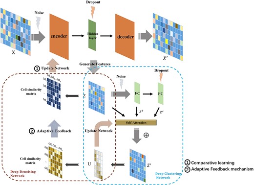
The overall structure of scDASFK. scDASFK consists of two models,i.e., deep DN and deep CN. It takes the pretreated gene expression matrix |$X$| as the input. The deep DN extracts the latent feature |$Z$| of |$X$|, employs |$Z$| to construct the cell similarity matrix and updates the deep DN through comparative learning while optimizing |$Z$|. The deep CN uses a fully connected network with different noises is used to obtain two different latent features |$Z^b$| and |$Z^c$|. The self-attention mechanism in deep CN is used to further extract |$Z$|, |$Z^b$| and |$Z^c$| to obtain |$Z^{\prime}$| and calculate the membership degree matrix |$U$|. Then, update the deep CN based on |$U$| while optimizing |$Z^{\prime}$|. Finally, the cell similarity matrix is constructed by |$U$|, which is fed back to the deep DN and supervises the update of the deep DN.
Deep DN
In order to learn effective features from scRNA-seq data, we improve the robustness of the network by adding noise to the network. At the same time, the accurate learning of the effective features of the data is enhanced by comparing the data features of the same network without adding noise and adding noise. The network flowchart is shown in Figure 2A.
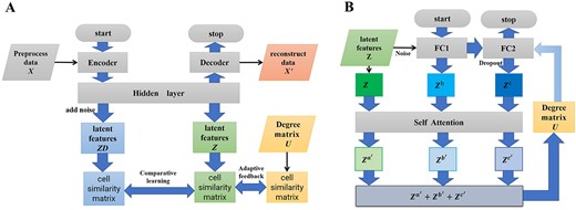
Module flowchart. (A) Deep DN flowchart. |$X$| gets latent features(|$ZD$| and |$Z$|) through with and without the noise-added network. Comparative learning is performed by constructing a cell similarity matrix by |$ZD$| and |$Z$|. The cell similarity matrix is also constructed for degree matrix |$U$| to supervise the cell similarity matrix constructed by |$Z$|.(B) Deep CN flowchart. The latent feature |$Z$| obtained by deep DN and the |$Z^b$|, |$Z^c$| obtained from the fully connected network with different noises are passed into the Self-Attention mechanism to get |$Z^{a^{\prime}}$|, |$Z^{b^{\prime}}$|, and |$Z^{c^{\prime}}$| and weight it to update U and optimize the network.
Adaptive feedback mechanism
Deep CN
In equation (10), |${w_{ij}} = \frac{{(1 + \sigma )(\sqrt{{{(Z{^{\prime}_i} - {C_j})}^2}} + 2\sigma )}}{{{{(\sqrt{{{(Z{^{\prime}_i} - {C_j})}^2}} + \sigma )}^2}}}$| is the adaptive loss weight for the network iterative optimization. |$C_j$| represents the clustering center of cluster |$j$|. |$u_{ij}$| represents the probability that the i-th cell is in the j-th cluster. |$Z^{a^{\prime}}$|, |$Z^{b^{\prime}}$|, and |$Z^{c^{\prime}}$| represents the latent features after Self-Attention. |$\sigma $| is a balance factor that controls the robustness of the network to outliers.
Evaluation metrics
To evaluate the validity of clustering methods for scRNA-seq datasets. We use datasets with cell labels, their cell labels are denoted as |$L = \{ L_1,L_2,\ldots ,L_R\}$|. These dataset labels were validated in previous research. Two common clustering evaluation metrics are often used to evaluate algorithm performance: normalized mutual information (NMI) [37], adjusted rand index (ARI) [38]. A larger value of them represents a higher degree of similarity between predicted labels and real labels. We set the prediction label |$L^{\prime} = \{ {L_1}^{\prime},{L_2}^{\prime},\; \ldots ,{L_R}^{\prime}\}$|.
In equation (14), |$V_{ij}$| represents the number of overlapping cells in |$L{^{\prime}_i}$| and |$L_j$|, |$a_i$| represents the number of |$i$| cell types in |$L^{\prime}$|, |$b_j$| represents the number of |$j$| cell types in |$L$|.
Results and discussion
Comparison with the clustering effect of other methods
To evaluate the clustering performance of scDASFK, we implement scDASFK on 16 real scRNA-seq datasets to get clustering results. The label information of these datasets is obtained through a large number of biological experiments while comparing with eight single-cell clustering methods with default parameters, including Celltree, Seurat, SHARP, SIMLR, scENA, scGMAI, scGAE and GraphSCC. These contrast methods are broadly classified into traditional machine learning methods and deep network-based methods. In addition, we evaluate each clustering model by two widely recognized clustering metrics (NMI, ARI) to demonstrate the performance of our model. All contrast methods used default parameters or settings recommended by the authors (The specific settings are described in the Supplementary Table S3). The input data for each clustering method is preprocessed the same and averaged 10 times.
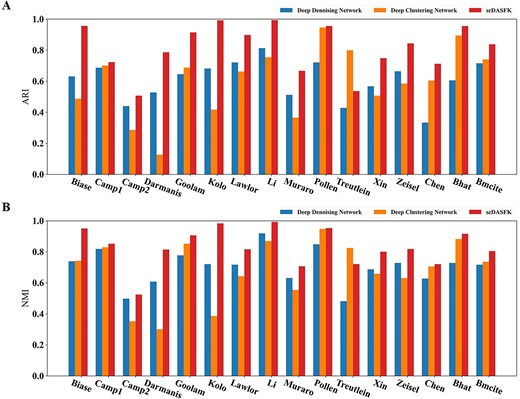
Figure 3A and B shows the effect of nine clustering methods on 16 scRNA-seq datasets. The detailed index values are shown in Supplementary Table S2. The index value in the figure decreases with the color from red to blue. The white area in the figure indicates that the clustering results cannot be obtained since time complexity or spatial complexity. From the figure, we observe that the overall effect of scDASFK on each data set is better than the other eight contrast methods. Specifically, scDASFK achieves the best NMI and ARI values on 14 datasets. Although the metric values of Biase and Treutlein datasets are not the highest, they are similar to the highest values and outperform most methods, probably because Biase and Treutlein datasets have the least amount of data, and deep models are not very friendly to small-scale datasets.
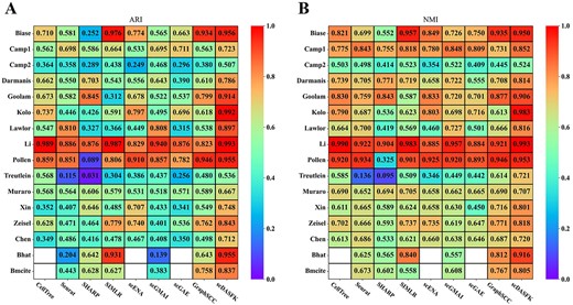
Clustering performance of scDASFK and eight other clustering methods. Kolo is the abbreviation of Kolodziejski dataset. Bhat is the abbreviation of Bhattacherjee dataset.
In order to show the clustering effect of scDASFK more clearly, we use T-SNE to project a real dataset into 2D space and visually compare the prediction results of nine methods. As shown in Figure 4, a dot represents a cell, and different colors represent different cell types. It is observed from the figure that different color clusters predicted by scDASFK in Camp1 dataset have obvious boundaries that can be clearly distinguished. However, in the other eight methods, only a few prediction cluster boundaries are clear for each method. The analysis shows that scDASFK better classifies cells that are close to each other into clusters.
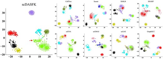
Visualization of prediction results from various clustering methods on Camp1 dataset.
Overall, the performance of scDASFK is superior to other contrast methods in both index values and visualization, which also indicates that scDASFK has better generalization ability.
Validity of potential characteristics
To verify the validity of the latent features of scDASFK, we visualize the latent features obtained by the four deep models of scGMAI, scGAE, GraphSCC and scDASFK on four datasets of Li (561 Cells), Lawlor (638 Cells), Muraro (3072 Cells) and Zeisel (3005 Cells) with different data scales and unknown cells and compare with the visualizations on the real datasets. As shown in Figure 5, different colors in the figure represent different real cell types. Compared with the real data and the other three deep models, scDASFK can better distinguishes the real cell clusters and make the boundaries between clusters obvious. In contrast, other methods tend to mix different cell types. For example, in Figure 5D, the real cell ‘alpha’ is clearly distinguished in scDASFK. In other methods, ‘alpha’ cells are mixed with other cells. The results in Figure 5 also shows scDASFK can learn useful information in real datasets while reducing the impact of noise on the data.
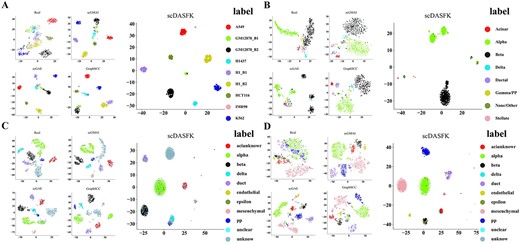
Visualization of latent features of scDASFK and three other deep models. (A) Li dataset, (B) Lawlor dataset, (C) Muraro dataset, (D) Zeisel dataset.
The Lawlor and Muraro datasets contain unknown cells. From their visualization results, we find that scDASFK can effectively distinguish between known real cell types and unknown cell types. To more clearly demonstrate the ability of scDASFK to differentiate unknown cells, we employed a common clustering internal evaluation: Silhouette Coefficient [40] to evaluate clustering performance. Silhouette coefficient values range from [−1, 1], with closer values to 1 indicating better clustering performance. We use the latent features and prediction results of unknown cells obtained by each deep model for experimental comparison. As shown in Figure 6, scDASFK achieves the optimal clustering performance, which illustrates that scDASFK has a good ability to discriminate unknown cells.
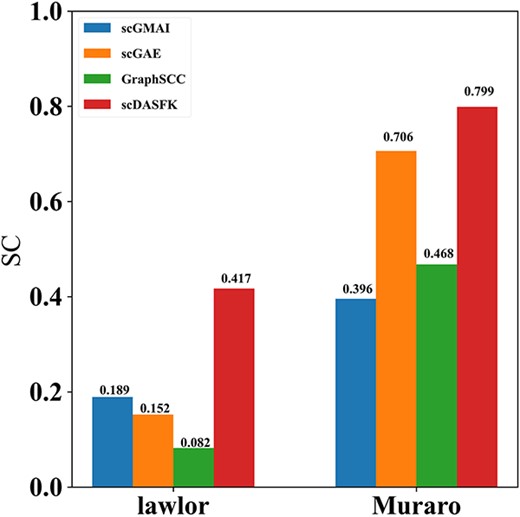
Silhouette coefficients of unknown cell latent features and predicted results obtained by scDASFK and three other deep models.
Dimension reduction ability
In order to verify that scDASFK can extract an effective low-dimensional representation of high-dimensional data, we remove all the deep model preprocessing processes and do not perform genetic screening on the data but directly reduce the dimension of the data through the model. For reduce the time cost, we use the public datasets Camp1, Camp2, Kolodziejski, Li, Xin and Zeisel with more than 500 cells and normalize and log them. We compare scDASFK with four classical dimension reduction methods of PCA [41], NMF [42], FastICA, UMAP [43] and three deep models of scGMAI, scGAE and GraphSCC. First, we use each method to reduce the gene dimension of the dataset to 50, 100 and 500 dimensions. Then, we use Gaussian clustering on these low-dimensional features to obtain the predicted cell type and calculate the NMI value. The number of Gaussian models is set to the number of real cell types. From Figure 7A, we find that the NMI value of scDASFK is higher than other dimensionality reduction methods in the average NMI value of different dimensions of each dataset, which means that scDASFK has better feature extraction ability, which is beneficial to realize cell clustering efficiently. From Figure 7B, it is seen that scDASFK is still optimal among the average NMI values of each method on all datasets, which indicates that the low-dimensional representation extracted by scDASFK has broad applicability to scRNA-seq data rather than for a single type dataset.
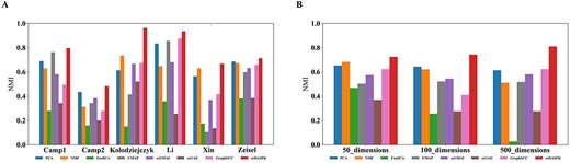
NMI for each dimensionality reduction method. (A) Average NMI of each method in each dataset in different dimensions.(B) Average NMI of each method on all datasets in each dimension.
Model stability
It is widely known that ‘dropout’ is considered as noise. Hence, to verify the denoising ability of scDASFK, we use the Li dataset in this experiment, which has high-performance indicators among various methods. Also, we used five random seeds to randomly select 20%, 30%, 40% and 50% of the nonzero values in the data and set them to zero, getting 20 different datasets. We compare scDASFK with eight other contrast methods on these datasets and use the average NMI to evaluate clustering performance. As shown in Figure 8, the NMI values of Celltree and scGMAI methods are almost close to the NMI values of scDASFK when the dropout is 40% and 50%, but the clustering performance of cellTree decreases significantly when the dropout is 20%. While scGMAI is relatively stable overall, the initial results are not optimal. With the increase of dropout, the scDASFK clustering performance decreases slightly, but scDASFK still obtains the highest NMI value, which indicates that different dropouts have less influence on the results of scDASFK. In a word, scDASFK has strong denoising ability and high stability under different levels of noise.
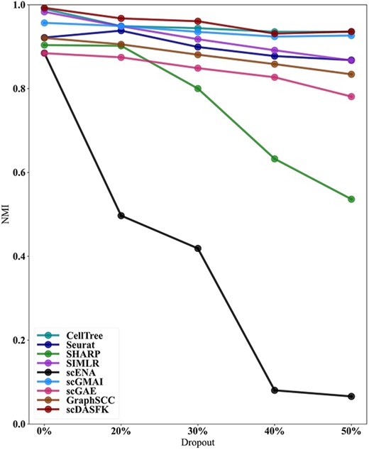
Changes in NMI values for each method on LI datasets with 20%, 30%, 40% and 50% dropout rates.
Cooperation between deep DN and deep CN
scDASFK has two core modules: deep DN and deep CN. The deep DN captures the cell correlation while reducing the effect of noise on the data by means of comparative learning. The deep CN further enhances the ability to capture useful information in low-dimensional features through self-attention and adaptive clustering loss function while clustering. In order to verify the cooperative relationship between deep DN and deep CN. We compare deep DN and deep CN as two new models with scDASFK. The deep DN removes the loss function brought by the adaptive feedback mechanism and performs k-means on the obtained latent features. The deep CN employs preprocessing to reduce the data dimension to the same dimension as the deep DN latent features with the input data. ARI and NMI are used to evaluate the clustering performance of each model. Figure 9 shows the scDASFK that combined them except Treutlein achieves the optimal clustering effect in all datasets. The ARI and NMI of the Treutlein dataset scDASFK are still higher than those of deep DN, which illustrates the promoting effect of deep CN on deep DN. The Treutlein dataset contains a small number of cells, and from the contrast experiment, it could be found that the Treutlein dataset did not have high index values in all methods, which illustrates that the Treutlein dataset contains a large amount of noise. The low cell number and high noise may make the process of contrast learning unable to accurately capture the potential characteristics of the Treutlein dataset, while the preprocessing process used by deep CN screens more valuable information about the genes. Therefore, the effect of scDASFK is inferior to that of deep CN, which also indicates the effectiveness of preprocessing in the scDASFK model.
Deep DN and deep CN and overall network scDASFK clustering performance.
Parameter analysis
Impact of noise type on scDASFK: the introduction of the noise is used to improve the anti-noise ability of the scDASFK model and enhance the stability of the model. In order to investigate the impact of noise type on scDASFK, we design the noise in the model as follows: (1) No noise is added to the model. (2) The dropout rate is set to 0%, 10%, 30%, 50%, 70% in the case of adding uniformly distributed noise. (3) Only add the dropout without adding uniform distribution noise, where the dropout rate is set to 10% corresponding to the best clustering effect. Figure 10A shows the average NMI and ARI values on different noise type settings. We observe that the scDASFK clustering results are better when two different noise types are added, but the excessive dropout rate also affects the clustering results. Therefore, we set to add uniformly distributed noise and dropout rate to 10%.
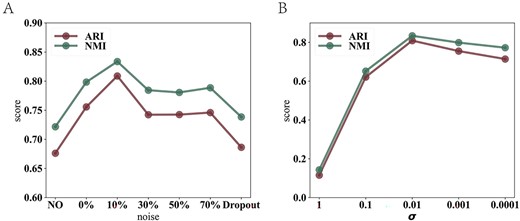
Parameter analysis. (A) Average NMI and ARI values with different noise parameters. NO represents do not add uniformly distributed noise and dropout, Dropout represents that only add the dropout without adding uniform distribution noise, and others represent the effect of the model with increasing dropout rate in the presence of uniformly distributed noise. (B) Average NMI and ARI values with different |$\sigma $| parameters.
Impact of balance factor |$\sigma $|: The balance factor |$\sigma $| as a hyperparameter as an adaptive loss function also affects the optimization update of scDASFK. To explore the impact of |$\sigma $| on scDASFK, we run scDASFK with the parameters 1, 0.1, 0.01, 0.001 and 0.0001. Figure 10B shows the average NMI and ARI values with different |$\sigma $| parameters. We can observe that the best clustering result is reached at |$\sigma $|=0.01 as the value of the |$\sigma $| parameter decreases, and then the clustering index gradually becomes lower. Therefore, we set |$\sigma $|=0.01.
Ablation study
Comparative learning, self-attention and adaptive feedback mechanism play an essential role in obtaining a good clustering effect. In this experiment, we analyze the impact of these components on the proposed model. Specifically, we delete different components to get three variants of scDASFK: scDASFK-AF (removing adaptive feedback mechanisms), scDASFK-SA (removing self-attention) and scDASFK-CL (removing comparative learning). Experiment results show the average ARI and NMI values on 16 datasets. As shown in Figure 11, we clearly find that scDASFK has the best performance, scDASFK-CL is almost close to the clustering performance of scDASFK and scDASFK-AF and scDASFK-SA have poor performance, which indicates that the interaction between adaptive feedback mechanisms and self-attention has a significant impact on the final results of the model. Comparative learning has little impact on the final effect of the model, and this may be since the fact that the adaptive feedback mechanism contains similar information between cells, which weakens the overall effect of comparative learning on the model. All in all, the three components are reasonable and effective, and their synergistic effect makes scDASFK the best results.
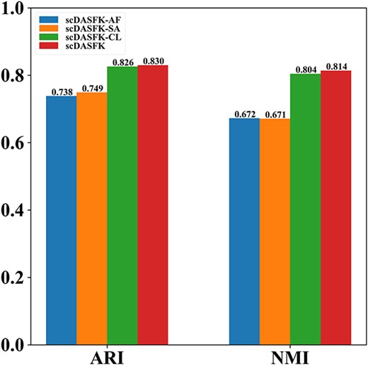
The clustering performance of remove each component in the designed architecture. scDASFK-AF represents the removal adaptive feedback mechanisms, scDASFK-SA represents the removal self-attention, and scDASFK-CL represents the removal comparative learning.
Implementation
scDASFK is implemented in Python 3 (version 3.6) using PyTorch (version 1.9.1+cu102). In the experiment part, all results are obtained by running 10 times. All experiments are conducted on Windows 10 with AMD Ryzen 7 4800H with Radeon Graphics 2.90 GHz, NVIDIA Geforce GTX 1650Ti GPU and 32 GB memory.
Conclusion
In this work, we propose a single-cell clustering method based on a deep model called scDASFK, which employs an advanced deep autoencoder with a denoising strategy based on comparative learning to preliminarily denoise the data and further extract valuable information from the denoised latent features by self-attention for clustering. Finally, an adaptive feedback mechanism is used to utilize the clustering results to supervise the deep autoencoder learning process. The above experimental results show that the scDASFK model proposed in this paper can better realize the clustering, dimensionality reduction and visualization of single-cell data, which also has a good discrimination ability for unknown cells. In the model learning process, it is necessary to give a certain number of cell clusters in advance, which makes the model has some limitations. Although the randomness of the deep network itself increases the search range of the optimal solution, it also makes the network have certain instability. Cell similarity network can obtain the similarity relationship between cells well, but it may not be able to obtain the global information of the data well. In the future, for better analysis of different scRNA-seq datasets, we will embed an imputation mechanism into scDASFK to better clean raw data and reduce data noise. We will also initialize the cell network using optimization algorithms and apply the graph-based deep model to capture global information about the data, and then use community detection algorithms to adaptively determine the number of cell clusters.
We develop a adaptive fuzzy clustering model based on the denoising autoencoder and self-attention mechanism called the scDASFK. It solves the problem that existing deep models often ignore the relationships between cells and require pretraining, which makes the models not widely applicable.
scDASFK uses a denoising autoencoder to obtain latent features of scRNA-seq data through comparative learning to discover relationships between cells. A self-attention mechanism to further reconstruct latent features to map scRNA-seq data to more appropriate features space and utilizes an adaptive clustering loss function for accurate clustering.
In order to avoid the disadvantage that the network requires pretraining, we introduce an adaptive feedback mechanism in the clustering process to guide comparative learning. Our scDASFK shows better performance than the other eight clustering methods on datasets of different species organization and scale and has good scalability for scRNA-seq data. It also has great potential for data dimensionality reduction and the discovery of new cell subtypes.
Data availability
The implementation of scDASFK is available at: https://github.com/LRX2022/scDASFK. The data that support the findings of this study are openly available at https://hemberg-lab.github.io/scRNA.seq.datasets/ and https://github.com/LRX2022/scDASFK/tree/main/dataset.
Funding
National Key Research and Development Program of China (2021YFE0102100); National Natural Science Foundation of China (62173145, 62173144, U19A2064, 61873001, 61890930-3); Anhui Provincial Natural Science Foundation (2008085QF294); National Natural Science Fund for Distinguished Young Scholars (61925305); University Synergy Innovation Program of Anhui Province (GXXT-2022-035).
Author Biographies
Yansen Su is an associate professor at the School of Artificial Intelligence, Anhui University. She is also with Institute of Artificial Intelligence, Hefei Comprehensive National Science Center, 5089 Wangjiang West Road, 230088 Hefei, China. Her research interests include bioinformatics, deep learning and multi-objective optimization.
Rongxin Lin is a master candidate at the School of Computer Science and Technology, Anhui University. His research interests include research of bioinformatics and deep learning.
Jing Wang is a PhD candidate at the School of Computer Science and Technology, Anhui University. Her research interests include research of bioinformatics and machine learning.
Dayu Tan is a lecturer with the Institute of Physical Science and Information Technology, Anhui University. He is also with Institute of Artificial Intelligence, Hefei Comprehensive National Science Center, 5089 Wangjiang West Road, 230088 Hefei, China. His research interests include machine learning, computer vision and data mining.
Chunhou Zheng is a professor at the School of Artificial Intelligence, Anhui University. His research interests include machine learning and bioinformatics.
References
