


Abstract
Natural products (NPs) and their derivatives are important resources for drug discovery. There are many in silico target prediction methods that have been reported, however, very few of them distinguish NPs from synthetic molecules. Considering the fact that NPs and synthetic molecules are very different in many characteristics, it is necessary to build specific target prediction models of NPs. Therefore, we collected the activity data of NPs and their derivatives from the public databases and constructed four datasets, including the NP dataset, the NPs and its first-class derivatives dataset, the NPs and all its derivatives and the ChEMBL26 compounds dataset. Conditions, including activity thresholds and input features, were explored to access the performance of eight machine learning methods of target prediction of NPs, including support vector machines (SVM), extreme gradient boosting, random forests, K-nearest neighbor, naive Bayes, feedforward neural networks (FNN), convolutional neural networks and recurrent neural networks. As a result, the NPs and all their derivatives datasets were selected to build the best NP-specific models. Furthermore, the consensus models, as well as the voting models, were additionally applied to improve the prediction performance. More evaluations were made on the external validation set and the results demonstrated that (1) the NP-specific model performed better on the target prediction of NPs than the traditional models training on the whole compounds of ChEMBL26. (2) The consensus model of FNN + SVM possessed the best overall performance, and the voting model can significantly improve recall and specificity.
Introduction
Nature is a valuable repository of novel bioactive entities. In the past 30 years, the percentage of new chemical entities inspired by natural products (NPs) and related molecules has risen to approximately 50%, 74% of which are concentrated in the field of antitumor [1]. NPs and their structural analogs have historically made significant contributions to the treatment of drugs, especially for cancer and infectious diseases. For example, quinine extracted from the bark of the Rubiaceae Cinchona tree plays an important role in the treatment of malaria [2]. Rosuvastatin, a blockbuster drug for the treatment of high cholesterol, mimics the pharmacophore of the NP mevastatin from the fungus Penicillium citrinum [3]. In general, the discovery of NPs profoundly affected the advances in biology and inspired drug discovery and therapy.
After entering the 21st century, technological and scientific advances, including analytical techniques, genome mining, engineering and cultivation systems, greatly promoted the NP-based drug discovery [4]. At the same time, a large amount of data on NPs have been produced. According to statistics, >120 different NPs databases and collections have been published and reused since 2000 [5]. There are many NP molecules, for example, COCONUT contains 885 447 NP molecules [6], however, the activity data are relatively lacking. The largest database of NP activity, NPASS, contains only 446 552 quantitative activity records [7].
The therapeutic activity of most drugs depends on their interaction with the targets, and about 95% of the targets are proteins [8]. Recent studies have shown that the NPs approved by the FDA or clinically investigated often target multiple proteins, which is called polypharmacology [9, 10]. Thus, systematically identifying the targets of NPs at the human proteome level would provide unexpected opportunities for the drug repositioning and reducing toxicity of NPs [11–13]. More activity data of NPs can be obtained using traditional experimental methods, but affinity chromatography and activity-based protein analysis experiments will inevitably produce high false alarm rates, and most traditional experimental assays for identifying targets of NPs are expensive and time-consuming [14–16]. Therefore, there is an urgent need of in silico prediction of the active targets for NPs to increase efficiency and save costs.
At present, many methods can be used for the target prediction of small molecules such as the reverse molecular docking [17], network pharmacology [9, 18] and similarity ensemble approach [19, 20]. Based on a large amount of public biological activity data, machine learning and deep learning algorithms have also been proposed and widely used to speed up the process of protein target identification for small molecules [21, 22]. Many of these virtual methods have also been practiced in the target prediction of NPs. For example, Begnini et al. [23] described how the core of macrocyclic NPs can serve as a high-quality in silico screening library for difficult-to-drug targets using reverse molecular docking strategy. Chen et al. [24] systematically explored the capacity of an alignment-based approach to identify the targets of large and flexible NPs and macrocyclic compounds. Cheng et al. [9, 25] developed statistical network models in order to link NPs to anti-cancer targets and proteins involved in aging-associated disorders. Cockroft et al. [26] developed a stacked ensemble approach for target prediction, StarFish, which used K-nearest neighbors (KNNs), multi-layer perceptron, random forest, logistic regression and model stacking methods and applied it to a NP set.
NPs are of great differences in many respects with synthetic molecules [3, 27–32], which can be roughly concluded as follows:
(i) Chiral carbon: NPs contain a much larger fraction of sp3-hybridized bridgehead atoms and chiral centers compared with synthetic small molecules, and NPs usually have higher steric complexity.
(ii) Diversity of ring systems: Only about 20% of the ring systems present in NPs can be found in trade drugs.
(iii) Element type: Drugs and combinatorial molecules tend to contain more nitrogen-, sulfur- and halogen- containing groups, while NPs have more oxygen atoms.
(iv) Functional group: NPs differ significantly from synthetic drugs and combinatorial libraries in the ratio of aromatic ring atoms, the number of solvated hydrogen-bond donors and acceptors.
(v) Molecular properties: NP libraries have a wider range of molecular properties, such as molecular mass and octanol–water partition coefficient, compared with synthetic and combinatorial counterparts.
To our knowledge, none of the current methods specifically distinguish between NPs and synthetic molecules to make target prediction for NPs, nor there has been a large-scale comparison of methods of NP target prediction. For this reason, we hope to use multiple algorithms to build the NP-specific models based on the activity data of NPs and their derivatives, which are defined as naturally occurring compounds that have been chemically modified or a collection of the purely synthetic medicinal compounds inspired by natural compounds [33–36].
In the present study, several NPs specific datasets and the all compounds’ dataset from CHEMBL26 were constructed to build a variety of machine learning classification models for the evaluation of the difference between NP-specific datasets and traditional mixed datasets on the target prediction task of NPs. A total of eight machine learning algorithms were used here, including standard feedforward neural networks (FNN), convolutional neural networks (CNN), recurrent neural networks (RNN), support vector machines (SVM), naive Bayes (NB), KNN, random forests (RF) and extreme gradient boosting (XGBoost).
Methods
Data construction
The original NPs were extracted from COCONUT. The derivatives were mined from BindingDB [37], ChEMBL [38] and PubChem Bioassay [39] according to the definition that derivatives were chemically modified from natural compounds. We define compounds that are modified directly from NPs as first-class derivatives, and the rest obtained by remodifying from derivatives along with first-class derivatives are all derivatives of NPs. More detailed information can be found in the Data Collection section and Figure S3 of Supporting information.
To obtain high-quality training datasets, only assays measured in IC50, Ki or Kd and unit of nM against a single protein target were considered [40]. Specifically, we kept the biochemical assays which were annotated with a confidence score of ≥4 [41]. Afterward, the molecules with quantitative activity records were discretized into four class categories based on activity thresholds, namely active, weak active, inactive and weak inactive as described by Mayr et al. [21]. The activity thresholds of the labels are shown in Table 1. The active and inactive data were used as positive and negative samples for training a model, and compounds labeled with weak active or weak inactive were additionally used as weakly data to discuss the impact of activity thresholds. To guarantee the quality of the model, the compound-target pairs with ambiguous labels were discarded and the targets with <100 molecules or <3 active/inactive molecules were further removed [42].
Division criteria of threshold
| Label | Thresholds in −log10(M) |
|---|---|
| Active | ≥5.5 |
| Weak active | >5.0 and <5.5 |
| Inactive | ≤4.5 |
| Weak inactive | >4.5 and <5.0 |
| Label | Thresholds in −log10(M) |
|---|---|
| Active | ≥5.5 |
| Weak active | >5.0 and <5.5 |
| Inactive | ≤4.5 |
| Weak inactive | >4.5 and <5.0 |
Following the above steps, we built eight datasets from the ChEMBL26 as training sets, and for a better distinction, we added the label ‘Weak’ to the abbreviation of datasets with weakly data to distinguish from the datasets without weakly data: (1) the NPs dataset without weakly data (NPs), (2) the NPs and its first-class derivatives dataset without weakly data (NPs + Der1), (3) the NPs and all its derivatives dataset without weakly data (NPs + DerALL), (4) whole compounds dataset from ChEMBL26 without weakly data (ChEMBL26), (5) the NPs dataset with weakly data (Weak NPs), (6) the NPs and its first-class derivatives dataset with weakly data (Weak NPs + Der1), (7) the NPs and all its derivatives dataset with weakly data (Weak NPs + DerALL) and the (8) whole compounds dataset from ChEMBL26 with weakly data (Weak ChEMBL26).
Furthermore, an external validation set was constructed using the ChEMBL29, the NPASS, BindingDB and PubChem Assays, which removed the target-compound pairs overlapping with the training dataset.
Molecular fingerprints
Three binary fingerprints, extended connectivity fingerprints (ECFP), functional connectivity fingerprints (FCFP) and molecular access system (MACCS) were used as chemical descriptors in this study. MACCS is a 166-bit fingerprint based on a well-defined dictionary of substructure(MACCS keys) [43]. ECFP and FCFP descriptors are substructure fingerprints based on the Morgan algorithm [44], which represent feature sets of circular atom neighborhoods by compiling the surrounding environment of atoms iteratively. The differences between ECFP and FCFP are the atomic characteristics during initialization. The initial identifier of an atom in ECFP is obtained from several properties of the atom itself, whereas FCFP uses functional group types before substructures are enumerated. We compare the prediction performance of each fingerprint and the combination of them. Fingerprint representations are generated using the RDKit implementation of MACCS (166-bit), 2048-bit ECFP6 (radius = 3) and 2048-bit FCFP6 (radius = 3). The combinations of different fingerprints refer to connecting the bit string of each fingerprint, for example, a combination of 166-bit MACCS and 2048-bit ECFP6 had 2214 bits.
Cluster cross-validation
Cluster cross-validation is today’s popular data-partitioning scheme that which compounds are clustered based on the chemical similarity before dividing the training and testing sets [45]. In the experiment, we conducted 3-fold cross-validation with compounds clustered in advance to evaluate the performance of the model. To prevent similar data points from falling into the training set and the test set at once, all of the molecules were first clustered by the single linkage algorithm. Jaccard distance using binarized Morgan fingerprints with a radius of 2 was employed as the metric between any two compounds and the minimum distance was set to 0.3. In the next step, molecules belonging to the same cluster were randomly assigned to one of the 3-folds. We also compared the performance of the cluster cross-validation and random cross-validation (see Table S12).
Nested cluster cross-validation
To get a fair evaluation, nested cross-validation was performed for parameter tuning. For nested cross-validation, training data are split into two portions: inner and outer portions. Different hyperparameter combinations were attempted in the inner loop to evaluate which hyperparameter can achieve the best performance. Hyperparameters and the performance comparison of RF and XGBoost with default parameters and selected hyperparameter can be found in Table S1, S2 and Table S9. Then, the selected hyperparameter is employed in the outer loop to get a model for each fold, which could avoid the hyperparameter selection bias of performance evaluation. The area under the curve (AUC) of the receiver operating characteristic was calculated here for assessing model performance. For each hyperparameter combination, we obtained the AUC values from the inner rings and the mean AUC values of two inner loops were adopted as the criteria to select the optimal hyperparameter combination for the corresponding outer ring. At last, we summarized the AUC values of three outer loops by calculating their average values to obtain the most realistic results of model performance evaluation. At the same time, the best optimal hyperparameter combination was confirmed by calculating the mean AUC values of the six inner loops of the nested cluster cross-validation [22] and then used to train the final models on all data.
Machine learning methods
We compared the prediction performances of eight machine learning architectures for NP target fishing, including three deep learning methods (FNN, CNN and RNN) and five traditional machine learning approaches (SVM, XGBoost, RF, KNN and NB).
NB has been widely used in target prediction and is included as a baseline method. Particularly, SVM and KNN are typical classification methods based on similarity, RF and XGBoost are representative classification methods based on feature, while XGBoost implements gradient tree boosting. Deep learning methods have recently garnered significant attention in target fishing, and three representative architectures of deep neural networks are considered in this study. Among them, FNN follows the standard feedforward architecture and takes vectorial inputs, CNN has advantages in image processing and mimics its traits in the convolutional layers and RNN process the sequence data with cyclic connections using memory blocks. The details of each algorithm were provided in the Supporting information. The overall workflow to assess the predictive performances of the machine learning algorithms on different datasets is shown in Figure 1.
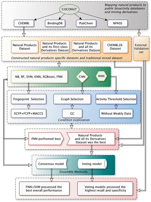
The overall workflow to assess the predictive performances of the machine learning algorithms on different datasets.
Results and Discussion
Dataset
Eight different datasets and an external validation set were prepared for evaluating the NP target prediction models. The statistic of each dataset can be found in Table 2. A total of 899 single protein targets with varying numbers of data points were identified for ChEMBL26. The targets contain between 100 and 7086 unique compounds with a mean of 795, a median of 410 and the first quartile of 191. The smallest dataset, NPs, contained 26 targets. The min, max, mean, median and the first quartile of data points of NPs were 100, 592, 174, 148 and 122, respectively. The detailed information is provided in the Supplement Materials.
The number of targets, compounds and bioactivities of each dataset
| Datasets | Targets_number | Compound_number | Bioactivity_number |
|---|---|---|---|
| ChEMBL26 | 899 | 458 198 | 714 438 |
| NPs + DerALL | 470 | 97 706 | 164 195 |
| NPs + Der1 | 150 | 18 493 | 30 543 |
| NPs | 26 | 3052 | 4521 |
| Weak ChEMBL26 | 1084 | 522 416 | 863 677 |
| Weak NPs + DerALL | 585 | 121 729 | 219 793 |
| Weak NPs + Der1 | 211 | 26 279 | 46 236 |
| Weak NPs | 37 | 4176 | 7250 |
| External validation set | 666 | 7205 | 10 776 |
Fingerprint selection
Feature selection is a key step in machine learning. For small molecules, the SMILS strings, molecular fingerprints and molecular graphs can be used as input features. Most machine learning algorithms use molecular fingerprints as input [22, 26, 46, 47]. With the progress of deep learning algorithms, the construction of CNN models using molecular graphs as input features and RNN models using SMILES strings as input features have also shown good performance [21]. Therefore, in this work, the molecular graphs and SMILES strings are adopted for CNN and RNN, respectively, whereas the rest six algorithms take molecule fingerprints as input. Generally, the choice of molecular fingerprints will affect the performance of a ligand-based target prediction model [47]. Here, we estimated three fingerprints (ECFP6, FCFP6 and MACCS) and combinations of them (ECFP6 + FCFP6, ECFP6 + MACCS, FCFP6 + MACCS and ECFP6 + FCFP6 + MACCS) using six machine learning methods (FNN, SVM, RF, KNN, NB and XGBoost) on six datasets, including NPs, NPs + Der1, ChEMBL26, Weak NPs, Weak NPs + Der1 and Weak ChEMBL26. The intersection targets of NPs, NPs + Der1 and ChEMBL26, which include 26 targets, were taken into comparison. Accordingly, 37 targets of Weak NPs, Weak NPs + Der1 and Weak ChEMBL26 were discussed as the intersection. The results of ChEMBL26 are listed in Table 3, and the result of the other five datasets can be found in Supplementary Tables S3–S7 available online at https://dbpia.nl.go.kr/bib. As shown in Table 3, the averaged AUC values of models using ECFP6 + MACCS+FCFP6 ranked first at four out of six machine learning methods. In terms of the other five datasets, ECFP6 + MACCS+FCFP6 performed best on Weak NPs + Der1 (Supplementary Table S6 available online at https://dbpia.nl.go.kr/bib) and Weak ChEMBL26 (Supplementary Table S7 available online at https://dbpia.nl.go.kr/bib). The poor performances of ECFP6 + MACCS+FCFP6 on NPs (Supplementary Table S3 available online at https://dbpia.nl.go.kr/bib), Weak NPs (Supplementary Table S4 available online at https://dbpia.nl.go.kr/bib) and NPs + Der1 (Supplementary Table S5 available online at https://dbpia.nl.go.kr/bib) were possibly due to the small dataset which brought about a relatively unobvious, unstable and biased evaluation. In addition, no matter which dataset, the combination of different fingerprints always performed better than a particular fingerprint. Overall, using the combined fingerprints, which contain more molecular properties, yields better performance. Therefore, the ECFP6 + MACCS+FCFP6 was picked out as the optimal fingerprint combination and was selected as the input feature in the following training work.
Performance comparison of different target prediction methods on ChEMBL26; the table gives the means and SDs of AUC values for the compared algorithms and feature categories or input types; the top 1 AUC values were marked as bold text
| FNN | RF | SVM | XGBOOST | KNN | NB | |
|---|---|---|---|---|---|---|
| ECFP6 | 0.869 ± 0.072 | 0.890 ± 0.061 | 0.889 ± 0.072 | 0.869 ± 0.071 | 0.828 ± 0.108 | 0.840 ± 0.079 |
| FCFP6 | 0.871 ± 0.080 | 0.884 ± 0.071 | 0.892 ± 0.047 | 0.876 ± 0.069 | 0.825 ± 0.109 | 0.842 ± 0.065 |
| MACCS | 0.878 ± 0.063 | 0.884 ± 0.062 | 0.871 ± 0.059 | 0.877 ± 0.063 | 0.827 ± 0.080 | 0.779 ± 0.076 |
| ECFP6 + FCFP6 | 0.880 ± 0.074 | 0.893 ± 0.062 | 0.908 ± 0.047 | 0.885 ± 0.062 | 0.832 ± 0.110 | 0.847 ± 0.069 |
| ECFP6 + MACCS | 0.888 ± 0.053 | 0.896 ± 0.062 | 0.898 ± 0.065 | 0.889 ± 0.059 | 0.838 ± 0.113 | 0.836 ± 0.067 |
| FCFP6 + MACCS | 0.877 ± 0.065 | 0.900 ± 0.063 | 0.902 ± 0.045 | 0.891 ± 0.068 | 0.838 ± 0.105 | 0.840 ± 0.060 |
| ECFP6 + FCFP6 + MACCS | 0.880 ± 0.065 | 0.900 ± 0.059 | 0.911 ± 0.046 | 0.892 ± 0.064 | 0.838 ± 0.111 | 0.844 ± 0.062 |
Graph selection
In the case of CNN, the ConvMolFeaturizer and WeaveFeaturizer were compared as input features, which are referred to as GC and Weave, respectively. The detailed comparison results are listed in Table 4. According to AUC values, the GC performed better than Weave on the six datasets. Thus, GC was applied in the follow-up works.
The means and SDs of AUC values of GC and Weave for the datasets with and without weakly data
| Dataset | GC | Weave |
|---|---|---|
| NPs | 0.824 ± 0.081 | 0.794 ± 0.072 |
| NPs + Der1 | 0.855 ± 0.065 | 0.839 ± 0.061 |
| ChEMBL26 | 0.882 ± 0.056 | 0.855 ± 0.055 |
| Weak NPs | 0.747 ± 0.111 | 0.712 ± 0.098 |
| Weak NPs + Der1 | 0.790 ± 0.072 | 0.780 ± 0.065 |
| Weak ChEMBL26 | 0.834 ± 0.075 | 0.814 ± 0.058 |
Activity threshold selection
In some cases, existing research use traditional machine learning with weakly active data removed, and deep learning is considered to distinguish the data in the weakly active region [21, 40, 48]. Since NPs often interact with multiple targets in a weak-bonded way [49–52], it is necessary for NPs to discuss the effects of weak activity data. Therefore, we used two dataset partitioning methods to explore whether it is better to directly select a certain threshold value or exclude the weakly data points. The results of eight algorithms (FNN, GC SVM, RF, KNN, NB, XGBoost and LSTM) were displayed as a boxplot in Figure 2. The orange line in each boxplot represents the median AUC values of the eight models. It can be seen from Figure 2 that the models excluding weakly active data (blue boxes) generated significantly higher median AUC values (orange lines in the boxes) than the models containing weakly active data (green boxes). Without special instructions, all models in the late evaluations were defaulted to use the dataset excluding weakly active data.
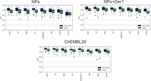
The effects of weakly data and no weakly data on the performance of NPs, NPs+Der1 and ChEMBL26.
Large-scale comparison
After determining the input characteristics and activity thresholds on a small range of crossover targets (26 targets for datasets without weakly data and 37 targets for datasets with weakly data), we compared the training results of eight algorithms on a larger benchmark of four datasets with whole targets (ChEMBL26 with 899 targets, NPs + DerALL with 470 targets, NPs + Der1 with 150 targets and NPs with 26 targets). The means and standard deviations (SDs) of AUC values of the eight algorithms in the four datasets are shown in Table 5. It can be found that FNN performed best with the highest averaged AUC value (marked as bold text in Table 5) in three datasets, which is consistent with the work of Mayr et al. [21], that deep learning methods significantly outperform all competing methods. In addition, we found that FNN, GC, SVM and RF performed stable with an averaged AUC value >0.8, and LSTM, XGBoost and KNN have poor performance in small datasets (NPs and NPs + Der1), while NB always worked poorly in all datasets. We also trained models on ChEMBL29 benchmark with more hyperparameters, and the results were similar to the models constructed using the ChEMBL26 database, see Table S10, S11.
The means and SDs of AUC values of the eight methods in the four datasets, the top 1 AUC values were marked as bold text
| NPs | NPs + Der1 | NPs + DerALL | ChEMBL26 | |
|---|---|---|---|---|
| FNN | 0.811 ± 0.083 | 0.854 ± 0.109 | 0.890 ± 0.099 | 0.884 ± 0.091 |
| RF | 0.825 ± 0.098 | 0.838 ± 0.130 | 0.873 ± 0.106 | 0.866 ± 0.106 |
| SVM | 0.835 ± 0.080 | 0.837 ± 0.140 | 0.871 ± 0.127 | 0.856 ± 0.134 |
| LSTM | 0.667 ± 0.087 | 0.772 ± 0.117 | 0.859 ± 0.110 | 0.850 ± 0.105 |
| GC | 0.824 ± 0.081 | 0.834 ± 0.113 | 0.851 ± 0.115 | 0.842 ± 0.110 |
| XGBoost | 0.793 ± 0.115 | 0.816 ± 0.134 | 0.841 ± 0.123 | 0.835 ± 0.126 |
| KNN | 0.761 ± 0.109 | 0.785 ± 0.125 | 0.819 ± 0.124 | 0.815 ± 0.115 |
| NB | 0.782 ± 0.109 | 0.717 ± 0.161 | 0.737 ± 0.163 | 0.739 ± 0.159 |
Statistics of the better and poorer targets of NPs + DerALL, NPs + Der1 and NPs compared with the same targets in ChEMBL26
| 26 targets | 150 targets | 463 targets | ||||
|---|---|---|---|---|---|---|
| Better_number | Poorer_number | Better_number | Poorer_number | Better_number | Poorer_number | |
| FNN | ||||||
| NPs | 2 | 24 | ||||
| NPs + Der1 | 11 | 15 | 50 | 100 | ||
| NPs + DerALL | 15 | 11 | 82 | 68 | 248 | 215 |
| GC | ||||||
| NPs | 12 | 14 | ||||
| NPs + Der1 | 12 | 14 | 55 | 95 | ||
| NPs + DerALL | 17 | 9 | 85 | 65 | 251 | 212 |
| SVM | ||||||
| NPs | 4 | 22 | ||||
| NPs + Der1 | 9 | 17 | 46 | 104 | ||
| NPs + DerALL | 12 | 14 | 79 | 71 | 245 | 218 |
| RF | ||||||
| NPs | 8 | 18 | ||||
| NPs + Der1 | 11 | 15 | 47 | 103 | ||
| NPs + DerALL | 12 | 14 | 72 | 78 | 230 | 233 |
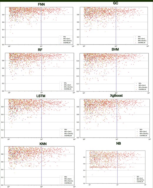
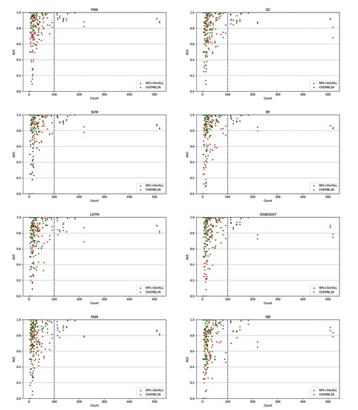
The relationship between the amount of data under the target and AUC value. The abscissa is the amount of data under the target point, and the ordinate is the AUC value. The blue dotted lines at data size value of 1000 differentiate models with stable or unstable results.
We also discussed the target prediction results of a particular algorithm across different datasets. To be fair, the intersection targets of different datasets were taken for comparison furtherly. For example, there were 26 targets of ChEMBL26, NPs + DerALL and NPs + Der that intersected with NPs; 150 targets of ChEMBL26 and NPs + DerALL that intersected with NPs + Der1 and 463 targets of ChEMBL26 that intersected with NPs + DerALL. Based on the AUC value, we compared the performance of NPs + DerALL, NPs + Der1 and NPs with ChEMBL26 on each target, and then the number of targets with higher AUC values than ChEMBL26 was calculated as the Better Number, while those with lower or equal AUC values were called Poorer Number and Equal Number, respectively. Table 6 shows the results of FNN, GC, SVM and RF, and the results of KNN, NB, XGBoost, and LSTM can be found in Supplementary Table S8 available online at https://dbpia.nl.go.kr/bib. For FNN, among the 26 NPs targets, 2 targets had higher AUC values than that of ChEMBL26. This number increased from 2 to 12 on NPs + Der1 and then increased to 15, which was more than half of 26 NPs targets. For 150 targets of NPs + Der1, a greater number of targets (50) presented a better AUC value. And 83 out of 150 targets of NPs + DerALL exceeded the ChEMBL26. It should be noted that the NPs + DerALL dataset had more better targets than ChEMBL26 on three out of four stable machine learning methods. From the above results, we can see that NPs + DerALL, NPs + Der1 and NPs with less data than ChEMBL26 can still obtain higher-level models, which shows the great potential of NP-specific datasets.
Previous works showed that the number of training sets increased, the performance of the model increased [21, 53, 54]. We also investigated the correlation between dataset size and performance. The scatter plots of data sizes against AUC values were drawn for all models. As shown in Figure 3, from left to right, the distribution of AUC was getting closer and closer to the top, demonstrating that the larger training set leads to better predictions. This is consistent with previous work [55–59]. Especially, when the amount of data reaches 103–104, the AUC values were concentrated at the range of 0.8~1, which was a relatively high and stable level. In general, NPs (green points) and NPs + Der1 (blue points) were difficult to achieve a stable data size, and the NPs + DerALL (yellow points) met this requirement and thus got better performance than ChEMBL26. Therefore, we believe that, when the datasets are sufficient in the future, NP-specific datasets will have the potential of getting a better model for NP target prediction rather than the models built with a hybrid dataset of all ChEMBL molecules which have more data.
The number of targets, molecules and bioactivity measurements in the intersection of external validation set
| Targets_number | Compound_number | Bioactivity_number |
|---|---|---|
| 192 | 4516 | 5824 |
| Targets_number | Compound_number | Bioactivity_number |
|---|---|---|
| 192 | 4516 | 5824 |
The number of targets, molecules and bioactivity measurements in the intersection of external validation set
| Targets_number | Compound_number | Bioactivity_number |
|---|---|---|
| 192 | 4516 | 5824 |
| Targets_number | Compound_number | Bioactivity_number |
|---|---|---|
| 192 | 4516 | 5824 |
The statistical of better, poorer and equal targets based on 13 targets (with more than 100 compounds) in the external validation set
| Optimal number of targets in NPs + DerALL models | |||
|---|---|---|---|
| Better_number | Equal_number | Poorer_number | |
| FNN | 8 | 2 | 3 |
| GC | 6 | 1 | 6 |
| LSTM | 8 | 1 | 4 |
| SVM | 6 | 2 | 5 |
| RF | 5 | 2 | 6 |
| XGBOOST | 6 | 1 | 6 |
| KNN | 5 | 1 | 7 |
| NB | 7 | 1 | 5 |
| Optimal number of targets in NPs + DerALL models | |||
|---|---|---|---|
| Better_number | Equal_number | Poorer_number | |
| FNN | 8 | 2 | 3 |
| GC | 6 | 1 | 6 |
| LSTM | 8 | 1 | 4 |
| SVM | 6 | 2 | 5 |
| RF | 5 | 2 | 6 |
| XGBOOST | 6 | 1 | 6 |
| KNN | 5 | 1 | 7 |
| NB | 7 | 1 | 5 |
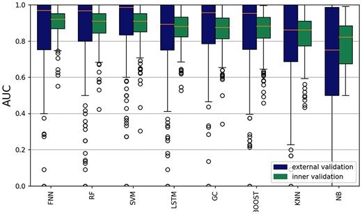
The AUC values of the model itself versus external validation.
External validation
Several studies demonstrated the performance of cross-validation differences between in-sample and out-of-sample test pairs [60, 61]. To better evaluate the models, the external validation set without training samples was built and used on the final models which were trained on all data. Considering that most of the targets of NPs and NPs + Der1 have very little data of the training and external validation sets, and the data were distributed unevenly, only the performance of NPs + DerALL and ChEMBL26 were compared on the external validation set.
First, the evaluation results of the internal validation based on nested cluster cross-validation were compared with that of external validation to evaluate the generalization capacity of our models. The result of NPs + DerALL is displayed in Figure 4. As shown in the boxplot, the results from the internal (green boxes) and external validation (blue boxes) of those models displayed comparable performance, and most of the time, the external validation possessed higher median AUC values (orange lines in the boxes) than the internal validation. Therefore, our training models possessed good robustness.
Next, we evaluated whether the NP specificity models built with NPs + DerALL performed better for the NP target prediction than traditional models with all mixed molecules of ChEMBL26. Due to the data size limitation, the AUC value was unable to be calculated for some targets, then the intersection targets of NPs + DerALL and ChEMBL26 with complete estimate values were picked out. In the end, 192 targets were selected (Table 7) and the details of those 192 targets can be found in Supplement Materials.
Considering that the size of the external validation set also had a significant impact on the model estimate, the correlation of the data distribution and the AUC values were further analyzed and these are displayed in Figure 5. It was shown when the data volume of a target in the external validation set was >100, the performance of most models could reach a reliable level with an AUC value of >0.8. On the contrary, the results were very messy when the amount of the external validation set was <100. Therefore, only targets with >100 compounds were explored in the following discussion.
The relationship between the data size of the external validation set and the performance of the eight different models. The blue dotted lines at data size value of 100 differentiate models with stable or unstable results.
Table 8 shows a chart of the numbers of better, poorer and equal targets with a data size of >100. In this case, there were relatively more targets of NPs + DerALL performing better than ChEMBL26. Besides, the means and SDs of the AUC value of eight methods for those targets with external data size >100 were tallied up and these are listed in Table 9. The FNN and LSTM obtained better performances on NPs + DerALL and the FNN model of NPs + DerALL performed best with the highest AUC value of 0.944. For other methods, the averaged AUC values on NP + DerALL were very close to the results on ChEMBL26. In summary, the NP-specific models (NPs + DerALL) are able to produce a better predictive ability of target prediction for NPs and their derivatives.
The means and SDs of the AUC values of eight methods for the NPs + DerALL and ChEMBL26
| NP + DerALL | ALL | |
|---|---|---|
| FNN | 0.944 ± 0.044 | 0.933 ± 0.057 |
| GC | 0.911 ± 0.085 | 0.918 ± 0.061 |
| LSTM | 0.910 ± 0.073 | 0.883 ± 0.101 |
| SVM | 0.929 ± 0.070 | 0.933 ± 0.061 |
| RF | 0.931 ± 0.066 | 0.935 ± 0.063 |
| XGBOOST | 0.915 ± 0.081 | 0.913 ± 0.083 |
| KNN | 0.888 ± 0.078 | 0.902 ± 0.069 |
| NB | 0.879 ± 0.104 | 0.874 ± 0.110 |
Consensus model
Ensemble methods by combining multiple learners can often obtain significantly better generalization performance than a single learner [62–65]. Therefore, we combined eight different models to build consensus models for NP target prediction and to evaluate their performance on external validation sets. The average probability was used as the predicted score for two-algorithms-combined (28 in total) or three-algorithms-combined (56 in total) consensus models [66, 67]. Eight measurements of performance, including AUC, the area under the PR curve (AP), accuracy, precision, specificity, F1-score, kappa and recall, were used to estimate the overall performance of different consensus models in target prediction jobs. The partial results are shown in Figure 6, and the rest are displayed in Supplementary Figure S1 available online at https://dbpia.nl.go.kr/bib. The full evaluation results of the consensus models can be found in the Supplement Materials.
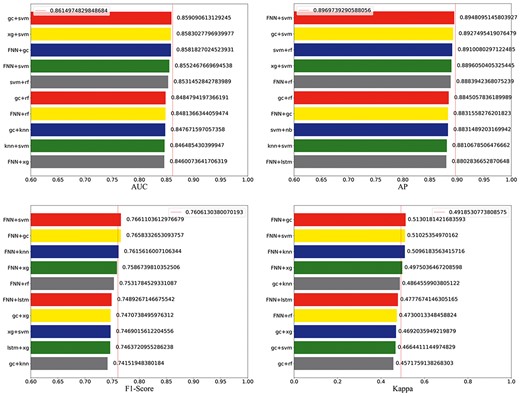
The values of AUC, AP, F1-score and kappa of two combined models. The red standard line represents the best value of single models.
For the two-algorithms-combined models, the GC + SVM ranked first at the AUC. FNN + SVM ranked first at AP and F1- score, FNN + GC ranked first at the kappa and accuracy, FNN + KNN ranked first at the precision and specificity, while LSTM + XGBoost ranked first at recall. Therefore, different consensus models have their advantages. But from a comprehensive view, five out of eight indicators (AP, kappa, accuracy, precision and F1-score) of the FNN + SVM ranked first or second, which indicated that FNN + SVM had the best overall performance. For the three-algorithms-combined models (Supplementary Figure S2 available online at https://dbpia.nl.go.kr/bib), the FNN + GC + XGBoost performed best at five indicators (accuracy, AP, precision, F1-score and kappa). But, the best two-algorithms-combined models were superior to the best three-algorithms-combined model at six indicators excluding the accuracy and AP. So overall, the FNN + SVM possessed the best overall performance, and this consensus model indeed improved the score of multiple evaluation methods than a single model and thereby highlights the comprehensive advantages of ensemble methods for NP target fishing.
Multi-voting method
The voting method is another ensemble technique. We use the voting method to predict targets for NPs by combining the eight algorithms. The results are listed in Table 10. If we considered 1 vote (Vote_1 scheme), a positive label was given only if one or more models were giving a positive label. And the Vote_8 scheme required all eight models to label positive. Although the voting model performed poorly on most metrics, the vote_1 model had the highest recall of 0.927, which is a good choice when we want to find more candidate targets. On the other side, the Vote_8 model had the highest specificity with a massive improvement from 0.725 (the best of the single model) to 0.923, which demonstrated its great ability to raise the true negative rate. In another word, if it aimed to accurately exclude targets without effect on molecules, more votes were necessary.
Voting results and single model results of eight models on accuracy, precision, specificity, balanced average (F1-score), consistency test index (kappa) and recall; the top 1 of each indicators were marked as bold text
| Accuracy | Recall | Precision | Specificity | F1-score | Kappa | |
|---|---|---|---|---|---|---|
| Vote_1 | 0.734820 | 0.927357 | 0.690474 | 0.334298 | 0.768811 | 0.257488 |
| Vote_2 | 0.756605 | 0.863349 | 0.705754 | 0.457933 | 0.753761 | 0.327965 |
| Vote_3 | 0.768086 | 0.824571 | 0.721773 | 0.532612 | 0.746595 | 0.363039 |
| Vote_4 | 0.785580 | 0.794663 | 0.720453 | 0.606143 | 0.731923 | 0.395788 |
| Vote_5 | 0.784754 | 0.752909 | 0.722685 | 0.683765 | 0.712288 | 0.425853 |
| Vote_6 | 0.786689 | 0.706961 | 0.727658 | 0.760024 | 0.691929 | 0.451502 |
| Vote_7 | 0.777391 | 0.640642 | 0.730498 | 0.837807 | 0.657155 | 0.442357 |
| Vote_8 | 0.727814 | 0.518230 | 0.707729 | 0.923482 | 0.570414 | 0.374407 |
| FNN | 0.798308 | 0.791062 | 0.767744 | 0.725392 | 0.760613 | 0.491853 |
| KNN | 0.729326 | 0.688061 | 0.700937 | 0.657092 | 0.659602 | 0.320299 |
| XGBoost | 0.786030 | 0.803387 | 0.737362 | 0.615127 | 0.744092 | 0.419844 |
| NB | 0.720282 | 0.662418 | 0.690309 | 0.643922 | 0.643178 | 0.280391 |
| RF | 0.762731 | 0.760221 | 0.690735 | 0.598778 | 0.697785 | 0.353804 |
| SVM | 0.765061 | 0.778616 | 0.718526 | 0.581766 | 0.720179 | 0.359531 |
| GC | 0.792923 | 0.776271 | 0.728246 | 0.693327 | 0.733131 | 0.445779 |
| LSTM | 0.767079 | 0.768647 | 0.726224 | 0.620660 | 0.722073 | 0.386801 |
Conclusions
NPs are valuable resources of drugs, and the study of the activity of NPs, especially the discovery of specific targets, is very important for the development of NPs. With the increase of data, various algorithms have been successfully used in molecular target prediction, but considering the obvious differences between the characteristics of NPs and synthetic molecules, it is significantly necessary to construct prediction models that are specific for NPs. Therefore, we collected the activity data of NPs and their derivatives to build three specific datasets of NPs, NPs, NPs + Der1 and NPs + DerALL. Multiple machine learning methods, including SVM, XGBoost, RF, KNN, NB, FNN, CNN and RNN, were used to construct NP-specific target prediction models and were then compared with the traditional models constructed by ChEMBL26.
We first discussed the effects of the input features, activity thresholds on different datasets with multiple algorithms. The results showed that the combination of ECFP6 + MACCS+FCFP6 fingerprints had a more comprehensive performance because of the advantages of integrating more molecular information from different single fingerprints. For the CNN, the ConvMolFeaturizer did better than the WeaveFeaturizer. And, the models excluding weakly active data performed better than the models containing weakly active data. Then, the best conditions obtained above were used for the next large-scale comparison of multiple algorithms on different datasets (NPs, NPs + Der1, NPs + DerALL and ChEMBL26). First, the deep learning method, FNN, performed best with the highest averaged AUC value on most datasets. Second, although the model performances of NPs and NPs + Der1 were poor and unstable during the data limitation, the NPs + DerALL possessed a better predictive ability than ChEMBL26 on most algorithms. Then, we took the prediction model based on NPs + DerALL as the representative NP-specific model and evaluated its performance on the external validation set. On the one hand, the AUC values of the external validation were comparable to the results of internal validation, which demonstrated the good generalization ability of our model. On the other hand, the models built with NPs + DerALL possessed better classification ability and robustness than ChEMBL26 when the number of validation sets was sufficient (>100 per target). In addition, among consensus models, the combination of FNN and SVM performed best comprehensively with the improving score at multiple evaluating indicators compared to the single algorithms. Another ensemble method by taking votes of different algorithms was also applied in this work. The results showed that the fewer votes we took, the better recall rate we got, thus fewer votes can be used to get more candidate targets. Instead, the more votes we took, the better specificity we got, indicating that more votes could exclude more impossible targets.
In summary, NP-specific models are more suitable for the target prediction of NPs, while integrated methods can further improve various indicators of prediction, and different types of ensemble methods can be selected according to different requirements.
Three NP-specific datasets were constructed and compared with the traditional mixed datasets from ChEMBL26 on the target prediction task of NPs using eight machine learning algorithms.
The combination of ECFP6 + MACCS+FCFP6 fingerprints had a more comprehensive performance because of the advantages of integrating more molecular information from different single fingerprints.
The models excluding weakly active data performed better than the models containing weakly active data.
The NP-specific dataset, NPs + DerALL, possessed a better predictive ability than ChEMBL26 on most algorithms both in internal validation and external validation.
Among ensemble methods, the combination of FNN and SVM performed best comprehensively and voting models significantly improved the recall and specificity.
Data and code availability
The authors declare that all data supporting the findings of this study are available within the article and ESI files. The Supplement Materials can be accessed from https://doi.org/10.5281/zenodo.6904699 and also from the corresponding authors upon reasonable request. The scripts for training and using our models have been uploaded to GitHub (https://github.com/lianglu-nk/NPTP, https://github.com/lianglu-nk/NPTP_external).
Authors’ contributions
Y.L. carried out the experimental work, analysis and interpretation of the results and wrote the original draft. L.L. conceived and designed the experiments, supervised the project, supported the analysis and interpretation of the results and wrote the original draft. B.K. and X.-F.M. improved computing power and guided the model optimization. J.-P.L. supervised the project and participated in the writing and editing of the manuscript. R.W., M.-Y.S. and Q.W. supported the analysis and participated in the experimental work. All authors discussed the results and edited the manuscript.
Funding
This work was supported by the National Key R&D Program of China [No. 2017YFC1104400].
Lu Liang, PhD, is an assistant research fellow at the College of Pharmacy, Nankai University. Her research interests include the development of cheminformatics tools and computational target prediction approaches.
Ye Liu is a student at the College of Pharmacy, Nankai University. Her research interests include computational target prediction approaches and machine learning.
Bo Kang, PhD, is a professional senior engineer of high-performance computing applications at the National Supercomputer Center in Tianjin. His research interests include the large-scale high performance computing, AI computing, big data analysis and molecular modeling.
Ru Wang is a student at the College of Pharmacy, Nankai University. Her research interests include computational antibody design and machine learning.
Meng-Yu Sun is a student at the College of Pharmacy, Nankai University. Her research interests include computational target prediction approaches and machine learning.
Qi Wu, Master, is an R&D engineer of high-performance computing at the National Supercomputer Center in Tianjin. His research interests include the bioinformatics computing, molecular modeling and machine learning.
Xiang-Fei Meng, PhD, is the chief scientist of high-performance computing applications at the National Supercomputer Center in Tianjin. His research interests include the large-scale high performance computing, AI computing and high throughout computing on materials.
Jian-Ping Lin, PhD, is a professor at the College of Pharmacy, Nankai University. His research interests include molecular dynamics, virtual screening, computational target prediction, drug repositioning, ADMET prediction and the development of cheminformatics tools.
References
Author notes
Lu Liang, Ye Liu and Bo Kang contribute equally to this work.
