


Abstract
The discovery of drug–target interactions (DTIs) is a very promising area of research with great potential. The accurate identification of reliable interactions among drugs and proteins via computational methods, which typically leverage heterogeneous information retrieved from diverse data sources, can boost the development of effective pharmaceuticals. Although random walk and matrix factorization techniques are widely used in DTI prediction, they have several limitations. Random walk-based embedding generation is usually conducted in an unsupervised manner, while the linear similarity combination in matrix factorization distorts individual insights offered by different views. To tackle these issues, we take a multi-layered network approach to handle diverse drug and target similarities, and propose a novel optimization framework, called Multiple similarity DeepWalk-based Matrix Factorization (MDMF), for DTI prediction. The framework unifies embedding generation and interaction prediction, learning vector representations of drugs and targets that not only retain higher order proximity across all hyper-layers and layer-specific local invariance, but also approximate the interactions with their inner product. Furthermore, we develop an ensemble method (MDMF2A) that integrates two instantiations of the MDMF model, optimizing the area under the precision-recall curve (AUPR) and the area under the receiver operating characteristic curve (AUC), respectively. The empirical study on real-world DTI datasets shows that our method achieves statistically significant improvement over current state-of-the-art approaches in four different settings. Moreover, the validation of highly ranked non-interacting pairs also demonstrates the potential of MDMF2A to discover novel DTIs.
Introduction
The main objective of the drug discovery process is to identify drug–target interactions (DTIs) among numerous candidates. Although in vitro experimental testing can verify DTIs, it suffers from extremely high time and monetary costs. Computational (in silico) methods employ machine learning techniques [1], such as matrix factorization (MF) [2], kernel-based models [3], graph/network embedding [4] and deep learning [5], to efficiently infer a small amount of candidate drugs. This vastly shrinks the search scope and reduces the workload of experiment-based verification, thereby accelerating the drug discovery process significantly.
In the past, the chemical structure of drugs and the protein sequence of targets were the main source of information for inferring candidate DTIs [6–8]. Recently, with the advancements in clinical medical technology, abundant drug- and target-related biological data from multifaceted sources are exploited to boost the accuracy of DTI prediction. Some MF- and kernel-based methods utilize multiple types of drug and target similarities derived from heterogeneous information by integrating them into a single drug and target similarity [3, 9–11], but in doing so discard the distinctive information possessed by each similarity view.
In contrast, network-based approaches consider the diverse drug and target data as a (multiplex) heterogeneous DTI network that describes multiple aspects of drug and target relations, and learn topology-preserving representations of drugs and targets to facilitate DTI prediction. With deep neural networks showing consistently superior performance in the latest years in a plethora of different learning tasks, their adoption in the DTI prediction field, especially inferring new DTIs by mining DTI networks, is understandably rising [5, 12–14]. Although deep learning models achieve improved performance, they require larger amounts of data and are computationally intensive [1]. In addition, most deep learning models are sensitive to noise [15]. This is very important in DTI prediction, since there are many undiscovered interactions in the bipartite network of drugs and targets [2, 6, 16].
Apart from deep learning, another type of network-based model widely used in DTI prediction computes graph embeddings based on random walks [4, 17]. Although these methods can model high-order node proximity efficiently, they typically perform embedding generation and interaction prediction as two independent tasks. Hence, their embeddings are learned in an unsupervised manner, failing to preserve the topology information from the interaction network.
Random walk embedding methods are essentially factorizing a matrix capturing node co-occurrences within random walk sequences generated from the graph [18]—allowing to unify embedding generation and interaction prediction under a common MF framework. Nevertheless, the MF method proposed in [18] that approximates DeepWalk [19] can only handle single-layer networks. Thus, it is unable to fully exploit the topology information of multiple drug and target layers present in multiplex heterogeneous DTI networks. Furthermore, the area under the precision-recall curve (AUPR) and the area under the receiver operating characteristic curve (AUC) are two important evaluation metrics in DTI prediction, but no network-based approach directly optimizes them.
To address the issues mentioned above, we propose the formulation of a DeepWalk-based MF model, called Multiple similarity DeepWalk-based Matrix Factorization (MDMF), which incorporates multiplex heterogeneous DTI network embedding generation and DTI prediction within a unified optimization framework. It learns vector representations of drugs and targets that not only capture the multilayer network topology via factorizing the hyper-layer DeepWalk matrix with information from diverse data sources, but also preserve the layer-specific local invariance with the graph Laplacian for each drug and target similarity view. In addition, the DeepWalk matrix contains richer interaction information, exploiting high-order node proximity and implicitly recovering the possible missing interactions. Based on this formulation, we instantiate two models that leverage surrogate losses to optimize two essential evaluation measures in DTI prediction, namely AUPR and AUC. In addition, we integrate the two models to consider the maximization of both metrics. Experimental results on DTI datasets under various prediction settings show that the proposed method outperforms state-of-the-art approaches and can discover new reliable DTIs.
The rest of this article is organized as follows. Section 2 introduces some preliminaries of our work. Section 3 presents the proposed approach. Performance evaluation results and relevant discussions are offered in Section 4. Finally, Section 5 concludes this work.
Preliminaries
Problem formulation
Given a drug set |$D=\{d_i\}_{i=1}^{n_d}$| and a target set |$T=\{t_i\}_{i=1}^{n_t}$|, the relation between drugs (targets) can be assessed in various aspects, which are represented by a set of similarity matrices |$\{\boldsymbol{S}^{d,h}\}_{h=1}^{m_d}$| (|$\{\boldsymbol{S}^{t,h}\}_{h=1}^{m_t}$|), where |$\boldsymbol{S}^{d,h} \in \mathbb{R}^{n_d \times n_d}$| (|$\boldsymbol{S}^{t,h} \in \mathbb{R}^{n_t \times n_t}$|) and |$m_d$| (|$m_t$|) is the number of relation types for drugs (targets). In addition, let the binary matrix |$\boldsymbol{Y} \in \{0,1\}^{n_d \times n_t}$| indicate the interactions between drugs in |$D$| and targets in |$T$|, where |$Y_{ij}=1$| denotes that |$d_i$| and |$t_j$| interact with each other, and |$Y_{ij} = 0$| otherwise. A DTI dataset for |$D$| and |$T$| consists of |$\{\boldsymbol{S}^{d,h}\}_{h=1}^{m_d}$|, |$\{\boldsymbol{S}^{t,h}\}_{h=1}^{m_t}$| and |$\boldsymbol{Y}$|.
Let (|$d_x$|,|$t_z$|) be a test drug–target pair, |$\{\boldsymbol{\bar{s}}^{d,h}_x\}^{m_d}_{h=1}$| be a set of |$n_d$|-dimensional vectors storing the similarities between |$d_x$| and |$D$| and |$\{\boldsymbol{\bar{s}}^{t,h}_z\}^{m_d}_{h=1}$| be a set of |$n_t$|-dimensional vectors storing the similarities between |$t_z$| and |$T$|. A DTI prediction model predicts a real-valued score |$\hat{Y}_{xz}$| indicating the confidence of the affinity between |$d_x$| and |$t_z$|. In addition, |$d_x \notin D$| (|$t_z \notin T$|), which does not belong to the training set, is considered as the new drug (target). There are four prediction settings according to whether the drug and target involved in the test pair are training entities [20]:
S1: predict the interaction between |$d_{x} \in D$| and |$t_z \in T$|;
S2: predict the interaction between |$d_{x} \notin D$| and |$t_z \in T$|;
S3: predict the interaction between |$d_x \in D$| and |$t_z \notin T$|;
S4: predict the interaction between |$d_x \notin D$| and |$t_z \notin T$|.
Matrix factorization for DTI prediction
DeepWalk embeddings as matrix factorization
Materials and methods
Datasets
Two types of DTI datasets, constructed based on online biological and pharmaceutical databases, are used in this study. Their characteristics are shown in Table 1.
Characteristics of datasets.
| Dataset | |$n_d$| | |$n_t$| | |$|P_1|$| | Sparsity | |$m_d$| | |$m_t$| |
|---|---|---|---|---|---|---|
| NR | 54 | 26 | 166 | 0.118 | 4 | 4 |
| GPCR | 223 | 95 | 1096 | 0.052 | ||
| IC | 210 | 204 | 2331 | 0.054 | ||
| E | 445 | 664 | 4256 | 0.014 | ||
| Luo | 708 | 1512 | 1923 | 0.002 | 4 | 3 |
| Dataset | |$n_d$| | |$n_t$| | |$|P_1|$| | Sparsity | |$m_d$| | |$m_t$| |
|---|---|---|---|---|---|---|
| NR | 54 | 26 | 166 | 0.118 | 4 | 4 |
| GPCR | 223 | 95 | 1096 | 0.052 | ||
| IC | 210 | 204 | 2331 | 0.054 | ||
| E | 445 | 664 | 4256 | 0.014 | ||
| Luo | 708 | 1512 | 1923 | 0.002 | 4 | 3 |
The first one is a collection of four golden standard datasets constructed by Yamanishi et al. [21], each one corresponding to a target protein family, namely Nuclear Receptors (NR), Ion Channel (IC), G-protein coupled receptors (GPCR), and Enzyme (E). Because the interactions in these datasets were discovered 14 years ago, we updated them by adding newly discovered interactions between drugs and targets in these datasets recorded in the last version of KEGG [22], DrugBank [23], and ChEMBL [24] databases. Details on new DTIs collection can be found in Supplementary Section A1. Four types of drug similarities, including SIMCOMP [25] built upon chemical structures, AERS-freq, AERS-bit [26] and SIDER [27] derived from drug side effects, as well as four types of target similarities, namely gene ontology (GO) term based semantic similarity, Normalized Smith-Waterman (SW), spectrum kernel with 3-mers length (SPEC-k3) and 4-mers length (SPEC-k4) based amino acid sequence similarities, obtained from [28], are utilized to describe diverse drug and target relations, since they possess higher local interaction consistency [10].
The second one provided by Luo et al. [17] (denoted as Luo) was built in 2017, which includes DTIs and drug–drug interactions (DDI) obtained from DrugBank 3.0 [23], as well as drug side effect (SE) associations, protein–protein interactions (PPI) and disease-related associations extracted from SIDER [27], HPRD [29], and Comparative Toxicogenomics Database [30], respectively. Based on diverse interaction/association profiles, three drug similarities derived from DDI, SE and drug–disease associations as well as two target similarities derived from PPI and target–disease associations are computed. The Jaccard similarity coefficient is employed to assess the similarity of drugs, SEs or diseases (proteins or diseases) associated/interacted with two drugs (targets). In addition, drug similarity based on chemical structure and target similarity based on genome sequence are also computed. Therefore, four drug similarities and three target similarities are used for this dataset.
Multiple similarity DeepWalk-based matrix factorization
Formally, |$G^{DTI}$| consists of three parts: (i) |$G^{d}=\{\hat{\boldsymbol{S}}^{d,h}\}_{h=1}^{m_d}$|, which is a multiplex drug subnetwork containing |$m_d$| layers, with |$\hat{\boldsymbol{S}}^{d,h}$| being the adjacency matrix of the |$h$|-th drug layer; (ii) |$G^{t}=\{\hat{\boldsymbol{S}}^{t,h}\}_{h=1}^{m_t}$|, which is a multiplex target subnetwork including |$m_t$| layers with |$\hat{\boldsymbol{S}}^{t,h}$| denoting the adjacency matrix of the |$h$|-th target layer; (iii) |$G^Y=\boldsymbol{Y}$|, which is a bipartite interaction subnetwork connecting drug and target nodes in each layer. Figure 1A depicts an example DTI network.
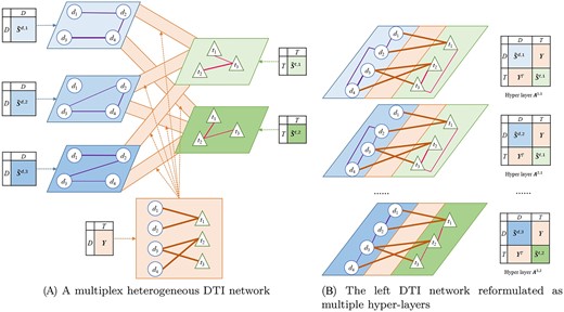
Representing a DTI dataset with three drug and two target similarities as a network. (A) A multiplex heterogeneous network including three drug layers, two target layers and six identical bipartite interaction subnetworks connecting drug and target nodes in each layer. (B) Six multiple hyper-layers, where each of them is composed of a drug and a target layer along with the interaction subnetwork.
The DeepWalk matrix cannot be directly calculated for the complex DTI network that includes two multiplex and a bipartite subnetwork. To facilitate its computation, we consider each combination of a drug and a target layer along with the interaction subnetwork as a hyper-layer, and reformulate the DTI network as a multiplex network containing |$m_d\cdot m_t$| hyper-layers. The hyper-layer incorporating the |$i$|-th drug layer and |$j$|-th target layer is defined by the adjacency matrix
Based on the above reformulation, we compute a DeepWalk matrix |$\boldsymbol{M}^{i,j} \in \mathbb{R}^{(n_d+n_t) \times (n_d+n_t)}$| for each |$\boldsymbol{A}^{i,j}$| using Eq. (3), which reflects node co-occurrences in truncated random walks and captures richer proximity among nodes than the original hyper-layer—especially the proximity between unlinked nodes. In particular, if a pair of unlinked drug and target in |$\boldsymbol{A}^{i,j}$| has a certain level of proximity (non-zero value) in |$\boldsymbol{M}^{i,j}$|, the corresponding relation represented by the DeepWalk matrix could be interpreted as the recovery of their missing interaction, which supplements the incomplete interaction information and reduces the noise in the original dataset. See an example in Supplementary Section A2.1.
However, aggregating all per-layer DeepWalk matrices to the holistic one inevitably leads to substantial loss of layer-specific topology information. To address this limitation, we employ graph regularization for each sparsified drug (target) layer to preserve per layer drug (target) proximity in the embedding space, i.e. similar drugs (targets) in each layer are likely to have similar latent features. To distinguish the utility of each layer, each graph regularization is multiplied by the LIC-based weight of its corresponding layer, which emphasizes the proximity of more reliable similarities. Furthermore, Tikhonov regularization is added to prevent latent features from overfitting the training set.
Optimizing the area under the curve with MDMF
Area under the curve loss functions
AUPR and AUC are two widely used area under the curve metrics in DTI prediction. Modeling differentiable surrogate losses that optimize these two metrics can lead to improvements in predicting performance [10]. Therefore, we instantiate the loss function in Eq. (9) with AUPR and AUC losses, and derive two DeepWalk-based MF models, namely MDMFAUPR and MDMFAUC, that optimize the AUPR and AUC metrics, respectively.
More details for optimizing the AUPR and AUC losses can be found in Supplementary Section A2.4.
Inferring embeddings of new entities
MDMF2A: combining AUPR and AUC
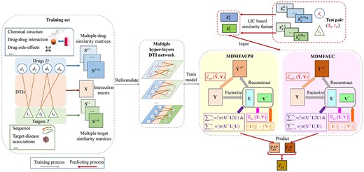
The flowchart of MDMF2A. The DTI dataset, consisting of multiple drug and target similarities, is firstly reformulated as a multiplex DTI network containing multiple hyper-layers. Then, two base models of MDMF2A, namely MDMFAUPR and MDMFAUC, are trained upon the derived multiple hyper-layers DTI network with the instantiation of two area under the curves metric based losses, respectively. Then, given a test pair, its associated similarity vectors are fused according to the LIC-based weights. Next, the two base models leverage these fused similarities to generate the estimation of the test pair, respectively. Lastly, MDMF2A aggregates the outputs of two models using Eq. (18) to obtain its final prediction.
The computational complexity analysis of the proposed methods can be found in Supplementary Section A2.5.
Experimental evaluation and discussion
Experimental Setup
Following [20], four types of cross validation (CV) are conducted to examine the methods in four prediction settings, respectively. In S1, the 10-fold CV on pairs is used, where one fold of pairs is removed for testing. In S2 (S3), the 10-fold CV on drugs (targets) is applied, where one drug (target) fold along with its corresponding rows (columns) in |$\boldsymbol{Y}$| is separated for testing. The 3|$\times $|3-fold block-wise CV, which splits a drug fold and target fold along with the interactions between them for testing, using the interactions between the remaining drugs and targets for training, is applied to S4. AUPR and AUC defined in Eq. (10) and (14) are used as evaluation measures.
To evaluate the performance of MDMF2A in all prediction settings, we have compared it to eight DTI prediction models (WkNNIR [6], NRLMF [7], MSCMF [9], GRGMF [33], MF2A [10], DRLSM [3], DTINet [17], NEDTP [4]) and two network embedding approaches applicable to any domain (NetMF [18] and Multi2Vec [34]). WkNNIR cannot perform predictions in S1, as it is specifically designed to predict interactions involving new drugs or/and targets (S2, S3, S4) [6]. Furthermore, the proposed MDMF2A is also compared with four deep learning-based methods, namely NeoDTI [12], DTIP [5], DCFME [14] and SupDTI [13]. These deep learning competitors can only be applied to the Luo dataset in S1, because they formulate the DTI dataset as a heterogeneous network consisting of four types of nodes (drugs, targets, drug-side effects and diseases) and learn embeddings for all types of nodes. The illustration of all baseline methods can be found in Supplementary Section A3.
The parameters of all baseline methods are set based on the suggestions in the respective articles. For MDMF2A, the trade-off ensemble weight |$\beta $| is chosen from |$\{0,0.01,\ldots ,1.0\}$|. For the two base models of MDMF2A, i.e. MDMFAUPR and MDMFAUC, the number of neighbors is set to |$k=5$|, the window size of the random walk to |$n_w=5$|, the number of negative samples to |$n_s=1$|, the learning rate to |$\theta =0.1$|, candidate decay coefficient set |$\mathcal{C}$|={0.1, 0.2, |$\dotsc $|, 1.0}, the embedding dimension |$r$| is chosen from {50, 100}, |$\lambda _d$|, |$\lambda _t$| and |$\lambda _r$| are chosen from {|$2^{-6}$|, |$2^{-4}$|, |$2^{-2}$|, |$2^{0}$|, |$2^{2}$|}, and |$\lambda _M=0.005$|. The number of bins |$n_b$| in MDMFAUPR is chosen from {11, 16, 21, 26, 31} for small and medium datasets (NR, GPCR and IC), while it is set to 21 for larger datasets (E and Luo). Similar to [3, 7, 9], we obtain the best hyperparameters of our model via grid search, and the detailed settings are listed in Supplementary Table A2.
Results and discussion
Tables 2 and 3 list the results of MDMF2A and its nine competitors on five datasets under four prediction settings. The numbers in the last row denote the average rank across all prediction settings, and ‘*’ indicates that the advantage of DAMF2A over the competitor is statistically significant according to a Wilcoxon signed-rank test with Bergman-Hommel’s correction [35] at 5% level on the results of all prediction settings.
AUPR results in all prediction settings
| Setting | Dataset | WkNNIR | MSCMF | NRMFL | GRGMF | MF2A | DRLSM | DTINet | NEDTP | NetMF | Multi2Vec | MDMF2A |
|---|---|---|---|---|---|---|---|---|---|---|---|---|
| S1 | NR | - | 0.628(6) | 0.64(5) | 0.658(3) | 0.673(2) | 0.642(4) | 0.508(8) | 0.546(7) | 0.455(9) | 0.43(10) | 0.675(1) |
| GPCR | - | 0.844(4.5) | 0.86(3) | 0.844(4.5) | 0.87(2) | 0.835(6) | 0.597(10) | 0.798(8) | 0.831(7) | 0.747(9) | 0.874(1) | |
| IC | - | 0.936(3) | 0.934(4) | 0.913(7) | 0.943(2) | 0.914(6) | 0.693(10) | 0.906(8) | 0.929(5) | 0.867(9) | 0.946(1) | |
| E | - | 0.818(6) | 0.843(3) | 0.832(4) | 0.858(2) | 0.811(7) | 0.305(10) | 0.78(8) | 0.831(5) | 0.736(9) | 0.859(1) | |
| Luo | - | 0.599(6) | 0.603(5) | 0.636(3) | 0.653(2) | 0.598(7) | 0.216(9) | 0.08(10) | 0.615(4) | 0.451(8) | 0.679(1) | |
| |$AveRank$| | - | 5.1 | 4 | 4.3 | 2 | 6 | 9.4 | 8.2 | 6 | 9 | 1 | |
| S2 | NR | 0.562(5) | 0.531(7) | 0.547(6) | 0.564(4) | 0.578(2) | 0.57(3) | 0.339(10) | 0.486(8) | 0.34(9) | 0.338(11) | 0.602(1) |
| GPCR | 0.54(4) | 0.472(7) | 0.508(6) | 0.542(3) | 0.551(2) | 0.532(5) | 0.449(9) | 0.451(8) | 0.356(10) | 0.254(11) | 0.561(1) | |
| IC | 0.491(4) | 0.379(8.5) | 0.479(5) | 0.493(3) | 0.495(2) | 0.466(6) | 0.365(10) | 0.407(7) | 0.379(8.5) | 0.16(11) | 0.502(1) | |
| E | 0.405(4) | 0.288(8) | 0.389(5) | 0.415(3) | 0.422(2) | 0.376(6) | 0.173(10) | 0.33(7) | 0.269(9) | 0.141(11) | 0.428(1) | |
| Luo | 0.485(2) | 0.371(8) | 0.458(6) | 0.462(5) | 0.472(4) | 0.502(1) | 0.187(9) | 0.077(11) | 0.376(7) | 0.079(10) | 0.48(3) | |
| |$AveRank$| | 3.8 | 7.7 | 5.6 | 3.6 | 2.4 | 4.2 | 9.6 | 8.2 | 8.7 | 10.8 | 1.4 | |
| S3 | NR | 0.56(3) | 0.505(7) | 0.519(6) | 0.545(5) | 0.588(1) | 0.546(4) | 0.431(8) | 0.375(9) | 0.359(10) | 0.335(11) | 0.582(2) |
| GPCR | 0.774(3) | 0.69(7) | 0.729(6) | 0.755(5) | 0.787(2) | 0.757(4) | 0.546(10) | 0.684(8) | 0.638(9) | 0.327(11) | 0.788(1) | |
| IC | 0.861(3) | 0.827(7) | 0.838(6) | 0.851(5) | 0.863(2) | 0.855(4) | 0.599(10) | 0.8(8) | 0.791(9) | 0.4(11) | 0.865(1) | |
| E | 0.728(3) | 0.623(8) | 0.711(6) | 0.715(4) | 0.731(2) | 0.712(5) | 0.313(10) | 0.615(9) | 0.656(7) | 0.257(11) | 0.738(1) | |
| Luo | 0.243(5) | 0.08(8) | 0.204(7) | 0.234(6) | 0.292(3) | 0.248(4) | 0.061(9) | 0.046(10) | 0.294(2) | 0.027(11) | 0.299(1) | |
| |$AveRank$| | 3.4 | 7.4 | 6.2 | 5 | 2 | 4.2 | 9.4 | 8.8 | 7.4 | 11 | 1.2 | |
| S4 | NR | 0.309(1) | 0.273(6) | 0.278(5) | 0.308(2) | 0.289(3) | 0.236(8) | 0.249(7) | 0.16(9) | 0.146(11) | 0.149(10) | 0.286(4) |
| GPCR | 0.393(3) | 0.323(6) | 0.331(5) | 0.368(4) | 0.407(1.5) | 0.077(10) | 0.306(7) | 0.29(8) | 0.159(9) | 0.074(11) | 0.407(1.5) | |
| IC | 0.339(4) | 0.194(9) | 0.327(5) | 0.347(3) | 0.352(2) | 0.086(10) | 0.264(6) | 0.251(7) | 0.196(8) | 0.067(11) | 0.356(1) | |
| E | 0.228(3) | 0.074(9) | 0.221(5) | 0.224(4) | 0.235(2) | 0.063(10) | 0.1(7) | 0.112(6) | 0.09(8) | 0.017(11) | 0.239(1) | |
| Luo | 0.132(3) | 0.018(10) | 0.096(6) | 0.106(5) | 0.175(2) | 0.061(7) | 0.035(8) | 0.03(9) | 0.127(4) | 0.002(11) | 0.182(1) | |
| |$AveRank$| | 2.8 | 8 | 5.2 | 3.6 | 2.1 | 9 | 7 | 7.8 | 8 | 10.8 | 1.7 | |
| |$Summary$| | 3.33* | 7.05* | 5.25* | 4.13* | 2.13* | 5.85* | 8.85* | 8.25* | 7.53* | 10.4* | 1.33 | |
AUC results in all prediction settings
| Setting | Dataset | WkNNIR | MSCMF | NRMFL | GRGMF | MF2A | DRLSM | DTINet | NEDTP | NetMF | Multi2Vec | MDMF2A |
|---|---|---|---|---|---|---|---|---|---|---|---|---|
| S1 | NR | - | 0.882(4.5) | 0.882(4.5) | 0.891(2) | 0.884(3) | 0.879(6) | 0.797(9) | 0.846(7) | 0.818(8) | 0.788(10) | 0.892(1) |
| GPCR | - | 0.962(6) | 0.972(4) | 0.978(2) | 0.978(2) | 0.971(5) | 0.916(10) | 0.953(8) | 0.96(7) | 0.93(9) | 0.978(2) | |
| IC | - | 0.982(6) | 0.989(2) | 0.988(4) | 0.989(2) | 0.981(7.5) | 0.938(10) | 0.981(7.5) | 0.985(5) | 0.97(9) | 0.989(2) | |
| E | - | 0.961(8) | 0.981(4) | 0.982(3) | 0.983(2) | 0.964(7) | 0.839(10) | 0.97(5) | 0.966(6) | 0.944(9) | 0.984(1) | |
| Luo | - | 0.922(7) | 0.951(3) | 0.947(4) | 0.966(2) | 0.941(5) | 0.894(9) | 0.929(6) | 0.917(8) | 0.861(10) | 0.97(1) | |
| |$AveRank$| | - | 6.3 | 3.5 | 3 | 2.2 | 6.1 | 9.6 | 6.7 | 6.8 | 9.4 | 1.4 | |
| S2 | NR | 0.825(5.5) | 0.802(7) | 0.826(4) | 0.825(5.5) | 0.833(2) | 0.831(3) | 0.666(11) | 0.786(8) | 0.739(9) | 0.727(10) | 0.837(1) |
| GPCR | 0.914(4) | 0.882(7) | 0.913(5) | 0.924(2.5) | 0.924(2.5) | 0.867(8) | 0.858(9) | 0.885(6) | 0.852(10) | 0.811(11) | 0.925(1) | |
| IC | 0.826(4) | 0.783(9) | 0.825(5) | 0.833(1) | 0.828(2) | 0.796(7) | 0.766(10) | 0.794(8) | 0.803(6) | 0.715(11) | 0.827(3) | |
| E | 0.877(4) | 0.835(7) | 0.858(5) | 0.891(3) | 0.892(2) | 0.799(9) | 0.78(10) | 0.837(6) | 0.811(8) | 0.732(11) | 0.895(1) | |
| Luo | 0.904(5) | 0.897(7) | 0.917(3) | 0.899(6) | 0.927(2) | 0.864(9) | 0.873(8) | 0.907(4) | 0.861(10) | 0.776(11) | 0.937(1) | |
| |$AveRank$| | 4.5 | 7.4 | 4.4 | 3.6 | 2.1 | 7.2 | 9.6 | 6.4 | 8.6 | 10.8 | 1.4 | |
| S3 | NR | 0.82(3) | 0.786(7) | 0.825(2) | 0.845(1) | 0.819(4) | 0.798(6) | 0.756(8) | 0.726(9) | 0.712(10) | 0.703(11) | 0.805(5) |
| GPCR | 0.952(4) | 0.902(9) | 0.946(5) | 0.965(1) | 0.96(3) | 0.917(7) | 0.879(10) | 0.918(6) | 0.909(8) | 0.798(11) | 0.961(2) | |
| IC | 0.958(5) | 0.941(7) | 0.96(4) | 0.965(3) | 0.967(1) | 0.942(6) | 0.907(10) | 0.939(8) | 0.938(9) | 0.866(11) | 0.966(2) | |
| E | 0.935(5) | 0.881(9) | 0.936(4) | 0.943(3) | 0.944(2) | 0.883(8) | 0.841(10) | 0.918(6) | 0.911(7) | 0.815(11) | 0.948(1) | |
| Luo | 0.835(5) | 0.826(9) | 0.828(8) | 0.84(4) | 0.901(2) | 0.801(10) | 0.829(7) | 0.86(3) | 0.831(6) | 0.633(11) | 0.902(1) | |
| |$AveRank$| | 4.4 | 8.2 | 4.6 | 2.4 | 2.4 | 7.4 | 9 | 6.4 | 8 | 11 | 2.2 | |
| S4 | NR | 0.637(5) | 0.597(6) | 0.656(3) | 0.677(1) | 0.649(4) | 0.592(7) | 0.562(8) | 0.548(9) | 0.531(10) | 0.524(11) | 0.661(2) |
| GPCR | 0.871(4) | 0.798(8) | 0.866(5) | 0.89(1) | 0.886(3) | 0.405(11) | 0.803(7) | 0.816(6) | 0.721(9) | 0.581(10) | 0.887(2) | |
| IC | 0.774(5) | 0.658(9) | 0.775(4) | 0.782(2) | 0.776(3) | 0.498(11) | 0.706(6) | 0.702(7) | 0.683(8) | 0.555(10) | 0.783(1) | |
| E | 0.819(3) | 0.695(8) | 0.799(5) | 0.815(4) | 0.821(2) | 0.453(11) | 0.757(6) | 0.744(7) | 0.69(9) | 0.541(10) | 0.827(1) | |
| Luo | 0.819(4) | 0.752(7) | 0.804(5) | 0.745(8) | 0.848(2) | 0.438(11) | 0.787(6) | 0.822(3) | 0.732(9) | 0.513(10) | 0.85(1) | |
| |$AveRank$| | 4.2 | 7.6 | 4.4 | 3.2 | 2.8 | 10.2 | 6.6 | 6.4 | 9 | 10.2 | 1.4 | |
| |$Summary$| | 4.37* | 7.38* | 4.23* | 3.05 | 2.38* | 7.73* | 8.7* | 6.48* | 8.1* | 10.35* | 1.6 | |
The proposed MDMF2A is the best-performing model in most cases for both metrics, achieving the highest average rank in all prediction settings and statistically significantly outperforming all competitors, except for GRGMF in AUC. This demonstrates the effectiveness of our model to sufficiently exploit the topology information embedded in the multiplex heterogeneous DTI network and optimize the two area under the curve metrics. MF2A is the runner-up. Its inferiority to MDMF2A is mainly attributed to the ignorance of high-order proximity captured by random walks and the view-specific information loss caused by aggregating multi-type similarities. GRGMF, WkNNIR, NRMLF, DRLSM and MSCMF come next. They are outperformed by the proposed MDMF2A, because they fail to capture the unique information provided by each view. The two graph embedding based DTI prediction models are usually inferior to other DTI prediction approaches, because they generate embedding in an unsupervised manner without exploiting the interacting information. Specifically, NEDTP using the class imbalance resilient GBDT as the predicting classifier outperforms DTINet which employs simple linear projection to estimate DTIs. Regarding the two general multiplex network embedding methods, NetMF is better than Multi2Vec, because the latter requires dichotomizing the edge weights, which wipes out the different influence of the connected nodes in the similarity subnetwork. In addition, averaging all per-layer embeddings does not distinguish the importance of each hyper-layer, unlike the holistic DeepWalk Matrix used in NetMF, which contributes to the inferiority of Multi2Vec to NetMF as well.
There are some cases where MDMF2A does not achieve the best performance. Some baseline models, such as WkNNIR, NRLMF, GRGMF and MF2A, are better than MDMF2A on NR datasets, implying that the random walk-based embedding generation may not yield enough benefit in the case of small-sized datasets. Besides, concerning the Luo dataset under S2, MDMF2A is outperformed by WKNNIR and DRLSM, which incorporate the neighborhood interaction recovery procedure, in terms of AUPR. In the Luo dataset, the neighbor drugs are more likely to share the same interactions, leading to the effectiveness of neighborhood-based interaction estimation for new drugs. Nevertheless, the AUC results of the two baselines are 3.7% and 8.4% lower than DWFM2A, respectively. Also, MF2A is slightly better than MDMF2A on the IC dataset in terms of AUC under S2 and S3, but the gap of results between them is tiny, e.g. 0.001. Finally, GRGMF achieves better AUC results than MDMF2A on the GPCR dataset under S3 and S4 as well as the IC dataset under S2, mainly because GRGMF learns neighbor information adaptively. But it is worse than MDMF2A in terms of AUPR, which is more informative when evaluating a model under extremely imbalanced class distribution (sparse interaction).
The advantage of MDMF2A is also observed in the comparison with deep learning-based DTI prediction models on the Luo dataset. As shown in Table 4, MDMF2A outperforms all competitors in terms of AUPR, achieving 14% improvements over the best-performing competitor (DCFME). In terms of AUC, MDMF2A is only 1.1% lower than DTIP, and 5.3%, 3.6% and 3.9% higher than NeoDTI, DCFME and SupDTI. Although DTIP emphasizes the AUC performance and slightly outperforms MDMF2A, it suffers a significant decline in the AUPR results. Compared with deep learning competitors, MDMF2A takes full advantage of the information shared by high-order neighbors and explicitly optimizes AUPR and AUC that are more effective than the conventional entropy and focal losses to identifying the less frequent interacting pairs, resulting in better performance.
Results of MDMF2A and Deep Learning models on Luo dataset in S1
| Metric | NeoDTI | DTIP | DCFME | SupDTI | MDMF2A |
|---|---|---|---|---|---|
| AUPR | 0.573(4) | 0.399(5) | 0.596(2) | 0.585(3) | 0.679(1) |
| AUC | 0.921(5) | 0.981(1) | 0.936(3) | 0.933(4) | 0.97(2) |
| Metric | NeoDTI | DTIP | DCFME | SupDTI | MDMF2A |
|---|---|---|---|---|---|
| AUPR | 0.573(4) | 0.399(5) | 0.596(2) | 0.585(3) | 0.679(1) |
| AUC | 0.921(5) | 0.981(1) | 0.936(3) | 0.933(4) | 0.97(2) |
To comprehensively investigate the proposed MDMF2A, we conduct an ablation study to demonstrate the effectiveness of its ensemble framework and all regularization terms and analyze the sensitivity of three important parameters, i.e. |$r$|, |$n_w$| and |$n_s$|. Please see more details in Supplementary Sections A5–A6.
Discovery of novel DTIs
We examine the capability of MDMF2A to find novel DTIs not recorded in the Luo dataset. We do not consider updated golden standard datasets, since they have included all recently validated DTIs collected from up-to-date databases. We split all noninteracting pairs into 10 folds, and obtain predictions of each fold by training an MDMF2A model with all interacting pairs and the other nine folds of noninteracting ones. All noninteracting pairs are ranked based on their predicting scores, and the top 10 pairs are selected as newly discovered DTIs, which are shown in Table 5. To further verify the reliability of these new interaction candidates, we search their supportive evidence from DrugBank (DB) [23] and DrugCentral (DC) [36]. As we can see, 8/10 new interactions (in bold) are confirmed, demonstrating the success of MDMF2A in trustworthy new DTI discovery.
Top 10 new DTIs discovered by MDMF2A from Luo’s datasets
| Drug ID | Drug name | Target ID | Target name | Rank | Database |
|---|---|---|---|---|---|
| DB00829 | Diazepam | P48169 | GABRA4 | 1 | DB |
| DB01215 | Estazolam | P48169 | GABRA4 | 2 | DB |
| DB00580 | Valdecoxib | P23219 | PTGS1 | 3 | - |
| DB01367 | Rasagiline | P21397 | MAOA | 4 | DC |
| DB00333 | Methadone | P41145 | OPRK1 | 5 | DC |
| DB00363 | Clozapine | P21918 | DRD5 | 6 | DC |
| DB06216 | Asenapine | P21918 | DRD5 | 7 | DB |
| DB06800 | Methylnal-trexone | P41143 | OPRD1 | 8 | DC |
| DB00802 | Alfentanil | P41145 | OPRK1 | 9 | - |
| DB00482 | Celecoxib | P23219 | PTGS1 | 10 | DC |
Conclusion
This paper proposed MDMF2A, a random walk and matrix factorization based model, to predict DTIs by effectively mining topology information from the multiplex heterogeneous network involving diverse drug and target similarities. It integrates two base predictors that leverage our designed objective function, encouraging the learned embeddings to preserve holistic network and layer-specific topology structures. The two base models utilize the convex AUPR and AUC losses in their objectives, enabling MDMF2A to simultaneously optimize two crucial metrics in the DTI prediction task. We have conducted extensive experiments on five DTI datasets under various prediction settings. The results affirmed the superiority of the proposed MDMF2A to other competing DTI prediction methods. Furthermore, the practical ability of MDMF2A to discover novel DTIs was supported by the evidence from online biological databases.
In the future, we plan to extend our model to handle attributed DTI networks, including both topological and feature information for drugs and targets.
Incorporating multiple hyper-layers based DeepWalk matrix decomposition and layer-specific graph Laplacian to learn robust node representations that preserve both global and view-specific topology.
MDMF integrates multiplex heterogeneous network representation learning and DTI prediction into a unified optimization framework, learning latent features in a supervised manner and implicitly recoveries possible missing interactions.
MDMF2A, the instantiation of MDMF, optimizes both AUPR and AUC metrics.
Our method statistically significantly outperforms state-of-the-art methods under various prediction settings and can discover new reliable DTIs.
Data and code availability
The source code and data are available could be found at https://github.com/intelligence-csd-auth-gr/DTI_MDMF2A
Funding
This work was supported by the China Scholarship Council (CSC) [201708500095]; the French National Research Agency (ANR) under the JCJC project GraphIA [ANR-20-CE23-0009-01].
Author Biographies
Bin Liu is a lecturer at Key Laboratory of Data Engineering and Visual Computing, Chongqing University of Posts and Telecommunications and received his PhD Degree in computer science from Aristotle University of Thessaloniki. His research interests include multi-label learning and bioinformatics.
Dimitrios Papadopoulos is a PhD student at the School of Informatics, Aristotle University of Thessaloniki. His research interests include supervised machine learning, graph mining, and drug discovery.
Fragkiskos D. Malliaros is an Assistant Professor at Paris-Saclay University, CentraleSupélec and associate researcher at Inria Saclay. His research interests include graph mining, machine learning and graph-based information extraction.
Grigorios Tsoumakas is an Associate Professor at the Aristotle University of Thessaloniki. His research interests include machine learning (ensembles, multi-target prediction) and natural language processing (semantic indexing, keyphrase extraction, summarization)
Apostolos N. Papadopoulos is Associate Professor at the School of Informatics, Aristotle University of Thessaloniki. His research interests include data management, data mining and big data analytics.
References
