


Abstract
Anatomical Therapeutic Chemical (ATC) classification for compounds/drugs plays an important role in drug development and basic research. However, previous methods depend on interactions extracted from STITCH dataset which may make it depend on lab experiments. We present a pilot study to explore the possibility of conducting the ATC prediction solely based on the molecular structures. The motivation is to eliminate the reliance on the costly lab experiments so that the characteristics of a drug can be pre-assessed for better decision-making and effort-saving before the actual development. To this end, we construct a new benchmark consisting of 4545 compounds which is with larger scale than the one used in previous study. A light-weight prediction model is proposed. The model is with better explainability in the sense that it is consists of a straightforward tokenization that extracts and embeds statistically and physicochemically meaningful tokens, and a deep network backed by a set of pyramid kernels to capture multi-resolution chemical structural characteristics. Its efficacy has been validated in the experiments where it outperforms the state-of-the-art methods by 15.53% in accuracy and by 69.66% in terms of efficiency. We make the benchmark dataset, source code and web server open to ease the reproduction of this study.
Introduction
To identify a given compound into Anatomical Therapeutic Chemical (ATC) system for studying its possible active ingredients, as well as its therapeutic, pharmacological and chemical properties, is of great significance to both drug development and basic research. A commonly adopted ATC system (https://www.whocc.no/atc/structure_and_principles/) is the one developed by the World Health Organization (WHO). It is a hierarchical classification system that contains five levels of categories, in which the first level consisting of 14 groups (as shown in Table 1) has been widely employed to develop methods for ATC classification in the recent decade.
Comparison of the two benchmark datasets over the level-1 ATC codes.
| ATC-SMILES | Chen-2012 [4] | Overlapped | ||
|---|---|---|---|---|
| Code | Anatomical/Pharmacological Group | (#drugs) | (#drugs) | (#drugs) |
| A | Alimentary tract and metabolism | 618 | 540 | 517 |
| B | Blood and blood-forming organs | 158 | 133 | 126 |
| C | Cardiovascular system | 625 | 591 | 581 |
| D | Dermatologicals | 455 | 421 | 402 |
| G | Genito urinary system and sex hormones | 285 | 248 | 245 |
| H | Systemic hormonal preparations, excl. sex hormones and insulins | 143 | 126 | 123 |
| J | Antiinfectives for systemic use | 621 | 521 | 501 |
| L | Antineoplastic and immunomodulating agents | 402 | 232 | 223 |
| M | Musculo-skeletal system | 227 | 208 | 204 |
| N | Nervous system | 826 | 737 | 724 |
| P | Antiparasitic products, insecticides and repellents | 138 | 127 | 122 |
| R | Respiratory system | 462 | 427 | 419 |
| S | Sensory organs | 415 | 390 | 376 |
| V | Various | 252 | 211 | 204 |
| Total #drugs (counted by virtual drugs defined in [4]) | 5627 | 4912 | 4767 | |
| Total #drugs (counted by the number of identical SMILES sequences) | 4545 | 3883 | 3785 | |
ATC classification is modeled as a multi-label classification problem, where a given compound is assigned to one or several labels indicating its belongingness to the 14 groups. The study dates back to 2008 when Dunkel et al. [1] proposed the first method that predicts a single label of a compound using its physicochemical properties and molecular fingerprints. A great effort from researchers has been made since then by extending the problem from the single-label prediction [1–3] to multi-label prediction [4–18], introducing unified benchmark ATC datasets and evaluation methodology [4, 19], enriching the features with additional information such as chemical–chemical interactions [4–11, 13–18, 20, 21], structural similarities [2, 4–7, 9–11, 13–18, 20, 21] and chemical ontology [6, 9, 14, 20], and increasing the availability with web servers [1, 3, 5, 6, 12, 13].
In Figure 1, we summarize 18 representative works proposed in recent 10 years to study the evolution. Two trends can be observed. One is the introduction of deep learning (DL) (e.g. GCN in [15], CNN in [14, 15]) to take the place of traditional machine learning methods (e.g. SVM in [2, 20], ML-GKR in [5, 6]). This is not surprising because DL is considered as a game changer in a wide range of disciplinary for its power of modeling complex relations. The other trend is the integration of more and more data sources for richer representations. For example, the compound descriptions from Wikipedia are used to construct the word embedding in [15], and the chemical subgraph similarities are employed in [5, 9, 13, 15, 16]. The inclusion of new resources can enrich the representations but may introduce additional issues at the same time. For example, it increases the complexity of the representations and models, which requires additional computing power for reproduction and deployment, not to mention the fact that some methods even require additional efforts to query external tools like Rdkit [22] or web services like SIMCOMP (https://www.genome.jp/tools/simcomp/) and SUBCOMP (https://www.genome.jp/tools/subcomp/). More importantly, most of these new resources are interactions extracted from STITCH [23] which is a dataset collected from previous clinical trials, physicochemical experiments and meta analysis. The reliance on STITCH makes the ATC prediction depend on lab experiments and thus less feasible and practical for new/unseen drugs/compounds.
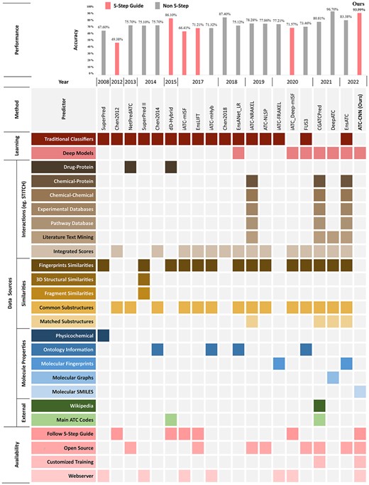
Summary of ATC classification methods in the last 10 years.
In this paper, we present a pilot study to explore the feasibility of conducting ATC classification with a single resource, which simplifies both the data acquisition process and the model complexity. More specifically, we generate the representations based only on molecular structures. We argue that the (conventional) structural models such as molecular fingerprints and graphs are incomplete and suffer from information loss. For example, the molecular fingerprints are generated by simplifying the structure into binary vectors (e.g. Morgan fingerprint [24], MACCSKeys [25]). The molecular graphs are generated by transforming the structures into low-dimensional manifolds in which only the neighboring information to adjacent atoms are preserved [16]. The high-order or continuous information like the functional groups or branches are either simplified or ignored in these models. Therefore, a majority of previous methods are using these structural information as a supplementary source to the trail-dependent sources (e.g. STITCH [23]). In this paper, we propose to model the structure directly to avoid information loss. Specifically, we use the Simplified Molecular Input Line Entry System (SMILES) [26] as the data source, and leverage the power of deep learning to model the complex relations behind. More importantly, SMILES is used as the sole data source so that the reliance on lab experiments is eliminated in this study. We demonstrate that this can achieve comparable (or even superior) performance to those of the state-of-the-art ATC prediction methods which are using multiple data sources. The structure-only nature gives the proposed method the potential to save a significant amount of expensive resources for drug development or basic research (at least for that of pre-research steps). Other contributions of this study include: (1) we collect a new ATC dataset of 4545 compounds/drugs, which can be used either to develop the structure-only methods in the future, or as the supplementary to existing benchmarks; (2) the dataset, source code and web server will be publicly available; and (3) we propose a light-weight DL model called ATC-CNN which outperforms the state-of-the-art methods significantly in terms of both effectiveness and efficiency. The representations are straightforward and with better explainability.
This paper is organized following the five-step guideline in [27] which is widely adopted in ATC studies [4, 5, 7, 13, 20] as (1) benchmark dataset, (2) sample formulation, (3) operation algorithm, (4) anticipated accuracy and (5) web-server.
Materials and Methods
Benchmark Dataset
We construct a new benchmark ATC-SMILES for ATC classification in this study. ATC-SMILES consists of 4545 compounds/drugs and their SMILES sequences. The benchmark is with the maximum coverage (81.34%) of KEGG dataset [28] which contains all 5588 known drugs/compounds used for ATC analysis. Prior to this benchmark, the most widely adopted one is Chen-2012 [4] which covers 3883 (69.49%) drugs in KEGG and is mainly used for generating inter-drug correlations (e.g. STITCH [23]). The two benchmarks are compared in Table 1. ATC-SMILES is designed to be inclusive to Chen-2012, but there are 2.16% misalignment due to the mismatching of drug IDs that we will explain soon. ATC-SMILES can be extended with new drugs much easier than previous benchmarks as long as the SMILES sequences are available. Trails/experiments are not a must.
The process for generating ATC-SMILES starts by collecting all the 5588 drug IDs from KEGG using BioPython [29]. With the IDs as primary keys, we search the CIDs over PubChem dataset [30] for SMILES representations of these drugs. We skip drugs when there are no matched items or corresponding SMILES representations in PubChem (e.g. KEGG D11856: Empagliflozin, linagliptin and metformin hydrochloride). This results in the exclusion of 712 drugs.
Note that we generate the class labels using the same merging process that has been adopted in previous studies. The process merges two ATC codes as a single label if they are the same at level-1, otherwise, considers them as two separated labels. For example, Ketoprofen is with two ATC codes M01AE03 and M02AA10, but its level-1 code is consistent as M (i.e. MUSCULO-SKELETAL SYSTEM). Therefore, Ketoprofen is assigned with a single label M. Ciprofloxacin is with four ATC codes J01MA02, S01AE03, S02AA15 and S03AA07. It is assigned with two labels of J (from J01MA02 for ANTIINFECTIVES FOR SYSTEMIC USE) and S (by combining S01AE03, S02AA15 and S03AA07 for SENSORY ORGANS).
Problem Formulation
In the proposed method, we learn the representations |$\textbf{x}$| using SMILES embedding and implement the |$f$| using a light-weight convolutional network (CNN) with parameters |$ {\theta }$|. Binary Cross Entropy is adopted as the loss |$L(\hat{\textbf{y}},\textbf{y})$|. Let us breakdown our introduction into these components.


Tokenization and Representation Generation
We generate the representation |$\textbf{x}$| of a drug/compound using its SMILES sequence. The first step is to split a sequence into a set of tokens. Although the idea is intuitive, there are only a few works in literature which have studied this problem. In [31], Goh et al. propose SMILES2vec in which every character in the SMILES sequence is considered as a token for embedding, while in [32], Zhang et al. propose SPVec which breaks a sequence into tokens using a sliding window of size 3. Tokens generated with those methods may not be physicochemically meaningful, and less representative when used for embedding. We address this issue with an interactive process between a statistical tokenizer and human experts.
The motivation is to find tokens that are both statistically meaningful so as to make the modeling effective and efficient, and physicochemically meaningful to human experts so as to increase the explainability of the method. As shown Figure 2, the proposed tokenization process consists of three parts: (1) a Token Extractor to propose candidate tokens and corresponding confidence scores; (2) a Domain Knowledge Injector in which human experts identify physicochemically meaningful tokens from the highly confident candidates so as to construct a token dictionary as well as generalize rules for further extraction; and (3) a Sequence Validator which finds the best partition among all combinations of tokens for a given sequence.
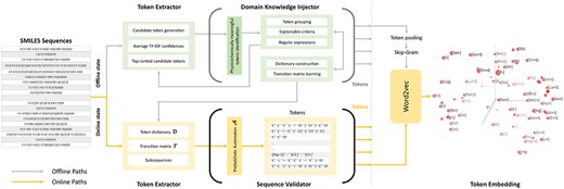
Token Generation and Embedding. A dictionary consisting of the best set of tokens is learned jointly by the statistical extractor and human experts (offline), and used to conduct the tokenization (online). The token embeddings are learned by retraining the Word2vec in an ATC setting.
Token Extractor
The Token Extractor has offline and online states. The offline state is for learning the token dictionary |$\mathcal{D}$| by working with the domain knowledge injector, while the online state is for extracting tokens for ATC classifications by working the Sequence Validator. We will introduce the offline state and delay the introduction of online state until that of the validator.
Human Knowledge Injector
The Injector takes the top-|$20$| candidates as the input and involves human experts in the learning. The human experts identify the physicochemically meaningful tokens from the candidates and add them into the token dictionary |$\mathcal{D}$|. In addition, the experts conduct two generalization steps to inject knowledge into the extractor and validator, respectively.
One is to categorize the tokens in the dictionary into a set of groups |$\{g_i\}$| according to their physicochemically characteristics. For each group, the experts generate selection criteria to make the results explainable (as the results shown in Figure 2). A set of regular expressions is also generated for each group by observing the token patterns. The token extractor will use these expressions for more efficient extraction. This makes the results generalizable. For example, a regular expression ‘[??+?]’ generated from tokens ‘[Fe+4]’ can help identify ‘[Lu+3]’, ‘[Cu+2]’ and ‘[Al+3]’ in the future. The dictionary learning process jointly conducted by the extractor and injector is then repeated until no tokens can be identified and the dictionary |$\mathcal{D}$| is ready. This results in eight groups of 109 tokens as shown in Figure 3.
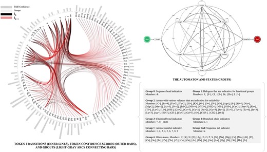
Tokens, Transitions, Groups and the Probabilistic Automaton.
Sequence Validator
Generating the Representation |$\textbf{x}$| using Word Embedding
Once the tokens are extracted from sequences, we pool them for word embedding. It generates for each token a vector representation |$\textbf{t}\in \mathbb{R}^m$|, so that the representation can be used to generate the drug/compound representation |$\textbf{x}\in \mathbb{R}^d$|. To this end, word embedding learns a linear space |$\mathbb{R}^m$|, in which tokens, once being represented into the space, distribute closely with their contextually related tokens (i.e. those co-occur frequently within the same sliding windows with them) while far from the non-related ones. For example, the distance of representations of ‘C’ and ‘O’ is smaller than that of the ‘[Cl-]’ and ‘=’.
We adopt the Word2Vec [36] and Skip-gram model [37] to conduct the learning by setting the dimensionality of the target space |$m=300$|, the context window size of 12 and the negative sample rate at 15. In this case, Skip-gram generates positive training examples by taking each token in a 15-token window as the predictor, the rest of 14 tokens as the context target and a label |$1$| indicating the contextual relatedness. By contrast, Skip-gram generates negative training example by replacing the context targets with those from different windows (randomly selected) and setting the label to |$0$| indicating the non-contextual relatedness.
Model |$f$| and Parameters |$\boldsymbol{\theta }$|
We design the model |$f$| with an ad hoc CNN by following the practice of TextCNN [38] family which is recognized with promising performance on text liked sequences. To ease the description, we call it ATC-CNN hereafter. As shown in Figure 4, ATC-CNN is a seven-stream and light-weight CNN. The seven streams take the |$\textbf{x}\in \mathbb{R}^{787\times 300}$| as the input and process it in parallel, which results in seven feature maps. The feature maps are then flattened and concatenated as a single feature vector for the inference in the fully connected (FC) layers.

Representation generation using ATC-CNN and the receptive fields captured for Aceclofenac. The kernel pyramid enables a multi-resolution modeling and embedding of compound structures. It captures a double-bond and an Oxygen atom at the kernel size 2, expands to a Carbanyl group at size 4 and includes a functional group of Esters at size 6. More branches and groups are included and jointly embedded while the kernel is expanding to size 24.
Convolutional Layers
The convolution kernel |$\boldsymbol{\kappa }_i^c$| of the |$c^{th}$| channel of the |$i^{th}$| stream is with a size of |$787\times 2m_i$|, which constraints the convolution to be conducted only along the first dimension of |$\textbf{x}$| (i.e. the kernel moves across tokens). This makes the convolution work as a local structure extractor to summarize the relation of the |$2m_i$| adjacent tokens.
FC Layers and Predictions |$\hat{\textbf{y}}$|
Loss Function |$L(\hat{\textbf{y}},\textbf{y})$| and Parameter Learning
Results and Discussion
Metrics for Multi-label ATC Classification
Cross-validation
We use jackknife test[47] for cross-validation, which is considered the least arbitrary method that outputs unique outcome for the ATC benchmark dataset [48]. Therefore, jackknife test is commonly adopted for evaluating the ATC predictors in almost all the previous studies [4–7, 9–15].
Comparison with SOTA Methods
We compare the performance of the proposed ATC-CNN with |$14$| SOTA methods that are with performance reported in the five metrics. The 14 methods include those using various representations (chemical interactions, chemical structural features, molecular fingerprint features, pre-trained word embedding, ATC codes association information and drug ontology information) and models (SVM, ML-GKR, LIFT, NLSP, RAKEL, RR, CNN, GCN, hMuLab and LSTM). It is the most comprehensive comparison that we can find in literature. To be consistent with previous studies, we have also conducted experiments on the Chen-2012 benchmark. However, due to the aforementioned missing SIMILES issue, we have to set the representations of the 98 out of 3883 drugs with absent SIMILES structures (|$2.52\%$| of the dataset) to zero vectors. The results are shown in Table 2.
Performance comparison with SOTA methods. The best results are in bold font.
| Method | Year | Dataset | #Drugs | Rep. | Model | Aiming | Coverage | Accuracy | Absolute | Absolute | |||
|---|---|---|---|---|---|---|---|---|---|---|---|---|---|
| |$\uparrow $| | |$\uparrow $| | |$\uparrow $| | True |$\uparrow $| | False |$\downarrow $| | |||||||||
| Chen et al. [4] | 2012 | Chen-2012 | 3883 | I | S | Similarity Search | 50.76% | 75.79% | 49.38% | 13.83% | 8.83% | ||
| iATC-mISF[5] | 2017 | Chen-2012 | 3883 | I | S | F | ML-GKR | 67.83% | 67.10% | 66.41% | 60.98% | 5.85% | |
| iATC-mHyb[6] | 2017 | Chen-2012 | 3883 | I | S | F | O | ML-GKR | 71.91% | 71.46% | 71.32% | 66.75% | 2.43% |
| EnsLIFT[7] | 2017 | Chen-2012 | 3883 | I | S | F | LIFT | 78.18% | 75.77% | 71.21% | 63.30% | 2.85% | |
| EnsANet_LR[9] | 2018 | Chen-2012 | 3883 | I | S | F | CNN,LIFT,RR | 75.40% | 82.49% | 75.12% | 66.68% | 2.62% | |
| EnsANet_LR|$\otimes $|DO[9] | 2018 | Chen-2012 | 3883 | I | S | F | O | CNN,LIFT,RR | 79.57% | 83.35% | 77.78% | 70.90% | 2.40% |
| ATC-NLSP[10] | 2019 | Chen-2012 | 3883 | I | S | F | NLSP | 81.35% | 79.50% | 78.28% | 74.97% | 3.43% | |
| iATC-NRAKEL[11] | 2020 | Chen-2012 | 3883 | I | S | RAKEL,SVM | 78.88% | 79.36% | 77.86% | 75.93% | 3.63% | ||
| iATC-FRAKEL[12] | 2020 | Chen-2012 | 3883 | F | RAKEL,SVM | 78.51% | 78.40% | 77.21% | 75.11% | 3.70% | |||
| FUS3[14] | 2020 | Chen-2012 | 3883 | I | S | F | CNN,LSTM,LIFT,RR | 87.55% | 69.73% | 73.46% | 68.71% | 2.38% | |
| FUS3|$\otimes $|DO[14] | 2020 | Chen-2012 | 3883 | I | S | F | O | CNN,LSTM,LIFT,RR | 79.79% | 84.22% | 79.64% | 73.04% | 2.09% |
| iATC_Deep-mISF[13] | 2020 | Chen-2012 | 3883 | I | S | F | O | DNN | 74.70% | 73.91% | 71.57% | 67.01% | 0.00% |
| CGATCPred[15] | 2021 | Chen-2012 | 3883 | I | S | E | A | CNN,GCN | 81.94% | 82.88% | 80.81% | 76.58% | 2.75% |
| EnsATC[18] | 2022 | Chen-2012 | 3883 | I | S | F | hMuLab,LSTM | 91.39% | 84.32% | 83.38% | 80.09% | 1.31% | |
| ATC-CNN | 2022 | Chen-2012 | 3883 | S | CNN | 93.01% | 90.72% | 90.53% | 87.77% | 1.53% | |||
| ATC-CNN | 2022 | ATC-SMILES | 4545 | S | CNN | 95.83% | 94.14% | 93.99% | 91.77% | 0.94% | |||
Representation (Rep.) abbreviations: I - Chemical interactions, S - Chemical structural features, F - Molecular fingerprint features, O - Drug ontology information, E - Pre-trained word embedding, and A - ATC codes association information.
ATC-CNN outperforms the SOTA methods by |$1.62\%$|, |$6.40\%$|, |$7.15\%$|, |$7.68\%$| and |$0.22\%$| on Chen-2012[4] in Aiming, Coverage, Accuracy, Absolute True and Absolute False, respectively. The superiority of the proposed method is more obvious on Absolute True, and Absolute False, which are two of the strictest metrics. This is an indication that ATC-CNN is better in providing the exactly matched labels to these of the ground-truth (measured by Absolute True), and is less possible to make all labels wrong (measured by Absolute False). It is a preferable characteristic in drug development because the risk-benefit ratio of developing a new drug can be better evaluated before starting the costly experimental process.
Comparison on Aligned Dataset
Although ATC-SMILES is with a larger scale than that of Chen-2012[4], there are some mis-aligned items. We remove these items to generate a subset consisting of 3785 drugs/compounds which are shared in common by the ATC-SMILES and Chen-2012. We call this set ATC-SMILES-Aligned hereafter. With ATC-SMILES-Aligned, we can study the characteristics of ATC-CNN in more detail by comparing its performance with that of CGATCPred[15]. CGATCPred is the only one in literature that has source code available and allows users to retrain the model by themselves (see statistics in Figure 1).
Overall Performance: As shown in Table 3, ATC-CNN outperforms the CGATCPred by 16.63%, 12.73%, 15.53%, 16.91% and 1.84% in Aiming, Coverage, Accuracy, Absolute True and Absolute False, respectively. Given the fact that the number of parameters of ATC-CNN (|$5.44\ million$|) is 97.43% less than that of CGATCPred (|$211.98\ million$|), this is a surprising result. Further benefiting from the light-weight model, ATC-CNN is 229.55% and 107.89% faster than CGATCPred in training and testing, respectively.
Performance comparison on ATC-SMILES-Aligned.
| Predictor | Effectiveness | Efficiency | |||||||
|---|---|---|---|---|---|---|---|---|---|
| Model | #parameters | Aiming | Coverage | Accuracy | Absolute | Absolute | Training |$\downarrow $| | Training |$\downarrow $| | Testing |$\downarrow $| |
| (million) | |$\uparrow $| | |$\uparrow $| | |$\uparrow $| | True |$\uparrow $| | False |$\downarrow $| | (ms./epoch) | (ms./sample) | (ms./sample) | |
| CGATCPred[15] | 211.98 | 78.18% | 79.91% | 76.92% | 72.84% | 3.04% | 67036.75 | 16.84 | 3.95 |
| ATC-CNN | 5.44 | 94.81% | 92.64% | 92.45% | 89.75% | 1.20% | 19284.53 | 5.11 | 1.90 |
Class-dependent Performance: To investigate the generalizability of the proposed method, we compare the performance of the two methods over labels/classes. The results are shown in Figure 5.
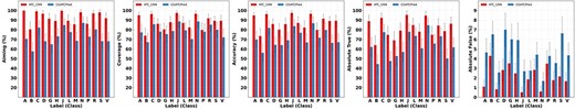
Performance comparison over labels/classes. ATC-CNN outperforms CGATCPred and is with smaller standard deviation.
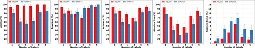
Performance comparison over number of labels/classes. ATC-CNN outperforms CGATCPred and is with smaller standard deviation.
The superiority of the proposed method is observed over all classes. For example, ATC-CNN obtains an accuracy above 80% on 13 out of the 14 labels/classes, while there are only four classes on which CGATCPred demonstrates a comparable performance. Furthermore, ATC-CNN appears more stable than CGATCPred, indicated by its smaller standard deviation than that of CGATCPred.
It is worth mentioning that both methods show inferior performance on class B with the accuracy below 80%. This is due to fact that class B is with the largest portion of inorganic salt (23.81%) when compared with that of other classes (less than 1%). Inorganic salt (e.g. MgCl2, NaCl, KCl, CaCl2) are with a SMILES length ranging from 3 to 7, which is much shorter than the standard representation length 787. This introduces an overwhelming number of zeros into their representations (because of the padding) which makes them less informative than others.
In addition, the most significant performance difference of the two methods is observed in class A, where ATC-CNN outperforms CGATCPred by 25.03%. The reason is that class A contains 28.85% of multi-label instances of ATC-SMILES-Aligned. As we will see in the next section that the majority of performance gain of ATC-CNN over CGATCPred is obtained on multi-label instances, it is not surprising that the performance difference on class A is also unique among the 14 classes.
Performance over #Labels: We also compare the performance over the number of labels. ATC-CNN outperforms CGATCPred significantly as expected. However, on the metric Coverage, ATC-CNN shows inferior performance over CGATCPred. The reason is that CGATCPred is a method with preference on the recall. It tends to output more labels and puts less focus on the precision. When investigating jointly with the metrics of Aiming and Accuracy, it is more evident that ATC-CNN obtains a better balance between the precision and recall.
Both methods obtain a U-shape performance when the number of labels increases. This is counterintuitive, because drugs with more labels (ATC codes) usually raise more challenges to the models than those with less. The proposed method makes correct predictions for drugs with six labels (and ATC codes up to 11) such as Chlorhexidine Gluconate (five labels or eight codes), Prednisolone sodium phosphate (6 labels or 10 codes) and Dexamethasone acetate (6 labels or 11 codes). The performance drops down to the valley at point 3 and climbs up afterwards. This can be explained by a Bernoulli process in which the network outputs six binary variables corresponding to the six labels/classes, and the variables are independent of each other. It becomes intuitive instantly that the maximum entropy obtains when three out of the six variables are with values of 1, while the rest of others are all 0.
In terms of single (|$\#labels=1$|) versus multiple (|$\#labels>1$|) labels, the performance gain of ATC-CNN over CGATCPred on multi-label ones is more significant than on single-label instances with 35.47%, 2.49%, 22.29%, 27.61% and 4.55% in Aiming, Coverage, Accuracy, Absolute True and Absolute False, respectively.
Web Server
In addition to making the source code of ATC-CNN open on Github.com, we develop a web server at http://www.aimars.net:8090/ATC_SMILES/ to increase the availability of the method and dataset. The web server takes a drug/compound ID, or SMILES sequence as the input, and predicts the labels and top-five related drugs/compounds. The ID and sequence are not necessarily from ATC-SMILES, the server is capable of predicting labels for any drugs or compounds with valid IDs or sequences.
Conclusion
We present a pilot study to explore the possibility of conducting ATC classification solely based on the structural information (i.e. SMILES sequences). A new dataset, which is with larger scale than the traditional one, is constructed for the study. We also propose a light-weight and ad hoc framework for ATC classification. The framework is with better explainability than previous methods because it extracts and embeds tokens that are both statistical and physicochemically meaningful, and generates compound representations by capturing the multi-resolution structural characteristics. Its efficacy has been validated in the experiments. This indicates that the ATC codes of drug/compound can be predicted prior to the costly biochemical trails/experiments to save the effort of drug development or basic research.
Construct a new benchmark ATC-SMILES for ATC classification which is with larger scale than transitional benchmarks and eliminates the reliance on STITCH database.
Propose a new tokenization process which extracts and embeds statistically and physicochemically meaningful tokens.
Propose a molecular structure-only deep learning method which is with better explainability.
The proposed method outperforms the state-of-the-art methods.
Code and data availability
The dataset, source code, and web server are open to public at https://github.com/lookwei/ATC_CNN for easier production of this study.
Funding
This work was supported by the National Natural Science Foundation of China under Grant 61872256 and in part by the Internal Research Fund from the Hong Kong Polytechnic University (No. P0036200).
Author Biographies
Yi Cao is a postgraduate student with the Dept. of Computer Science, Sichuan University, China. His research interests include drug representation learning and drug properties predication.
Zhen-Qun Yang is a project fellow with the Dept. of Computing, Hong Kong Polytechnic University, Kowloon, Hong Kong. She was a postdoctoral fellow with the Dept. of Biomedical Engineering, Chinese University of Hong Kong, Kowloon, Hong Kong when the study was initiated. Her research interests include health computing, multimedia retrieval, image processing, and machine learning.
Xu-Lu Zhang is a Ph.D student with the Dept. of Computing, Hong Kong Polytechnic University, Kowloon, Hong Kong. He was a postgraduate student with the Dept. of Computer Science, Sichuan University, China, when the study was initiated. He works on interpretable deep learning and biological signal processing.
Wenqi Fan is a research assistant professor with the Dept. of Computing, Kowloon, Hong Kong Polytechnic University. His research interests are in the broad areas of machine learning and data mining, with a particular focus on Recommender Systems, Graph Neural Networks, and Trustworthy AI.
Yaowei Wang is a tenured associate professor with Peng Cheng Laboratory, Shenzhen, China. His research interests include machine learning, multimedia content analysis, and understanding. He was the recipient of the second prize of the National Technology Invention in 2017 and the first prize of the CIE Technology Invention in 2015.
Jiajun Shen obtained his PhD. in Computer Science from the University of Chicago in 2018. Currently he holds the position of Chief AI Scientist at TCL Research and research associate at the University of Hong Kong. His research focuses on large scale representation learning and neural machine translation.
Dong-Qing Wei is a full professor at the School of Life Sciences and Biotechnology, Shanghai Jiao Tong University. He made many groundbreaking contributions to the development of bioinformatics techniques and their interdisciplinary applications to systems of ever-increasing complexity.
Qing Li is a chair professor with and the department head of the Department of Computing, Hong Kong Polytechnic University, Hong Kong. His current research interests include multimodal data management, conceptual data modeling, social media, Web services, and e-learning systems.
Xiao-Yong Wei is a professor with and the head of the Dept. of Computer Science, Sichuan University of China, and a visiting professor of the Dept. of Computing, Hong Kong Polytechnic University. Kowloon, Hong Kong. His research interests include multimedia computing, health computing, computer vision, and machine learning.
References
Author notes
Yi Cao and Zhen-Qun Yang contributed equally to this work and share first authorship.
