


Abstract
Many DNA methylation (DNAm) data are from tissues composed of various cell types, and hence cell deconvolution methods are needed to infer their cell compositions accurately. However, a bottleneck for DNAm data is the lack of cell-type-specific DNAm references. On the other hand, scRNA-seq data are being accumulated rapidly with various cell-type transcriptomic signatures characterized, and also, many paired bulk RNA-DNAm data are publicly available currently. Hence, we developed the R package scDeconv to use these resources to solve the reference deficiency problem of DNAm data and deconvolve them from scRNA-seq data in a trans-omics manner. It assumes that paired samples have similar cell compositions. So the cell content information deconvolved from the scRNA-seq and paired RNA data can be transferred to the paired DNAm samples. Then an ensemble model is trained to fit these cell contents with DNAm features and adjust the paired RNA deconvolution in a co-training manner. Finally, the model can be used on other bulk DNAm data to predict their relative cell-type abundances. The effectiveness of this method is proved by its accurate deconvolution on the three testing datasets here, and if given an appropriate paired dataset, scDeconv can also deconvolve other omics, such as ATAC-seq data. Furthermore, the package also contains other functions, such as identifying cell-type-specific inter-group differential features from bulk DNAm data. scDeconv is available at: https://github.com/yuabrahamliu/scDeconv.
Introduction
Many diseases show alterations in RNA expression and DNA methylation (DNAm) [1–3]. However, their interpretation is hampered by cell-type heterogeneity of the samples because the overall signatures captured by bulk RNA or DNAm technologies only measure the average behavior [4–9]. So the changes in gene expression or DNAm may only reflect cell-type composition changes rather than cell states changes. Hence, computational methods have been developed to infer cell-type proportions from bulk data [5]. These methods, known as deconvolution methods, provide a means to distinguishing between changes in cell-type composition and cell state.
Almost all these methods require a priori knowledge, such as the cell-type-specific gene expression or DNAm signature reference [10, 11], obtained from the bulk RNA or DNAm profiling of purified cell types. In addition, single-cell RNA sequencing (scRNA-seq) technologies have provided an approach to characterizing cell-type transcriptomic signatures on a single-cell level [12].
Based on these resources, different deconvolution methods use different frameworks to estimate cell-type composition. CIBERSORTx uses support vector regression to deconvolve cell proportions [13, 14]; TIMER quantifies immune cell infiltration with specific features of cancer samples considered [15]; DWLS applies a weighted least square approach to conduct deconvolution [16].
Meanwhile, the accumulation of scRNA-seq data essentially promotes the application of these tools. Hence, cell deconvolution becomes promising for bulk RNA data. However, for bulk DNAm data, the application of these methods is limited because they are single-omics methods and can be used on bulk DNAm data only if a DNAm reference is available. They do not utilize the scRNA-seq resource efficiently this time. Hence, a multi-omics method to deconvolve bulk DNAm data via the scRNA-seq resource becomes essential to overcome the problem that single-cell DNAm data are rare. This is the motivation for developing the R package scDeconv here, which performs cell deconvolution not only in a single-omics manner but also in a multi-omics manner.
During the preparation of this work, a method named EpiSCORE was published, which proposes to impute a DNAm reference from an scRNA-seq signature, depending on the DNAm-gene expression relationship, and then use it to deconvolve bulk DNAm data [17]. This promotes cell deconvolution for bulk DNAm data. However, because it infers DNAm reference from the DNAm-RNA relationship, its logical axis is RNA imputable DNAm -> cell composition, rather than that of the usual case, which is just DNAm -> cell composition. This shrinkage discards much information from the DNAm sites without a clear relationship to RNA level but still associated with cell composition. In addition, because its DNAm imputation models are trained from two public datasets in advance and then applied generally on all the tissues to be deconvolved, some tissue-specific information can be missed.
On the other hand, the R package scDeconv uses a different strategy to perform the multi-omics deconvolution. Because many paired RNA-DNAm data, such as the ones in The Cancer Genome Atlas (TCGA), are available currently, this package utilizes this resource. It assumes that paired samples have similar cell compositions. So the cell content information deconvolved from the scRNA-seq and paired RNA data can be transferred to the paired DNAm samples. Then several LASSO models are trained to predict these cell contents with DNAm features and also adjust the paired RNA deconvolution in a co-training manner. Finally, the LASSO models are ensembled together to predict the cell compositions (relative cell-type abundances, the same with the remaining parts of this manuscript). When used on the testing datasets, this method performs better than EpiSCORE because it leverages more information by including the matched RNA-DNAm data.
Methods and results
Package overview
The package has three modules (Figure 1). The first is a single-omics deconvolution module. Its function scRef can construct cell transcriptomic references from scRNA-seq data (see Supplementary Data, Figure S1). Next, the reference is transferred to the function refDeconv. It performs a recursion process to solve a constrained linear model to deconvolve bulk RNA data with the reference. In addition, our package scDeconv contains a function also named scDeconv. It is the wrapper of scRef and refDeconv so that the reference construction and cell deconvolution steps can be completed with one function. Their details are in Supplementary Data.
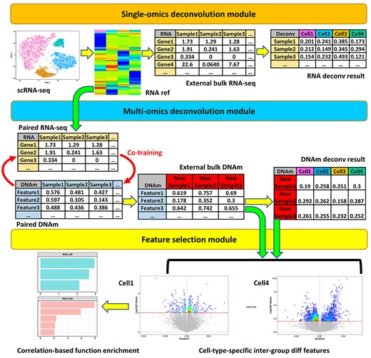
Package modules. The package has three modules: the single-omics deconvolution module, the multi-omics deconvolution module and the feature selection module.
The second module is a multi-omics deconvolution module (see Supplementary Data, Figure S2). Its function epDeconv deconvolves bulk DNAm microarray data via an RNA reference. It also needs another dataset with paired RNA-DNAm data. Because of the pairing, we assume the cell contents of the RNA and DNAm samples are similar. Hence, the deconvolution results from the RNA reference and RNA samples can be shared with the paired DNAm samples to train a cell contents prediction model with DNAm features. Its details are in Supplementary Data.
The third module is a feature selection module. It accepts the deconvolution results from the former modules. Then, it uses them to identify cell-type-specific inter-group differential features from the bulk data.
The algorithm deconvolves lung cell composition accurately
To test the performance of scDeconv, we used it to deconvolve a human lung simulated dataset with true cell compositions pre-defined. Moreover, to compare with the other multi-omics deconvolution method EpiSCORE, this dataset was generated similarly to the one used in the EpiSCORE study, as demonstrated in Supplementary Data. Finally, 10 batches of such DNAm data were synthesized in silico. Each batch contained 100 samples, and each sample was mixed from the Illumina 450K data of four purified lung cell types, including human lung epithelial, endothelial, fibroblasts/stromal and immune cells. For the scRNA-seq dataset needed to deconvolve these DNAm samples, it was from a mouse lung scRNA-seq study covering the four lung cell types but with a mouse origin.
In addition, scDeconv also needed a paired bulk RNA-DNAm dataset. Given the large amount of such data in TCGA, two lung datasets were downloaded from it. One was for the LUAD lung adenocarcinoma, covering 446 sample pairs with 428 cancer and 18 normal ones. The other was for the LUSC lung squamous cell carcinoma with 377 sample pairs. Then, they were transferred to the epDeconv function in the scDeconv package separately, so two deconvolution models were built. One was called epDeconv-LUAD, whereas the other was epDeconv-LUSC. Hence, including EpiSCORE, totally three methods were used to deconvolve the simulated data.
For the 100 simulated samples in batch 1, all the three methods performed well on lung epithelial cells and fibroblasts (FBs), with a PCC (Pearson correlation coefficient) between the true and estimated cell contents >0.95 (Figure 2A). However, all the algorithms showed a weaker performance for endothelial and immune cells. This was because some outlier samples existed in the purified endothelial and immune cell DNAm data when used them to synthesize the simulated samples. In the EpiSCORE study, these outliers were removed before the simulated data generation so that it also deconvolved these two cell types well. However, to reflect the algorithm performance in noise, we included the outlier samples to synthesize the simulated data. From the results, although the Pearson correlation coefficients (PCCs) from epDeconv-LUAD and epDeconv-LUSC had been <0.9 in this case, they still kept a level around 0.8, but for EpiSCORE, its PCCs decreased much more, with the PCC on immune cells becoming 0.739, whereas that on endothelial cells was 0.502. Hence, epDeconv performed better than EpiSCORE.
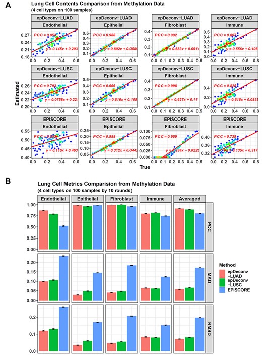
Performance comparison between epDeconv and EpiSCORE on lung cell deconvolution. (A) For the 100 DNAm simulated samples in batch 1, epDeconv-LUAD, epDeconv-LUSC and EpiSCORE perform similarly well on epithelial cells and FBs. At the same time, they show a weaker performance on the noisy endothelial and immune cells, with that of the two epDeconv models relatively good. The x-axes are the true cell contents of the simulated data and the y-axes are the estimated ones from the models, and each dot represents a simulated sample. (B) For the 10 batches of the simulated samples, epDeconv-LUAD and epDeconv-LUSC constantly perform better than EpiSCORE, from the three metrics of PCC, MAD and RMSD.
In addition, although the PCCs on epithelial cells and FBs were >0.95 for all the three methods, a difference appeared when checking the deviation of their estimates. Both epDeconv-LUAD and epDeconv-LUSC had an MAD (mean absolute deviation) value <0.05 on these two cell types, whereas for EpiSCORE, its MAD on epithelial cells was 0.146, and on FBs was 0.182, much larger than epDeconv (see Supplementary Data, Figure S3A). Besides, such a difference also appeared in RMSD (root mean squared deviation). For the endothelial and immune cells, all the methods had larger deviations. However, the epDeconv models still had an MAD and RMSD smaller than EpiSCORE.
Furthermore, this performance difference was not only in these batch 1 samples but also in all the 10 batches (Figure 2B, also see Supplementary Data, Table S1). The averaged PCC across all the four cell types and the 10 batches was 0.912 for epDeconv-LUAD. Then, the PCC for epDeconv-LUSC was 0.891, whereas that for EpiSCORE was 0.804. For the averaged MAD and RMSD, their values for epDeconv-LUAD and epDeconv-LUSC were still smaller than EpiSCORE.
This advantage of epDeconv was understandable because it leveraged more information by including the matched RNA-DNAm data. For EpiSCORE, it depended on its internal model to impute a DNAm reference from the scRNA-seq data, and the performance of this imputation was important. For epDeconv, whether the scRNA-seq data could deconvolve the paired RNA data successfully was critical because this RNA deconvolution and the DNAm deconvolution were trained together and influenced each other. Because epDeconv used the function scDeconv to conduct this RNA deconvolution, we used several RNA simulated samples to check its effectiveness. These simulated samples were synthesized from the four lung cell types in a human scRNA-seq dataset.
In detail, scDeconv first used the mouse lung scRNA-seq data to generate the reference and then used it to deconvolve the human lung RNA simulated samples, with 10 batches, and each batch contained 100 samples. In addition, the other RNA devolution method RPC used in the EpiSCORE study was also applied to these samples, but unlike scDeconv, RPC could not generate reference by itself, so EpiSCORE was used to generate an RNA reference matching its requirements. Then, their performances were compared.
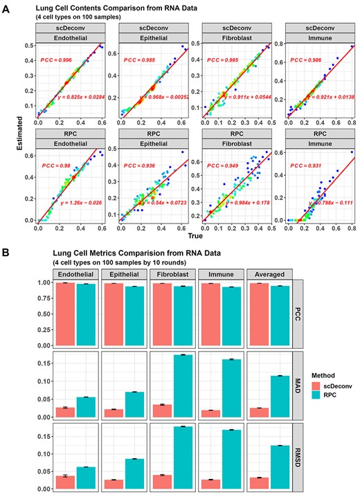
Performance comparison between scDeconv and RPC. (A) For the 100 RNA simulated samples in batch1, scDeconv and RPC perform similarly well on all four cell types. The x-axes are the true cell contents of the simulated data and the y-axes are the estimated ones from the models, and each dot is a simulated sample. (B) For the 10 batches of the simulated samples, scDeconv and RPC have similar PCCs, but the MAD and RMSD of scDeconv are better than RPC.
For the 100 RNA simulated samples in batch 1, both two methods achieved an estimates-true contents PCC >0.9 (Figure 3A). However, when checking the deviation, scDeconv showed much smaller MAD and RMSD (see Supplementary Data, Figure S3B). Its MAD values across the four cell types were ≤0.0374, and its RMSDs were ≤0.042. In contrast, the MADs of RPC were ≥0.0567, and its RMSDs were ≥0.0631. Hence, scDeconv performed better than RPC.
This conclusion could also be made on all the 10 RNA sample batches (Figure 3B, also see Supplementary Data, Table S2). For scDeconv, its averaged PCC across the four cell types, and the 10 batches was 0.987, whereas that of RPC was 0.945. However, for MAD and RMSD, their averaged values on scDeconv were much smaller than RPC.
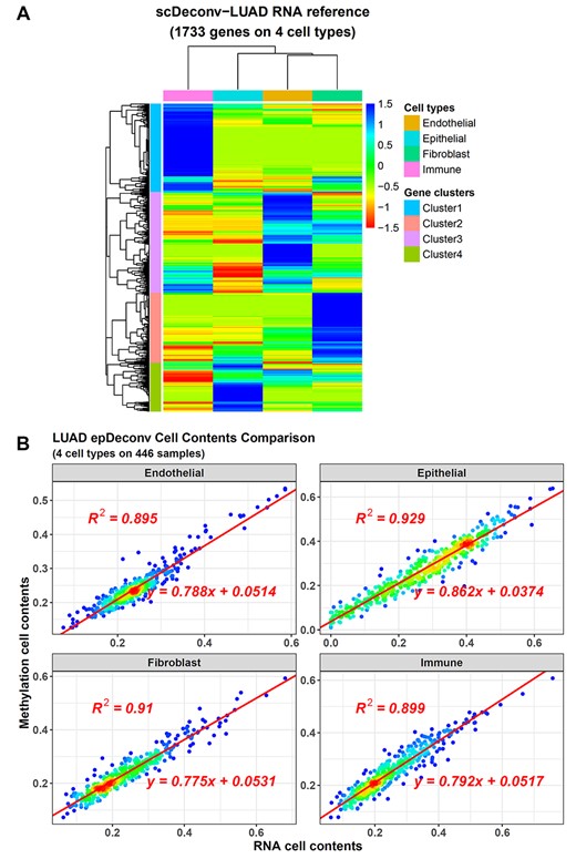
The deconvolution result on LUAD RNA samples highly correlates to the paired DNAm one. (A) The RNA reference from the epDeconv-LUAD model. (B) The paired RNA and DNAm data have similar cell deconvolution results from the epDeconv-LUAD model. The x-axes are the cell contents estimated from the RNA ensemble model and the y-axes are the ones from the paired DNAm ensemble model, and each dot is a donor with paired data.
In addition, we also selected other three scRNA-seq-based bulk RNA deconvolution algorithms (CIBERSORTx, DWLS and MuSiC) to check their performance on this dataset and found that they performed weaker than scDeconv (see Supplementary Data, Figure S4) [14, 16, 18].
This accuracy of scDeconv on RNA data was important to the epDeconv models. During the model training, scDeconv first generated the scRNA-seq-based reference and then used it to deconvolve the paired RNA data. Meanwhile, the paired DNAm deconvolution model was co-trained with this RNA model. When checking the RNA references that scDeconv generated for epDeconv-LUAD and epDeconv-LUSC, we found they largely overlapped (see Supplementary Data, Figure S5A). Among the 1733 genes in the epDeconv-LUAD reference, 1488 were shared with epDeconv-LUSC. Then, hierarchical clustering separated its genes into four clusters. Each of them showed an expression bias to one of the four lung cell types (Figure 4A). Enrichment analysis also showed matched gene functions (see Supplementary Data, Figure S6).
Because the RNA and DNAm deconvolution models were constructed under the assumption that paired samples had similar cell compositions in a co-training manner, the paired cell contents predicted by them showed a high correlation. For the four cell types in epDeconv-LUAD, their R squares were from 0.895 to 0.929 (Figure 4B), whereas that of epDeconv-LUSC were from 0.843 to 0.899 (see Supplementary Data, Figure S5B). Finally, the model was transferred to the DNAm simulated data above, and its accuracy demonstrated the correctness of this method.
This case study showed the power of scDeconv and epDeconv, and the model’s accuracy proved the ‘paired samples-similar cell contents’ assumption.
In contrast, if paired samples had very different cell contents, such as when the sample pairing was mislabeled, the basis of the model would be destroyed, and the model would not perform well. This was demonstrated by the paired sample shuffling and swapping experiments in Supplementary Data. If sampling several donors in the paired dataset and mispairing their RNA and DNAm samples, these mismatched samples would reduce the model performance. As the proportion of such mismatches increased in the dataset, epDeconv-LUAD showed a PCC decrease from 0.91 to 0.786 (mismatch proportion = 0.25), then to 0.645 (proportion = 0.5) and finally 0.00987 (mismatch proportion = 1; see Supplementary Data, Figure S7A). The epDeconv-LUSC model showed a similar trend.
In addition, we randomly paired the LUAD RNA data with the LUSC DNAm data and vice verses, and such mispaired samples also could not activate epDeconv, because they violated the ‘paired samples-similar cell contents’ law.
Besides, we checked the influence of paired sample size on the model. As the pair size decreased, the model performance became weaker, but this process was slow. For epDeconv-LUAD, when the pair size decreased from 446 to 300, the model PCC decreased from 0.91 to 0.838, then to 0.818 (pair size = 200) and finally 0.569 (pair size = 50; see Supplementary Data, Figure S7B). Also, epDeconv-LUSC showed a similar trend.
Finally, we checked the influence of DNAm platform difference on the model performance. As described in Supplementary Data, when the paired DNAm data were Illumina microarray beta values, whereas the data to be deconvolved were synthesized from scBS-seq read counts, the model could still deconvolve the cells successfully (see Supplementary Data, Figure S8).
The algorithm deconvolves whole blood leukocytes accurately
In addition to the lung cell types with a significant difference in their transcriptomic and DNAm profiles, we also tested the package on six human whole blood leukocyte cell types with much more similarity, including B cells, CD4 T cells, CD8 T cells, NK cells, monocytes and neutrophils. The bulk DNAm data to be deconvolved were simulated human blood leukocytes data with pre-defined cell compositions, and 10 batches of 100 such samples were used. As to the scRNA-seq dataset, a mouse one was used because it contained neutrophils that were always absent in human scRNA-seq datasets [19]. The blood leukocyte cell types in it were determined via cell marker expression (see Supplementary Data, Figure S9). Then, the scRNA-seq data were used by epDeconv and EpiSCORE to deconvolve the simulated data.
For the paired RNA-DNAm data needed by epDeconv, they were synthesized as described in Supplementary Data, so that three different types of data were generated for the same 100 samples, including bulk RNA-seq, bulk RNA microarray and DNAm data. The DNAm data were first paired with the bulk RNA-seq ones and transferred to epDeconv, and the resulting model was called epDeconv-RNAseq. In addition, the DNAm data were also paired with the RNA microarray data, and then an epDeconv-RNAarray model was generated. These paired data were synthesized with pre-defined cell contents so that the model performance on them could be checked, whereas the other purpose was to check the difference between using RNA-seq and microarray data as paired RNA ones.
However, from the deconvolution results on the simulated samples in batch 1, there was little difference between epDeconv-RNAseq and epDeconv-RNAarray. On the other hand, both showed a better performance than EpiSCORE (Figure 5A). For four of the six cell types (CD4 T cells, monocytes, neutrophils and NK cells), epDeconv-RNAseq achieved a true-estimated contents PCC >0.94. Meanwhile, epDeconv-RNAarray reached a level >0.86. However, EpiSCORE’s best PCC was 0.662 for neutrophils, and for the other three cell types, the PCCs were ~0.4. As to B cells and CD8 T cells, they were difficult for all the three models, and epDeconv-RNAseq had a PCC of 0.79 for B cells, and that for CD8 T cells was 0.591. For epDeconv-RNAarray, although it obtained a high PCC for B cells as 0.903, its PCC for CD8 T cells was 0.508. However, these performances were still better than EpiSCORE because it estimated these cell contents as 0 for all the samples.
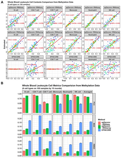
Performance comparison between epDeconv and EpiSCORE on whole blood leukocyte cell deconvolution. (A) For the 100 DNAm simulated samples in batch 1, epDeconv-RNAseq and epDeconv-RNAarray perform similarly well on CD4 T cells, monocytes, neutrophils and NK cells. At the same time, they show a weaker performance on B cells and CD8 T cells. However, all their deconvolution results are better than EpiSCORE. The x-axes are the true cell contents of the simulated data and the y-axes are the estimated ones from the models, and each dot represents a simulated sample. (B) For the 10 batches of the simulated samples, epDeconv-RNAseq and epDeconv-RNAarray perform much better than EpiSCORE, from the three metrics of PCC, MAD and RMSD. Because EpiSCORE constantly estimates the cell contents of B cells and CD8 T cells as 0, the PCCs for these two cell types cannot be calculated. So the averaged PCC across the cell types for EpiSCORE are averaged from the other four cell types, not as the two epDeconv methods from all the six cell types.
We also checked MAD and RMSD, and for batch 1, the averaged MAD value across the six cell types was 0.0365 for epDeconv-RNAseq, 0.055 for epDeconv-RNAarray and 0.161 for EpiSCORE (see Supplementary Data, Figure S10). For RMSD, its averaged value was 0.0458 for epDeconv-RNAseq, 0.067 for epDeconv-RNAarray and 0.182 for EpiSCORE.
These three models’ performance was similar for all the 10 simulated batches (Figure 5B, also see Supplementary Data, Table S3). We checked the averaged PCC; its value for epDeconv-RNAseq was 0.868, for epDeconv-RNAarray was 0.839. For EpiSCORE, the averaged PCC could only be calculated when B cells and CD8 T cells were excluded because of its constant 0 estimates on them, and even so, the averaged PCC was only 0.515. For MAD and RMSD, their averaged values for epDeconv-RNAseq and epDeconv-RNAarray were much smaller than EpiSCORE.
It was noteworthy that the performance of EpiSCORE might be underestimated here. In its original study, it was used to deconvolve five of the six blood leukocyte cell types with neutrophils excluded, starting from a human scRNA-seq dataset, and an enhancer imputation step was added to its standard pipeline to improve the performance [17]. However, in the published EpiSCORE package, we only found the standard pipeline without enhancer imputation, so this step could not be included here. Besides, the human leukocyte scRNA-seq data used in the original EpiSCORE study underwent a strict pre-selection process to improve its quality. This made its cell number reduced sharply from ~70 000 to ~15 000. In contrast, for the scRNA-seq data used here, we only processed them with the usual Seurat pipeline. These differences might lead to the reduced performance of EpiSCORE.
However, filtering the scRNA-seq data to construct a high-quality reference was legit. Hence, for the above mouse scRNA-seq dataset, we next performed a strict pre-selection process on it, following the method used in the EpiSCORE study, as described in Supplementary Data. After obtaining this super clean scRNA-seq dataset (see Supplementary Data, Figure S11A), we transferred it to epDeconv and EpiSCORE. However, we did not find much difference in the model performance. For EpiSCORE, its averaged PCC for the 10 batches improved from 0.515 to 0.534, MAD improved from 0.161 to 0.146 and RMSD improved from 0.182 to 0.167 (see Supplementary Data, Figure S11B). The two epDeconv models also showed little change. The reason might be that the usual Seurat pipeline plus manual annotation method originally used on the scRNA-seq data had already made it relatively clean because we found the original cell-type labels had a large consistency with the results of an in silico cell-type annotation (17 993/19 303 = 93.2% of the cells showed such a consistency). Hence, although the strict filtering process removed many cells and retained a super clean dataset, the deconvolution difference was small.
For the epDeconv models, the accuracy of their results demonstrated their power. In addition, their performance on the paired RNA-DNAm data used during model training was also checked because these internal data had pre-defined cell contents. For epDeconv-RNAseq, its RNA deconvolution model had a PCC >0.9 for five of the six leukocyte cell types in the paired RNA data, with CD8 T cell as an exception and its PCC was 0.624 (see Supplementary Data, Figure S12A). Its paired DNAm deconvolution model showed a similar result (see Supplementary Data, Figure S12B). This weakness in the internal CD8 T cell estimation was consistent with the weakness in the external CD8 T cell estimation above. However, B cells were estimated very well on the internal paired data. The RNA data had a PCC on B cells as 0.962, and the DNAm data had a PCC of 0.974, but it was reduced to 0.79 for the former external data. Hence, the weakness of CD8 T cells and B cells in the external data had different causes. For CD8 T cells, it was because the model itself was not trained well. For B cells, the reason should be the batch difference between the paired DNAm data and the simulated DNAm data to be deconvolved, and although ComBat was used to relieve this problem [20], it did not rescue B cells. The epDeconv-RNAarray model had a similar performance on its internal paired data (see Supplementary Data, Figure S13).
This case study showed the power of epDeconv on similar cell types and pointed out the direction to further improve the model performance.
In addition, we noted that some reference-free algorithms were developed specially for blood leukocyte DNAm deconvolution, such as methylCC [21]. It could not be used for other cell types or omics, but because it focused on the specific DNAm characteristics of blood leukocytes, the performance on these cells was highly accurate. Hence, we compared epDeonv-RNAseq and methylCC on the leukocytes DNAm data here (see Supplementary Data, Figure S14). Indeed, the averaged PCC of methylCC was higher than epDeconv-RNAseq (0.982 versus 0.868). However, its MAD was weaker than epDeconv-RNAseq (0.0437 versus 0.0369), and its RMSD was also weaker (0.0496 versus 0.0462). Hence, scDeconv kept its advantage on deviation, and meanwhile, it was a general method able to deconvolve more cell types and omics.
We also checked the scDeconv performance on leukocyte RNA data deconvolution and compared its result with other RNA deconvolution algorithms (RPC, CIBERSORTx, DWLS and MuSiC), and scDeconv still showed the best performance (see Supplementary Data, Figures S15 and S16).
Moreover, the paired sample shuffling and paired sample size experiments were also conducted for this leukocyte case (see Supplementary Data, Figure S17). However, pair size showed little influence on model performance this time. For epDeconv-RNAseq, as the pair size decreased sharply from 100 to 10, its averaged PCC decreased slightly from 0.872 to 0.782. The reason might be that the simulated RNA-DNAm sample pairs here had the same cell contents, not just similar cell contents. Hence, if the paired samples were from homogenous tissues, such as normal tissues, their cell contents tended to have more similarity and a small pair size could activate the model. In contrast, for paired samples from heterogeneous tissues, such as cancer tissues, the similarity could be reduced, so a large pair size was more reliable to ensure the performance.
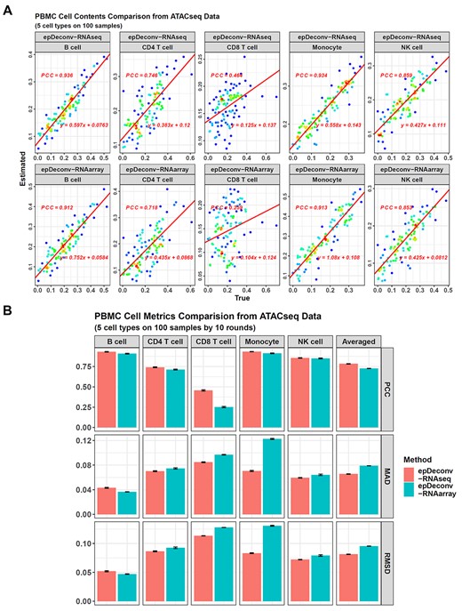
Performance of epDeconv on PBMC ATAC-seq data deconvolution. (A) For the 100 ATAC-seq simulated samples in batch 1, epDeconv-RNAseq and epDeconv-RNAarray perform similarly well on four of the five PBMC cell types, but show a weaker performance on CD8 T cells. The x-axes are the true cell contents of the simulated data and the y-axes are the estimated ones from the models, and each dot represents a simulated sample. These samples are synthesized via sampling single cells from an scATAC-seq dataset, and then mixing the cells. The true cell contents for a sample are calculated by dividing the numbers of specific cell types by the total cell number in the simulated sample. (B) For the 10 batches of the simulated ATAC-seq samples, epDeconv-RNAseq shows an averaged PCC = 0.783, MAD = 0.0655, RMSD = 0.0814, and epDeconv-RNAarray shows an averaged PCC = 0.727, MAD = 0.0789, RMSD = 0.0954.
Finally, because several scATAC-seq datasets could be found for five of the six leukocyte cell types, with neutrophils excluded, we used them to synthesize several simulated bulk ATAC-seq samples and used epDeconv to deconvolve them. As described in Supplementary Data, we synthesized a bulk RNA-seq-ATAC-seq pair dataset for the five cell types and also a bulk RNA microarray-ATAC-seq pair dataset for them. Then, we used these ATAC-seq pairs and the former mouse scRNA-seq data to train epDeconv models, and so the models were guided for ATAC-seq deconvolution rather than DNAm deconvolution. When the models were used on the simulated bulk ATAC-seq data, both showed a successful deconvolution result, and the averaged PCC across 10 batches was 0.783 for epDeconv-RNAseq, and 0.727 for epDeconv-RNAarray (Figure 6, also see Supplementary Data, Table S4). Hence, in addition to RNA and DNAm, scDeconv could also deconvolve other omics.
It was noteworthy that the simulated ATAC-seq data to be deconvolved were synthesized via sampling single cells from an external scATAC-seq dataset and then mixing the cells. Hence, the variance among different single cells was included in the synthesized bulk ATAC-seq samples, which was more similar to the data in the real world.
The algorithm deconvolves placenta cells accurately
We also used the package to deconvolve a human placenta DNAm dataset collected from various studies. After data preprocessing and combination, we only kept the probes with high data quality and covered by both the Illumina 27K and 450K platforms. The final dataset contained 18 626 probes and 359 samples, and 48 of them had corresponding RNA microarray data, whereas the other 311 only had DNAm measurements. All the 48 sample pairs were from the GEO (Gene Expression Omnibus) dataset GSE98224 and included 18 normal pairs and 30 disease sample pairs with the preeclampsia pregnancy complication. Hence, we used GSE98224 as the paired RNA-DNAm dataset to train the model. Meanwhile, the 311 single DNAm samples were the bulk DNAm data to be deconvolved, including 240 normal placenta samples and 71 preeclampsia ones. The scRNA-seq data needed to construct the reference was from a human placenta scRNA-seq study.
Based on these resources, we used epDeconv to calculate the contents of four placental cell types, including extravillous trophoblast (EVT), fibroblast (FB), Hofbauer cell (HB) and villous cytotrophoblast (VCT). EVT and VCT were epithelial trophoblasts with similar origins, whereas HB cells were fetal macrophages present in the placenta.
The paired RNA and DNAm samples’ deconvolution results from epDeconv showed a high correlation (Figure 7A). Moreover, if split the cell contents into normal and preeclampsia groups, the paired RNA and DNAm samples also showed a similar inter-group difference (Figure 7B and C), with EVT cells upregulated in preeclampsia, whereas HB and VCT cells downregulated. When the model was applied to the final bulk DNAm data to be deconvolved, it also showed this inter-group difference (Figure 7D).

Cell deconvolution results on placenta DNAm samples. (A) For the four placental cell types, their deconvolution results for the paired RNA and DNAm data show a high correlation. The x-axes are the cell contents calculated from the RNA samples and the y-axes are for the DNAm ones, and each dot is a donor with paired data. (B) and (C) The RNA (B) and the DNAm (C) samples show a similar cell content difference between normal and preeclampsia groups. (D) Cell deconvolution results on all the DNAm samples, including the paired DNAm samples and the non-paired ones, show an essentially dynamic status of placental cell composition.
We validated the deconvolution results for the paired samples via the known cell marker genes, which were expected to correlate with the cell contents significantly. For the four cell types, we calculated the PC1 (first principle component) values of their known marker genes in the paired RNA data. In the paired RNA samples, the deconvolution results significantly correlated to these cell-type marker PC1s, with EVT, FB and HB cells showing a PCC >0.7 and VCT obtaining one of 0.663 (see Supplementary Data, Figure S18A). For the paired DNAm samples, their cell contents also correlated with these RNA marker PC1s, still with a PCC >0.7 on the former three cell types and a PCC >0.6 on VCT (see Supplementary Data, Figure S18B).
In addition, the control and preeclampsia cell composition difference was consistent with previous reports, which validated the deconvolution indirectly. For example, several studies had reported an HB cell reduction in preeclampsia. Its significance was to promote inflammatory damage in this disease due to the loss of tolerance-promoting HB cells [22–24]. Meanwhile, an immunohistochemical study had proved the increase of EVT cells. It had shown that preeclampsia samples had more immature EVT cells [25]. In addition, Longtine et al. had observed that VCT cells underwent elevated apoptosis in this disease, consistent with their decreased cell contents in preeclampsia revealed here [26].
After this deconvolution, we used the cell composition of all the 359 samples to identify cell-type-specific inter-group differential DNAm sites from these bulk DNAm data, which was fulfilled by the function celldiff in the package. As described in Supplementary Data, it identified these cell-type-specific sites via a linear model with an interaction term between the disease status and cell contents. The results showed that all four cell types had several hyper and hypomethylated sites in the disease condition (see Supplementary Data, Figure S19).
To validate that these CpG sites were really cell-type-specific, we used the tool eFORGE [27], which detected enrichment of CpG sites mapped to cell-type-specific DHSs (DNase I hypersensitive sites). For example, if the FB-specific CpG sites identified by celldiff were correct, they should be enriched in corresponding FB DHSs, and the same for EVT, HB and VCT cells. Besides, we applied another tool, TCA, on the placenta dataset because it was also designed to identify cell-type-specific CpG sites from bulk tissue data and cell contents [28].
From eFORGE, all the probe sets identified by celldiff showed significant enrichment in corresponding tissue-specific or cell-type-specific DHSs (see Supplementary Data, Figure S20). However, for TCA, only two of its four probe sets showed significant enrichment. Hence, celldiff performed better than TCA.
After validating these celldiff identified probes, another function, enrichwrapper, was used to find their enriched functions. It utilized the paired RNA-DNAm data again to identify genes with an RNA expression significantly correlated to the differential DNAm probes and then used these genes to perform the functional analyses. Compared with the traditional methods directly on hyper and hypomethylated genes, this correlation step removed those whose DNAm change has little influence on their gene expression and thus avoided their misleading effects.
The identified functions were well related to the disease (see Supplementary Data, Figure S21). For example, in HB cells, ‘Purine catabolism’ was revealed as an enhanced pathway in preeclampsia. On the other hand, this disorder was always coupled with a higher uric acid level, a product of purine catabolism [29]. In VCT cells, ‘Telomere extension by telomerase’ was prompted, consistent with an increased telomerase level in preeclampsia [30]. In EVT cells, the ‘Leukotriene receptors’ pathway was upregulated. Due to their roles as inflammatory mediators, it was consistent with the inflammatory stress of preeclampsia [31].
This case study showed a comprehensive application of the package.
Discussion
DNAm is an epigenetic mark associated with various pathological conditions [2, 3]. However, due to cost and other reasons, most DNAm profiles have been generated from tissues with multiple cell types, preventing the identification of cell-type-specific changes underlying disease. Hence, cell deconvolution on bulk DNAm data becomes vital.
Compared with RNA deconvolution, DNAm deconvolution has a bottleneck: the cell-type-specific DNAm references are limited. Hence, a computational method to solve it is meaningful.
One thought is to convert scRNA-seq data and make them usable for DNAm deconvolution. This is the motivation to develop scDeconv. To fulfill it, scDeconv utilizes additional paired bulk RNA-DNAm data. It assumes the paired samples have similar cell compositions, so the cell contents deconvolved from the scRNA-seq, and the paired RNA data can be transferred to the DNAm data and used as their true labels to train a model from DNAm features.
It is noteworthy that the model selects DNAm features to fit the cell contents rather than the gene expression levels, so it selects not only the features contributing to gene expression but also those without a clear relationship to genes but correlated to cell contents. Hence, compared with EpiSCORE, which depends on the DNAm-gene expression relationship, scDeconv selects more DNAm features and obtains more information.
However, also because of the more features, the running time of scDeconv is longer than EpiSCORE. So in the lung and blood leukocyte cases, we summarized the methylation probes to gene level before running epDeconv to reduce the candidate feature number and accelerate it. Then, after scRNA-seq reference generation, with six threads, epDeconv took 3 min to complete the lung or leukocyte dataset deconvolution, whereas in the condition of no parallelization, EpiSCORE could finish the deconvolution within 30 s. The other shortcoming of scDeconv is its requirement for the paired RNA-DNAm data, which needs users to spend additional time finding them. However, for the model performance, scDeconv shows a significant advantage.
scDeconv is an R package to deconvolve bulk DNAm data with scRNA-seq data and paired RNA-DNAm data in a trans-omics manner.
scDeconv outperforms other algorithms in both single-omics and trans-omics deconvolution.
If given an appropriate paired dataset, scDeconv can also deconvolve other omics, such as ATAC-seq data.
scDeconv finds cell-type-specific inter-group differential features from bulk DNAm data effectively.
