


Abstract
Effective computational methods to predict drug–protein interactions (DPIs) are vital for drug discovery in reducing the time and cost of drug development. Recent DPI prediction methods mainly exploit graph data composed of multiple kinds of connections among drugs and proteins. Each node in the graph usually has topological structures with multiple scales formed by its first-order neighbors and multi-order neighbors. However, most of the previous methods do not consider the topological structures of multi-order neighbors. In addition, deep integration of the multi-modality similarities of drugs and proteins is also a challenging task.
We propose a model called ALDPI to adaptively learn the multi-scale topologies and multi-modality similarities with various significance levels. We first construct a drug–protein heterogeneous graph, which is composed of the interactions and the similarities with multiple modalities among drugs and proteins. An adaptive graph learning module is then designed to learn important kinds of connections in heterogeneous graph and generate new topology graphs. A module based on graph convolutional autoencoders is established to learn multiple representations, which imply the node attributes and multiple-scale topologies composed of one-order and multi-order neighbors, respectively. We also design an attention mechanism at neighbor topology level to distinguish the importance of these representations. Finally, since each similarity modality has its specific features, we construct a multi-layer convolutional neural network-based module to learn and fuse multi-modality features to obtain the attribute representation of each drug–protein node pair. Comprehensive experimental results show ALDPI’s superior performance over six state-of-the-art methods. The results of recall rates of top-ranked candidates and case studies on five drugs further demonstrate the ability of ALDPI to discover potential drug-related protein candidates.
1 Introduction
Predicting drug–protein interactions (DPIs) is an important step in drug discovery and repositioning [1–3]. Accurately and effectively identifying the interactions between drugs and targets can facilitate the drug development process and reduce the required time and cost [4, 5]. Computational prediction of novel DPI candidates may screen potential candidates for biologists to discover the true DPIs using experiments [6].
Early methods, including ligand-based and molecular docking, have been proposed to predict DPIs. Ligand-based approaches compare similarities between candidate ligand and the known ligands of a target protein, and then estimate the possibility that the candidate ligand binds to the protein [7, 8]. Docking simulation methods utilize the 3D structure of the protein and dynamically simulate them to assess the affinity of the interaction between drug molecules and proteins [9, 10]. However, these methods are severely limited by the unknown 3D structure and ligand information of most proteins [11–13].
Recent studies have shown that machine learning methods are more effective and achieve better performance in predicting DPI [14, 15]. These methods can be divided into four main categories namely: biological characteristic-based, similarity-based, network-based and deep learning-based. In the biological characteristic-based methods, Ding et al. [16] extracted the characteristics of drugs and proteins from drug molecular fingerprints and protein amino acid sequences. They then applied a support vector machine (SVM) model to predict DPIs. Chu et al. [17] introduced multi-label learning and community detection to the task and used random forest for prediction. Two methods [18, 19] fed the drug structures and protein sequences into a rotation forest-based model to evaluate the DPI tendency. Similarity-based methods are proposed based on the assumptions that if drug |$r$| interacts with protein |$p$|, then (i) drug |$r$| is likely to interact with proteins that are similar to |$p$|, (2) protein |$p$| is likely to interact with drugs that are similar to |$r$| and (iii) drugs similar to |$r$| are likely to interact with proteins similar to |$p$|. Ezzat et al. [20] used chemical structure similarities of drugs and sequence similarities of proteins and DPIs to establish a matrix factorization framework. They also proposed weighted |$k$| nearest known neighbors as a preprocessing step to estimate the interaction possibility of unknown cases. Several methods combine drug similarity and protein similarity and predict novel interaction candidates by SVM, principal component analysis (PCA), Gaussian kernel model and matrix factorization [21–24]. They used only one type of drug similarity and protein similarity. However, the types of similarities were diverse. Olayan et al. [25] and Xuan et al. [26] integrated multiple similarities between drugs and proteins and applied random forest and gradient boosting decision trees to obtain drug–protein interaction scores, respectively. DTI-CDF (cascade deep forest) [27] also extracted hybrid similarity features of drugs and proteins and predicted them using a cascade deep forest model. Because the topology of heterogeneous networks may also assist in DPI prediction, network-based methods have gained wider attention. Bleakly et al. [28] and Mei et al. [29] established a common bipartite local model for prediction. Luo et al. [30] first constructed a drug–protein heterogeneous network based on several types of drug- and protein-associated connections. They then applied singular value decomposition to learn feature vectors containing topological information of nodes and predicted novel DPIs. However, the models mentioned above are shallow prediction models, which are unable to learn deep features from related data and capture potential connections in the network.
Deep learning techniques have proven to be powerful predictors in many fields. Recently, deep learning-based methods have been used to predict DPIs. Lee et al. [31] constructed deep neural network (DNN) model to capture the local residue patterns of proteins participating in DPIs. Specifically, they performed convolution operations on different lengths of sequences to capture local features. Wang et al. [32] utilized PCA to learn drug- and protein-related feature matrices and predicted by the long short-term memory model. They ignored important similarity information. Sun et al. [33] combined similarities data and preserved the consistency of the features and functions of drugs. Several other methods integrated multiple similarities between drugs and proteins and predict novel interactions by convolutional neural network (CNN), fully connected autoencoder and gated recurrent unit (GRU) models [34–36]. In addition, graph neural network-based methods also consider topological information and node features in graph. Sun et al. [37] developed a prediction model based on graph convolution and generative adversarial network using a single type of drug and protein similarity. Zhao et al. [38] first constructed a heterogeneous network using drug-protein pairs as nodes. They then learned node features using graph convolutional networks and predicted DPI using DNNs. Although the above works have made crucial efforts in DPI prediction, there are still some spaces that can be improved.
In this study, we propose a model called ALDPI to predict novel drug–protein interactions. The model learns the topological representation in a drug–protein heterogeneous graph and integrates the multi-modality similarities of drugs and proteins. The main contributions of our model are described as follows:
We calculated multi-modality similarities of drugs and proteins based on different source data, and these similarities reflect how similar two drugs (two proteins) are from different views. We then utilized interactions between drugs and proteins and multi-modality similarities of drugs and proteins to construct the drug–protein heterogeneous graph.
To deeply integrate the multi-order neighbor topology information of nodes in the graph, we propose an adaptive topology graph learning module. The module softly selects the weights of the different connected edges to generate multiple new topology graphs.
A module based on graph convolution autoencoder is constructed to learn the multiple topology representations of nodes based on different order neighbor topologies. Since these topology representations have different importance for DPI prediction, we further establish a neighbor topology-level attention mechanism to discriminate the importance and obtain an enhanced topology representation of node.
We designed a multi-layer CNN-based strategy to deeply integrate the multi-modality similarities of drugs and proteins. The specific modality attribute learning module learns specific features from different modality similarities, and these features are integrated by the convolution layer to form the attribute representation of the node pair. The results of the evaluation metrices show that our model is superior to the six state-of-the-art methods, and the case studies prove the ability of ALDPI to predict potential drug–protein interactions.
2 Materials and method
2.1 Overview of ALDPI
We propose a novel deep learning model called ALDPI that combines multi-order neighbor topologies and multi-modality similarities of drugs and proteins for DPI prediction. The pipeline of the ALDPI method is shown in Figures 1 and 2. First, we construct the drug–protein heterogeneous graph based on drug- and protein-related interactions and multiple types of similarities (Figure 1). Then, the topology representations of nodes and the attribute representations of drug–protein node pairs are learned, respectively (Figure 2A and B). Finally, we combine these two representations to estimate the interaction score of a pair of drug and protein (Figure 2C).
2.2 Dataset
The dataset from Luo et al. [30] contains 708 drugs extracted from the DrugBank database [39], 1512 proteins from the Human Protein Reference Database (HPRD) [40] and 5603 diseases from the Comparative Toxicogenomics Database (CTD) [41]. We collect the latest drug–protein interaction (DPI) data from DrugBank to update the dataset. We remove drugs and proteins without DPIs and diseases that are not associated to drugs and proteins. There are 570 drugs, 467 proteins and 5420 diseases. The latest dataset provides corresponding 2816 DPIs and 7016 drug–drug interactions (DDIs) from DrugBank, 1452 protein-protein interactions (PPIs) from HPRD, 178 477 drug-disease associations and 544 437 protein-disease associations from CTD. In addition, the chemical structure similarity of drugs is the Tanimoto coefficient of the product-graphs of their chemical structures, and the sequence similarity of the proteins is calculated using Smith-Waterman score based on their amino acid sequences.
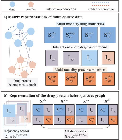
Matrix representations of multi-source data and construction of the drug–protein heterogeneous graph. (A) matrix representations of multi-source data including multi-modality similarities and interactions about drugs and proteins. (B) adjacency relationship and attribute representations of drug–protein heterogeneous graph.
2.3 Matrix representation of multi-source data and heterogeneous graph construction
2.3.1 Matrix representation of interactions and associations
Suppose there are |$N_r$| drug nodes, denoted as |$V_R= \{r_1,r_2,\ldots ,r_{N_r} \}$|, |$N_p$| protein nodes, denoted as |$V_P= \{p_1,p_2,\ldots ,p_{N_p} \}$| and |$N_d$| disease nodes, denoted as |$V_D= \{d_1,d_2,\ldots ,d_{N_d} \}$|. We defined interaction matrix |$\bf{I}$| and association matrix |$\bf{A}$| according to the connection relationships (interaction or association).
2.3.2 Matrix representation of multi-modality similarities
2.3.3 Construction of drug–protein heterogeneous graph
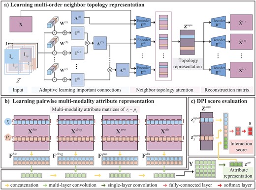
The pipeline of the proposed ALDPI method for DPI prediction. Given drug |$r_i$| and protein |$p_j$|, two types of representations are learned by (A) topology representation learning module based on convolution operations, graph convolutional autoencoder and neighbor topology-level attention and (B) attribute representation learning module consist of CNN. Finally, (C) topology and attribute representation are integrated to estimate the interaction score of |$r_i-p_j$|.
2.4 Capturing graph topology and learning node feature
Facing the drug–protein heterogeneous graph, we establish a topology graph learning module to adaptively adjust weight of connections and obtain the multiple topology graphs. Then different topology representations of node are learned by graph convolutional autoencoders, and they contribute differently to the prediction of DPI. Therefore, N-attention (neighbor topology-level attention) is proposed to measure the attention weight of each representation.
2.4.1 Adaptive neighbor-based topology graph learning
2.4.2 Neighbor topology encoding by graph convolutional autoencoder
To learn topological representations of drug and protein nodes, the adaptive neighbor-based topology graph |$\textbf{A}^{(l)}$| and concatenate attribute matrix |$\textbf{X}$| are integrated by graph convolutional autoencoders. The representations capture topology information formed by neighbor topologies of different orders and contain attribute information of drugs and proteins.
2.5 Learning multi-modality attribute representation
The graph convolutional autoencoder modules concatenate |$\textbf{X}^{bio}$|, |$\textbf{X}^{drug}$|, |$\textbf{X}^{pro}$| and |$\textbf{X}^{dis}$| as input features and completely integrate multi-modal similarities. To learn the features of each modality similarity and distinguish their contributions, we establish a selective multi-modality attribute learning model.
2.5.1 Constructing attribute matrix of drug–protein node pair
2.5.2 Pairwise attribute feature learning
The pairwise attribute feature learning module is constructed based on a CNN, which contains the specific modality attribute learning part and the fusion part.
2.5.3 The final representation of pairwise drug–protein
2.6 Interaction score evaluation and optimization
2.6.1 drug–protein interaction prediction
2.6.2 Loss function and optimization
3 Results and discussion
3.1 Performance evaluation
To facilitate the comparison between the proposed method and other methods, we performed 10-fold cross-validation (CV) for each experiment. The 2816 known DPIs (positive samples) are divided into ten subsets. In each fold CV, the training set contains nine positive subsets and the same number of randomly selected unknown drug–protein interaction pairs, while the remaining one positive subset and the remaining unknown drug–protein interaction pairs are used for testing. Moreover, during each fold CV, the drug similarity matrix |$\textbf{S}_{rr}^{pro}$| and protein similarity matrix |$\textbf{S}_{pp}^{drug}$| are recalculated according to the drug–protein interactions in the training set.
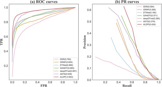
The comparison of the ALDPI with other six state-of-the-art methods in AUC and AUPR. (A) ROC curves of different DPI prediction methods. (B) PR curves of different DPI prediction methods.
3.2 Implementation and parameter settings
Our method ALDPI is implemented by Python on an Nvidia GeForce GTX 2080Ti graphic card with 11G graphic memory. In the adaptive topology graph learning module, the layer of |$1\times 1$| convolution is set 3. For the graph convolutional autoencoder-based module, the number of encoding layers and decoding layers is 2, the dimensions of node embedding are 1024 and 256 after the first encoder layer and the second encoder layer, respectively. In the multi-layer CNNs, the filter size of the former two layers is |$3\times 5$|, and the filters size of the last layer is |$4\times 5$|. The learning rates of the graph convolutional autoencoder-based module and CNN are set as 0.001 and 0.0001, respectively.
3.3 Comparison with other methods
Six state-of-the-art methods in comparison include AEFS [33], deepDTnet [35], GANDTI [37], DTINet [30], GRMF [20] and DDR [25]. For fair comparison, the hyperparameters in comparison model are set by the recommended range of the corresponding literature. (|$\lambda _{1}=0.001$|, |$\lambda _{2}=0.01$|, |$\lambda _{e}=2$|, |$\lambda _{d}=2$| for AEFS; |$\alpha =0.8$|, |$lr=0.001$| for deepDTnet; |$l=512$|, |$k=256$|, |$lr=0.005$| for GANDTI; |$r=0.8$|, |$n=10$| for DTINet; |$\eta =0.5$|, |$\lambda _{d}=0.1, \lambda _{t}=0.1, \lambda _{l}=2$| for GRMF; |$n=600$|, |$k=5$| for DDR.)
Figure 3 shows the average ROC and PR curves of ALDPI and other comparison methods for all the 570 drugs. ALDPI achieved the highest average AUC of 0.953, which is superior than 1.4|$\%$| by AEFS, 6.2|$\%$| by deepDTnet, 6.4|$\%$| by DTINet, 8.8|$\%$| by GANDTI, 9.8|$\%$| by GRMF and 16.1|$\%$| by DDR (Figure 3A). In terms of average AUPR over all the drugs, the best performance of 0.424 was obtained by ALDPI, which is, respectively, 4.5, 5.3, 13.4, 15.6, 24.4 and 33.0|$\%$| higher than that of AEFS, GANDTI, deepDTnet, GRMF, DTINet and DDR (Figure 3B). In addition, we also draw the ROC and PR curves of ALDPI for each fold CV, and then calculate their AUCs and AUPRs, respectively (Supplementary Figure 1). We also performed experimental comparison on the two golden datasets, including Luo’s dataset [30] and Yamanishi’s dataset [49]. The average AUCs and AUPRs of ALDPI and the compared methods are listed in Supplementary Tables 1, 2 and 3. We observed that ALDPI still achieved higher AUCs and AUPRs than other methods over Luo’s dataset and Yamanishi’s dataset, which indicates that ALDPI has good generality over various datasets.
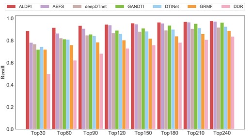
Recall rates of all method under different top |$k$|.
In order to evaluate the impact of the training set on the prediction performance, we use the datasets containing different ratios of known DTIs and unknown drug–protein interaction pairs to train ALDPI. In 10-fold CV, we divide 2816 known DPIs into 10 subsets and take 9 of them as the training set. We add different ratios of known DPIs and unknown drug–protein interaction pairs to the training set, and the experimental results are shown in Supplementary Table 4. The results show that when the ratio of the known DPIs to unknown drug–protein interaction pairs in the training set is 1:1, ALDPI achieved the best prediction performance (AUC =0.953, AUPR = 0.424). When the ratio is 1:5, ALDPI obtained the second-best performance, and AUC and AUPR decreased by 0.3|$\%$| and 1.0|$\%$|, respectively. When the ratio is 1:10, 1:20, 1:30 and 1:40, the AUC decreased by 1.8, 2.0, 2.4 and 4.5|$\%$| respectively, and the AUPR decreased by 2.6, 3.6, 2.9 and 6.8|$\%,$| respectively. The lowest AUC and AUPR of ALDPI are 0.904 and 0.337, respectively, when the ratio is 1:50. In summary, the performance of our model gradually decreased when the number of unknown drug–protein interaction pairs increased. Therefore, we choose a training set with a ratio of 1:1 to train ALDPI.
Our method ALDPI achieved the best performance in both AUC and AUPR, and the AEFS achieved the second-best AUC and AUPR.ALDPI based on the graph convolutional autoencoder and CNN could deeply integrate drug and protein-related multi-modal similarity features. AEFS encodes the features of drugs and proteins and preserves the consistency of the chemical properties and functions of drugs. Fully connected autoencoder-based deepDTnet and generative adversarial networks based GANDTI also learn deep features to predict DPI, and they also achieved good results (deepDTnet’AUC = 0.891, GANDTI’AUPR = 0.371). The AUC of DTINet was higher than that of GRMF, but its AUPR was lower 8.8|$\%$| than GRMF. DDR performed much worse than other methods, one possible reason is that it neglected the attribute information of drugs and proteins. Our finding is that the deep representation of features learned based on deep learning frameworks contributes to improving performance compared to shallow prediction models. In addition, our method ALDPI also capture multi-order topological structure of heterogeneous graph. The machine learning-based DTINet and GRMF extracted topological properties and their performance is higher DDR. The results shows that the learning topology structure information of graph is vital for the promoting prediction.
Figure 4 shows the top-k recall rates of all methods. The higher the recall rate, the more drug-related proteins could be correctly identified. Under different threshold k, ALDPI outperformed other methods and ranked 88.6% in the top 30, 91.5% in the top 60 and 93.3% in the top 90. AEFS achieved the second-best performance, with recall rates of 78.1, 86.4 and 90.7% in the top 30, 60 and 90. In the top 120–240, the recall rate of AEFS was close to that of ALDPI. The recall rates of deepDTnet and DTINet are almost the same, the GANDTI’ recall rates were lower than those in the top 30 and 60 and higher than those after the top 90. The performances of GRMF and DDR are not as good as the above methods. The recall rates of the former model in the top 30, 60 and 90 are 71.9, 75.8 and 78.4%, respectively, and those of the latter model are 49.7, 62.1 and 68.3%, respectively. In addition, we used the Wilcoxon test to evaluate whether ALDPI’s performance was better than the comparison method. The statistical results given in Table 1 indicates that the performance of ALDPI is significantly better than other methods (|${P}$| value < 0.05).
Comparion between ALDPI and other methods based on AUCs and AUPRs with the paired Wilcoxon test
| AEFS | deepDTnet | GANDTI | DTINet | GRMF | DDR | |
|---|---|---|---|---|---|---|
| |${P}$| value based on AUC | 5.2408e-16 | 2.0531e-23 | 2.0342e-05 | 3.6250e-03 | 6.7494e-04 | 1.9779e-03 |
| |${P}$| value based on AUPR | 1.7719e-03 | 3.2424e-70 | 4.7648e-79 | 4.3421e-19 | 5.5668e-28 | 2.5750e-09 |
The top 10 candidate target proteins of five drugs
| Enflurane | |||||
|---|---|---|---|---|---|
| Rank | Gene | Evidence | Rank | Gene | Evidence |
| 1 | GABRA3 | DrugBank | 6 | GABRG2 | DrugBank |
| 2 | GABRB2 | DrugBank | 7 | GABRD | DrugBank |
| 3 | GABRB3 | DrugBank | 8 | GABRA1 | DrugBank |
| 4 | GABRG3 | DrugBank | 9 | KCNQ5 | DrugBank |
| 5 | GABRA4 | DrugBank | 10 | GABRG1 | DrugBank |
| Aripiprazole | |||||
| Rank | Gene | Evidence | Rank | Gene | Evidence |
| 1 | HTR1B | DrugBank,DrugCentral | 6 | HTR2C | DrugBank,DrugCentral |
| 2 | ADRA2C | DrugBank,DrugCentral | 7 | ADRA2B | DrugBank,DrugCentral |
| 3 | HTR6 | DrugBank,DrugCentral | 8 | HTR1D | DrugBank,DrugCentral |
| 4 | HTR1A | DrugBank,DrugCentral | 9 | OPRD1 | DrugBank |
| 5 | ADRA2A | DrugBank,DrugCentral | 10 | CHRM2 | DrugBank,DrugCentral |
| Amoxapine | |||||
| Rank | Gene | Evidence | Rank | Gene | Evidence |
| 1 | ADRA1A | DrugBank | 6 | GABRG3 | DrugBank |
| 2 | HTR2C | DrugBank | 7 | ADRA1B | DrugBank |
| 3 | HTR1B | DrugBank | 8 | HMGCR | Unconfirmed |
| 4 | CHRM3 | DrugBank,DrugCentral | 9 | CHRM1 | DrugBank,DrugCentral |
| 5 | GABRB3 | DrugBank | 10 | DRD1 | DrugBank,DrugCentral |
| Amitriptyline | |||||
| Rank | Gene | Evidence | Rank | Gene | Evidence |
| 1 | CHRM1 | DrugBank,DrugCentral | 6 | HTR2C | DrugBank,DrugCentral |
| 2 | HTR1A | DrugBank,DrugCentral | 7 | CHRM5 | DrugBank,DrugCentral |
| 3 | ADRA1D | DrugBank,DrugCentral | 8 | SLC6A2 | DrugBank,DrugCentral,ChEMBL |
| 4 | HTR1D | DrugBank | 9 | ADRA1A | DrugBank,DrugCentral |
| 5 | ADRA1B | DrugBank | 10 | HTR7 | DrugBank,DrugCentral |
| Paroxetine | |||||
| Rank | Gene | Evidence | Rank | Gene | Evidence |
| 1 | ADRA2B | DrugBank | 6 | CHRM1 | DrugBank,DrugCentral |
| 2 | HTR1A | DrugBank,DrugCentral,ChEMBL | 7 | HTR1D | DrugBank |
| 3 | CHRM5 | DrugBank,DrugCentral | 8 | DRD2 | DrugBank |
| 4 | HTR1F | DrugBank | 9 | ADRA1A | DrugBank |
| 5 | HTR1B | DrugBank | 10 | ADRA2A | DrugBank |
Top 15 of predicted drug–protein pair candidates
| Rank | Drug ID | Drug name | Protein ID | Gene | Evidence |
|---|---|---|---|---|---|
| 1 | DB06710 | Methyltestosterone | P04150 | NR3C1 | DrugCentral |
| 2 | DB00624 | Testosterone | P04150 | NR3C1 | DrugCentral |
| 3 | DB00700 | Eplerenone | P04150 | NR3C1 | DrugCentral,ChEMBL |
| 4 | DB00603 | Medroxyprogesterone Acetate | P04150 | NR3C1 | DrugCentral,ChEMBL |
| 5 | DB00990 | Exemestane | P04150 | NR3C1 | Literature [48] |
| 6 | DB04839 | Cyproterone Acetate | P04150 | NR3C1 | DrugCentral |
| 7 | DB00408 | Loxapine | P25100 | ADRA1D | DrugCentral,ChEMBL |
| 8 | DB00679 | Thioridazine | P25100 | ADRA1D | DrugCentral |
| 9 | DB00910 | Paricalcitol | P04150 | NR3C1 | Unconfirmed |
| 10 | DB00334 | Olanzapine | P08912 | CHRM5 | DrugCentral |
| 11 | DB00652 | Pentazocine | P41143 | OPRD1 | DrugCentral |
| 12 | DB00187 | Esmolol | P07550 | ADRB2 | DrugCentral,ChEMBL |
| 13 | DB00247 | Methysergide | P28221 | HTR1D | DrugCentral |
| 14 | DB00334 | Olanzapine | P25100 | ADRA1D | DrugCentral |
| 15 | DB00458 | Imipramine | P08913 | ADRA2A | DrugCentral,ChEMBL |
3.4 Case studies
To demonstrate the ability of ALDPI to discover potential DPIs, we applied case studies for five drugs, namely Enflurane, Aripiprazole, Amoxapine, Amitriptyline and Paroxetine. The top 10 protein candidates for each drug are collected, with 50 candidates in total (Table 2).
First, the DrugBank [39] is a web-enabled database containing comprehensive drug data covering drug function, drug targets and so on. The DrugCentral [46] is also an online public database that provides up-to-date drug information, such as the interactions between drugs and proteins. The ChEMBL database [47] records bioactive drug-like small molecule data, which are abstracted and curated from the primary scientific literature. As shown in Table 2, 49 candidates were inferred from the DrugBank database. DrugCentral and ChEMBL contain 23 and 2 candidate proteins, respectively. It indicated that these candidate proteins are indeed interacted with the corresponding drugs.
Next, Table 3 lists the 15 drug–protein pair candidates with the highest predicted interaction scores to further verify the utility of ALDPI. The Drug Central verified 10 drug–protein pair candidates, and the ChEMBL recorded two candidates. These drugs have been confirmed to affect the corresponding proteins in humans.
In addition to the DPIs in humans confirmed by the database, several candidates were supported by literatures or experiments on animals. DrugCentral and ChEMBL verified the interactions between loxapine and ADRA1D, imipramine and ADRA2A in rattus norvegicus, and esmolol and ADRB2 in cavia porcellus. These evidences also laid the foundation for exploration of interactions in humans. In a recent study, Wang et al. [48] selected exemestane for functional validation and drug availability to treat glucocorticoid resistance. Overall, these cases further demonstrated the capability of our model is able to discover the potential candidate DPIs.
3.5 Prediction of novel drug–protein interactions
Our proposed model ALDPI is used to predict protein candidates, which are related with the drugs. All of the known DPIs are applied to train ALDPI. The top 30 ranked protein candidates and corresponding interaction scores for each drug predicted by our model are listed in Supplementary Table 5. Supplementary Table 5 may assist biologists in discovering novel drug-related proteins in wet-lab experiments.
4 Conclusion
In this study, we proposed a method ALDPI to predict candidate drug–protein interactions. The drug–protein heterogeneous graph was constructed to benefit extracting the multi-order neighbor topology structures. The proposed adaptive graph learning module can transform the heterogeneous graph into multiple new graphs with different neighbor topologies. The graph convolutional autoencoders were applied to learn the representation of nodes based on the different-order neighbor topology. The topology representation-level attention mechanism was established to assign higher weights to the more informative topological representations. The multi-layer CNN-based module was designed to learn the attribute features of different modality similarities and selectively fuse these features. Evaluated using 10-fold CV, ALDPI outperformed the state-of-the-art methods under the evaluation measures of AUC, AUPR, top-k recall values and Wilcoxon test. The case studies further proved that our model has the ability to predict novel drug–protein interactions. In conclusion, the experimental results demonstrated that ALDPI is a reliable tool for biologists to screen candidate DPIs.
A drug–protein heterogeneous graph is constructed, which benefits the extraction and representation of neighbor topology information and multi-modelity similarity attributes of nodes.
The new topology graphs obtained by the established graph learning module contain the multi-order neighbor topologies and reveal the potential connections between nodes.
A newly neighbor topology-level attention mechanism is proposed to discriminate the importance of multiple topology representations of nodes, which are learned by graph convolutional autoencoders based on different order neighbor topology graphs.
A novel strategy based on multi-layer CNNs is designed to learn the specific features corresponding to different modality similarities and then deeply integrate these features.
Funding
The work was supported by the Natural Science Foundation of China (61972135, 62172143); Natural Science Foundation of Heilongjiang Province (LH2019A029); China Postdoctoral Science Foundation (2019M650069, 2020M670939); Heilongjiang Postdoctoral Scientific Research Staring Foundation (BHLQ18104); Fundamental Research Foundation of Universities in Heilongjiang Province for Technology Innovation (KJCX201805); Innovation Talents Project of Harbin Science and Technology Bureau (2017RAQXJ094); Fundamental Research Foundation of Universities in Heilongjiang Province for Youth Innovation Team (RCYJTD201805); and the Foundation of Graduate Innovative Research (YJSCX2021-077HLJU).
Kaimiao Hu is studying for his master’s degree in the School of Computer Science and Technology at Heilongjiang University, Harbin, China. Her research interests include complex network analysis and deep learning.
Hui Cui, PhD (The University of Sydney), is a lecturer at Department of Computer Science and Information Technology, La Trobe University, Melbourne, Australia. Her research interests lie in data-driven and computerized models for biomedical and health informatics.
Tiangang Zhang, PhD (The University of Tokyo), is an associate professor of the School of Mathematical Science, Heilongjiang University, Harbin, China. His current research interests include complex network analysis and computational fluid dynamics.
Chang Sun is a PhD candidate in the College of Computer Science, Nankai University, Tianjin China. His current research interests include bioinformatics and deep learning.
Ping Xuan, PhD (Harbin Institute of Technology), is a professor at the School of Computer Science and Technology, Heilongjiang University, Harbin, China. Her current research interests include complex network analysis, deep learning and medical image analysis.
References
